Hindawi Publishing Corporation Computational and Mathematical Methods in Medicine Volume 2014, Article ID 475451, 15 pages http://dx.doi.org/10.1155/2014/475451
Research Article Mathematical Modeling of Transmission Dynamics and Optimal Control of Vaccination and Treatment for Hepatitis B Virus Ali Vahidian Kamyad,1 Reza Akbari,2 Ali Akbar Heydari,3 and Aghileh Heydari4 1
Department of Mathematics Sciences, Ferdowsi University of Mashhad, Mashhad, Iran Department of Mathematical Sciences, Payame Noor University, Iran 3 Research Center for Infection Control and Hand Hygiene, Mashhad University of Medical Sciences, Mashhad, Iran 4 Payame Noor University, Khorasan Razavi, Mashhad, Iran 2
Correspondence should be addressed to Reza Akbari;
[email protected] Received 30 December 2013; Accepted 26 February 2014; Published 9 April 2014 Academic Editor: Chris Bauch Copyright © 2014 Ali Vahidian Kamyad et al. This is an open access article distributed under the Creative Commons Attribution License, which permits unrestricted use, distribution, and reproduction in any medium, provided the original work is properly cited. Hepatitis B virus (HBV) infection is a worldwide public health problem. In this paper, we study the dynamics of hepatitis B virus (HBV) infection which can be controlled by vaccination as well as treatment. Initially we consider constant controls for both vaccination and treatment. In the constant controls case, by determining the basic reproduction number, we study the existence and stability of the disease-free and endemic steady-state solutions of the model. Next, we take the controls as time and formulate the appropriate optimal control problem and obtain the optimal control strategy to minimize both the number of infectious humans and the associated costs. Finally at the end numerical simulation results show that optimal combination of vaccination and treatment is the most effective way to control hepatitis B virus infection.
1. Introduction Hepatitis B is a potentially life-threatening liver infection caused by the hepatitis B virus. It is a major global health problem. It can cause chronic liver disease and chronic infection and puts people at high risk of death from cirrhosis of the liver and liver cancer [1]. Infections of hepatitis B occur only if the virus is able to enter the blood stream and reach the liver. Once in the liver, the virus reproduces and releases large numbers of new viruses into the blood stream [2]. This infection has two possible phases: (1) acute and (2) chronic. Acute hepatitis B infection lasts less than six months. If the disease is acute, your immune system is usually able to clear the virus from your body, and you should recover completely within a few months. Most people who acquire hepatitis B as adults have an acute infection. Chronic hepatitis B infection lasts six months or longer. Most infants infected with HBV at birth and many children infected between 1 and 6 years of age become chronically infected [1]. About two-thirds of people with chronic HBV infection are chronic carriers. These people do not develop symptoms, even though
they harbor the virus and can transmit it to other people. The remaining one-third develop active hepatitis, a disease of the liver that can be very serious. More than 240 million people have chronic liver infections. About 600 000 people die every year due to the acute or chronic consequences of hepatitis B [1]. Transmission of hepatitis B virus results from exposure to infectious blood or body fluids containing blood. Possible forms of transmission include sexual contact, blood transfusions and transfusion with other human blood products (horizontal transmission), and possibly from mother to child during childbirth (vertical transmission) [3]. The most important influence on the probability of developing carriage after infection is age [4]. Children less than 6 years of age who become infected with the hepatitis B virus are the most likely to develop chronic infections: 80–90% of infants infected during the first year of life develop chronic infections; 30–50% of children infected before the age of 6 years develop chronic infections.
2
Computational and Mathematical Methods in Medicine In adults: 0 for 𝐶 ≠ 0 or 𝐼 ≠ 0 and 𝑡 ≥ 0. Let 𝑋(𝑡) = 𝑆(𝑡) + 𝐶(𝑡) + 𝐼(𝑡) + 𝐶(𝑡); then we have d𝑋 𝑑𝑆 𝑑𝐸 𝑑𝐼 𝑑𝐶 = + + + ; 𝑑𝑡 𝑑𝑡 𝑑𝑡 𝑑𝑡 𝑑𝑡
(3)
4
Computational and Mathematical Methods in Medicine
that is, 𝑑𝑋 + (] + 𝜆 4 − ]𝑝2 ) 𝑋 ≤ ] + 𝜆 4 . 𝑑𝑡
Using the notation in van den Driessche and Watmough [25], we have (4) 0 𝜌𝑆0 𝜌𝜃𝑆0 0 ] F = [0 0 0 ] [0 0
Now integrating both sides of the above inequality and using the theory of differential inequality [21, 24], we get 𝑋 (𝑡) ≤ 𝑒−(]+𝜆 4 −]𝑝2 )𝑡 [
] + 𝜆4 𝑒(]+𝜆 4 −]𝑝2 )𝑡 + 𝑘] , ] + 𝜆 4 − ]𝑝2
] + 𝜆1 0 0 ]. 0 V = [ −𝜆 1 ] + 𝜆 2 −𝑝3 𝜆 2 ] + 𝜆 3 + 𝑢2 − ]𝑝1 ] [ 0
(5)
where 𝑘 is a constant and letting 𝑡 → ∞, we have 𝑆+𝐸+𝐼+𝐶≤
] + 𝜆4 , ] + 𝜆 4 − ]𝑝2
𝑆 ̇ (𝑡) = ] − ]𝑝1 𝐶 − 𝜌 (𝐼 + 𝜃𝐶) 𝑆 − ]𝑆 − 𝑢1 𝑆
The reproduction number is given by 𝜌(𝐹𝑉−1 ), and (6) 𝑅0
+ (𝜆 4 − ]𝑝2 ) (1 − 𝑆 − 𝐸 − 𝐼 − 𝐶) ; then 𝑆≤
] + 𝜆4 ; ] + 𝜆 4 + 𝑢1 − ]𝑝2
=
𝜌𝜆 1 (] + 𝜆 3 + 𝑢2 − 𝑝1 ] + 𝜃𝑝3 𝜆 2 ) (] − ]𝑝2 + 𝜆 4 ) (] + 𝜆 1 ) (] + 𝜆 2 ) (] + 𝜆 3 + 𝑢2 − 𝑝1 ]) (𝑢1 + ] + 𝜆 4 − ]𝑝2 )
=
𝜌𝜆 1 (] + 𝜆 3 + 𝑢2 − 𝑝1 ] + 𝜃𝑝3 𝜆 2 ) 𝑆 (] + 𝜆 1 ) (] + 𝜆 2 ) (] + 𝜆 3 + 𝑢2 − 𝑝1 ]) 0
=
𝜌𝜆 1 𝜃𝑝3 𝜆 2 [1 + ]𝑆 (] + 𝜆 1 ) (] + 𝜆 2 ) (] + 𝜆 3 + 𝑢2 − ]𝑝1 ) 0
=
𝜌𝜆 1 (] + 𝜆 1 ) (] + 𝜆 2 )
(7)
then Π = { (𝑆, 𝐸, 𝐼, 𝐶) ∈ R4+ | 𝑆 ≤
] + 𝜆4 , ] + 𝑢1 + 𝜆 4 − ]𝑝2
] + 𝜆4 } 𝑆+𝐸+𝐼+𝐶≤ ] + 𝜆 4 − ]𝑝2
(8)
is positively invariant. Hence, the system is mathematically well-posed. There, for initial starting point 𝑥 ∈ R4+ , the trajectory lies in Π. Therefore, we will focus our attention only on the region Π.
In this section, we assume that the control parameters 𝑢1 (𝑡) and 𝑢2 (𝑡) are constant functions. 3.1. Equilibrium Points and Basic Reproduction Number. We will discuss the existence of all the possible equilibrium points of the system (2). We see that system (2) has two possible nonnegative equilibria. (i) Disease-free equilibrium point 𝐸0 = (𝑆0 , 0, 0, 0), where ] − ]𝑝2 + 𝜆4 ; 𝑢1 + ] + 𝜆 4 − ]𝑝2
× [1 +
𝜃𝑝3 𝜆 2 ] − ]𝑝2 + 𝜆 4 ]. ][ 𝑢1 + ] + 𝜆 4 − ]𝑝2 (] + 𝜆 3 + 𝑢2 − ]𝑝1 )
(11)
Define
3. Analysis of the System for Constant Controls
𝑆0 =
(10)
(9)
it is always feasible. In the absence of vaccination, this is reduced to the equilibrium (1, 0, 0, 0). Definition 1. The basic reproduction number, denoted by 𝑅0 , is the expected number of secondary cases produced, in a completely susceptible population, by a typical infective individual [25].
𝑅1 =
𝜌𝜆 1 𝑆0 , (] + 𝜆 1 ) (] + 𝜆 2 )
𝜌𝜃𝑝3 𝜆 1 𝜆 2 𝑆0 𝑅2 = ; (] + 𝜆 1 ) (] + 𝜆 2 ) (] + 𝜆 3 + 𝑢2 − ]𝑝1 )
(12)
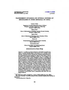
then we can see that 𝑅0 = 𝑅1 + 𝑅2 . Remark 2. We should note from (11) that the use both of vaccine and treatment control to both reduce the value of 𝑅0 , and at the same time effects of both intervention strategies on 𝑅0 are not simply the addition of two independent effects, rather they multiply together in order to improve the overall effects of population level independently (Figure 2). Consider the following: (ii) endemic equilibria, 𝐸∗∗ = (𝑆∗ , 𝐸∗ , 𝐼∗ , 𝐶∗ ), which has four different cases.
Computational and Mathematical Methods in Medicine
5 𝐶2∗ = (𝜆 1 𝜆 2 𝑝3 (] + 𝜆 4 − ]𝑝2 ) 𝑆2∗ (𝑅0 − 1))
6
× ( (] + 𝜆 3 − 𝑝1 ] + 𝑢2 )
Reproduction number
5 4
× [(] + 𝜆 4 − ]𝑝2 ) (] + 𝜆 2 + 𝜆 1 ) + 𝜆 1 𝜆 2 ]
3
+𝜆 1 𝜆 2 𝑝3 (]𝑝1 − ]𝑝2 + 𝜆 4 ) ) .
−1
(14)
2
(c) With vaccine, no treatment control (𝑢1 ≠ 0, 𝑢2 = 0), 𝐸3∗∗ = (𝑆3∗ , 𝐸3∗ , 𝐼3∗ , 𝐶3∗ ), where
1 0
0.1
0
0.2
0.3
0.4 0.5 0.6 Control (u1 , u2 )
u1 = 0, u2 = 0 u1 = 0, u2 = 1
0.7
0.8
0.9
1
u1 = 1, u2 = 0 u1 = 1, u2 = 1
Figure 2: Variation of different reproduction numbers by using of two control variables (vaccination and treatment). Figure 2 illustrates the impact of application of two controls (vaccination and treatment) on different basic reproduction numbers. 𝑅0 = 3.9810, when there is no vaccination and treatment (𝑢1 = 0; 𝑢2 = 0). The figure shows that application of vaccination reduces 𝑅0 more rapidly than treatment, though mixed intervention strategies always work better to reduce the disease burden.
𝑆3∗ =
(] + 𝜆 1 ) (] + 𝜆 2 ) (] + 𝜆 3 − 𝑝1 ]) , 𝜌𝜆 1 (] + 𝜆 3 + 𝜃𝜆 2 𝑝3 − 𝑝1 ])
𝐸3∗ =
𝜃𝜌 (] + 𝜆 2 ) 𝐶3∗ 𝑆3∗ , (] + 𝜆 1 ) (] + 𝜆 2 ) − 𝜌𝜆 1 𝑆3∗
𝐼3∗ =
𝜃𝜌𝜆 1 𝐶3∗ 𝑆3∗ , (] + 𝜆 1 ) (] + 𝜆 2 ) − 𝜌𝜆 1 𝑆3∗
(15)
𝐶3∗ = (𝜆 1 𝜆 2 𝑝3 (] + 𝜆 4 − ]𝑝2 + 𝑢1 ) 𝑆3∗ (𝑅0 − 1)) × ( (] + 𝜆 3 − 𝑝1 ]) × [(] + 𝜆 4 − ]𝑝2 ) (] + 𝜆 2 + 𝜆 1 ) + 𝜆 1 𝜆 2 ]
(a) No vaccine, no treatment control (𝑢1 = 0, 𝑢2 = 0), 𝐸1∗∗ = (𝑆1∗ , 𝐸1∗ , 𝐼1∗ , 𝐶1∗ ), where (] + 𝜆 1 ) (] + 𝜆 2 ) (] + 𝜆 3 − 𝑝1 ]) , 𝑆1∗ = 𝜌𝜆 1 (] + 𝜆 3 + 𝜃𝜆 2 𝑝3 − 𝑝1 ]) 𝐸1∗ = 𝐼1∗ =
𝜆 2 ) 𝐶1∗ 𝑆1∗
𝜃𝜌 (] + , (] + 𝜆 1 ) (] + 𝜆 2 ) − 𝜌𝜆 1 𝑆1∗ 𝜃𝜌𝜆 1 𝐶1∗ 𝑆1∗ , (] + 𝜆 1 ) (] + 𝜆 2 ) − 𝜌𝜆 1 𝑆1∗
(13)
𝐶1∗ = (𝜆 1 𝜆 2 𝑝3 (] + 𝜆 4 − ]𝑝2 ) 𝑆1∗ (𝑅0 − 1))
−1
+𝜆 1 𝜆 2 𝑝3 (]𝑝1 − ]𝑝2 + 𝜆 4 ) ) . (d) With vaccine, with treatment control (𝑢1 ≠ 0, 𝑢2 ≠ 0), 𝐸4∗∗ = (𝑆4∗ , 𝐸4∗ , 𝐼4∗ , 𝐶4∗ ), where 𝑆4∗ =
(] + 𝜆 1 ) (] + 𝜆 2 ) (] + 𝜆 3 − 𝑝1 ] + 𝑢2 ) , 𝜌𝜆 1 (] + 𝜆 3 + 𝜃𝜆 2 𝑝3 − 𝑝1 ] + 𝑢2 )
𝐸4∗ =
𝜃𝛽 (] + 𝜆 2 ) 𝐶4∗ 𝑆4∗ , (] + 𝜆 1 ) (] + 𝜆 2 ) − 𝜌𝜆 1 𝑆4∗
𝐼4∗ =
𝜃𝜌𝜆 1 𝐶4∗ 𝑆4∗ , (] + 𝜆 1 ) (] + 𝜆 2 ) − 𝜌𝜆 1 𝑆4∗
𝐶4∗
× ( (] + 𝜆 3 − 𝑝1 ]) × [(] + 𝜆 4 − ]𝑝2 ) (] + 𝜆 2 + 𝜆 1 ) + 𝜆 1 𝜆 2 ] −1
+𝜆 1 𝜆 2 𝑝3 (]𝑝1 − ]𝑝2 + 𝜆 4 ) ) .
= (𝜆 1 𝜆 2 𝑝3 (] + 𝜆 4 − ]𝑝2 +
𝑢1 ) 𝑆4∗
(16) (𝑅0 − 1))
× ( (] + 𝜆 3 − 𝑝1 ] + 𝑢2 ) × [(] + 𝜆 4 − ]𝑝2 ) (] + 𝜆 2 + 𝜆 1 ) + 𝜆 1 𝜆 2 ] −1
+𝜆 1 𝜆 2 𝑝3 (]𝑝1 − ]𝑝2 + 𝜆 4 ) ) . (b) No vaccine, with treatment control (𝑢1 = 0, 𝑢2 ≠ 0), 𝐸2∗∗ = (𝑆2∗ , 𝐸2∗ , 𝐼2∗ , 𝐶2∗ ), where 𝑆2∗ = 𝐸2∗
(] + 𝜆 1 ) (] + 𝜆 2 ) (] + 𝜆 3 − 𝑝1 ] + 𝑢2 ) , 𝜌𝜆 1 (] + 𝜆 3 + 𝜃𝜆 2 𝑝3 − 𝑝1 ] + 𝑢2 )
𝜃𝜌 (] + 𝜆 2 ) 𝐶2∗ 𝑆2∗ = , (] + 𝜆 1 ) (] + 𝜆 2 ) − 𝜌𝜆 1 𝑆2∗
𝐼2∗ =
𝜃𝜌𝜆 1 𝐶2∗ 𝑆2∗ , (] + 𝜆 1 ) (] + 𝜆 2 ) − 𝜌𝜆 1 𝑆2∗
Clearly 𝐸∗∗ is feasible if 𝐶∗ > 0, that is, if 𝑅0 > 1. Also for 𝑅0 = 1, the endemic equilibrium reduces to the disease-free equilibrium and for 𝑅0 < 1 it becomes infeasible. Hence we may state the following theorem. Theorem 3. (i) If 𝑅0 < 1, then the system (2) has only one equilibrium, which is disease-free. (ii) If 𝑅0 > 1, then the system (2) has two equilibria: one is disease-free and the other is endemic equilibrium. (iii) If 𝑅0 = 1, then the endemic equilibrium reduces to the disease-free equilibrium.
6
Computational and Mathematical Methods in Medicine
3.2. Stability Analysis. In this section, we will discuss the stability of different equilibria. Firstly, we analyse the local stability of the disease-free equilibrium.
Theorem 4. If 𝑅0 < 1, then the disease-free equilibrium is locally asymptotically stable. Proof. The Jacobian matrix of system (2) at the disease-free equilibrium is
− (] + 𝜆 4 − ]𝑝2 + 𝑢1 ) − (𝜆 4 − ]𝑝2 ) − (𝜌𝑆0 + 𝜆 4 − ]𝑝2 ) − (]𝑝1 + 𝜆 4 − ]𝑝2 + 𝜃𝜌𝑆0 ) ] [ 0 − (] + 𝜆 1 ) 𝜌𝑆0 𝜃𝜌𝑆0 ] [ J0 = [ ]. ] [ 0 𝜆1 − (] + 𝜆 2 ) 0 ]𝑝1 − ] − 𝜆 3 − 𝑢2 0 0 𝑝3 𝜆 2 ] [
The characteristic polynomial of 𝐽0 given by 𝑃 (𝜆) = (𝜆 + 𝑙0 ) (𝜆3 + 𝑙1 𝜆2 + 𝑙2 𝜆 + 𝑙3 ) ,
(17)
(a) 𝑙0 , 𝑙1 , 𝑙2 , 𝑙3 > 0; (18)
(b) 𝑙1 𝑙2 − 𝑙3 > 0.
𝑙1 = 3] + 𝜆 1 + 𝜆 2 + 𝜆 3 + 𝑢2 − ]𝑝1 ,
It is easy to see that 𝑙0 , 𝑙1 > 0 and 𝑙2 , 𝑙3 , 𝑙1 𝑙2 − 𝑙3 > 0 if 𝑅0 < 1. It follows from the Routh-Hurwitz criterion that the eigenvalues have negative real parts if 𝑅0 < 1. Hence, the disease-free equilibrium of model (2) is locally asymptotically stable if 𝑅0 < 1 and unstable if 𝑅0 > 1.
𝑙2 = (] + 𝜆 2 ) (] + 𝜆 3 + 𝑢2 − ]𝑝1 )
To discuss the properties of the endemic equilibrium point
where 𝑙0 = ] + 𝑢1 + 𝜆 4 − ]𝑝2 ,
+ (] + 𝜆 1 ) (2] + 𝜆 2 + 𝜆 3 + 𝑢2 − ]𝑝1 ) − 𝜆 1 𝜌𝑆0 ,
(19)
Theorem 5. The endemic equilibrium point is locally asymptotically stable if 𝑅0 > 1.
𝑙3 = (] + 𝜆 1 ) (] + 𝜆 2 ) (] + 𝜆 3 + 𝑢2 − ]𝑝1 ) − 𝜆 1 𝜌𝑆0 (] + 𝜆 3 + 𝑢2 + 𝜃𝑝3 𝜆 2 − ]𝑝1 ) .
Proof. We use Routh-Hurwitz criterion to establish the local stability of the endemic equilibrium. The Jacobian matrix of system (2) at endemic equilibrium is
We need to verify the following two conditions:
− (] + 𝜆 4 − ]𝑝2 + 𝑢1 + 𝜌𝐼∗ ) − (𝜆 4 − ]𝑝2 ) − (𝜌𝑆∗ + 𝜆 4 − ]𝑝2 ) − (]𝑝1 + 𝜆 4 − ]𝑝2 + 𝜌𝜃𝑆∗ ) ] [ 𝜌𝐼∗ + 𝜌𝜃𝐶∗ − (] + 𝜆 1 ) 𝜌𝑆∗ 𝜌𝜃𝑆∗ ]. J∗ = [ ] [ 0 𝜆1 − (] + 𝜆 2 ) 0 𝜆 ]𝑝 − ] − 𝜆 − 𝑢 0 0 𝑝 3 2 1 3 2 ] [ Then the characteristic equation at 𝐸∗∗ is 𝜆4 + 𝑓1 𝜆3 + 𝑓2 𝜆2 + 𝑓3 𝜆 + 𝑓4 = 0, where 𝑓1 = 𝑎1 + 𝑏2 + 𝑐3 + 𝑑4 , 𝑓2 = 𝑎1 𝑎3 + 𝑎1 𝑑4 + 𝑎1 𝑏2 + 𝑐3 𝑑4 + 𝑏2 𝑐3 + 𝑏2 𝑑4 − 𝑏3 𝑐2 − 𝑏1 𝑎2 , 𝑓3 = 𝑎1 𝑐3 𝑑4 + 𝑎1 𝑏2 𝑐3 + 𝑎1 𝑏2 𝑑4 + 𝑏2 𝑐3 𝑑4 + 𝑏4 𝑐2 𝑑3 + 𝑏1 𝑐2 𝑎3 − 𝑎1 𝑏3 𝑐2 − 𝑏3 𝑐2 𝑑4 − 𝑏1 𝑎2 𝑐3 − 𝑏1 𝑎2 𝑑4 , 𝑓4 = 𝑎1 𝑏2 𝑐3 𝑑4 + 𝑎1 𝑏4 𝑐2 𝑑3 + 𝑏1 𝑐2 𝑎3 𝑑4 − 𝑎1 𝑏3 𝑐2 𝑑4
𝑎4 = − (]𝑝1 + 𝜆 4 − ]𝑝2 + 𝜌𝜃𝑆∗ ) , 𝑏2 = − (] + 𝜆 1 ) , 𝑏4 = 𝜌𝜃𝑆∗ , 𝑐2 = 𝜆 1 ,
𝑏1 = 𝜌𝐼∗ + 𝜌𝜃𝐶∗ ,
𝑏3 = 𝜌𝑆∗ ,
𝑐1 = 0, 𝑐3 = − (] + 𝜆 2 ) ,
𝑐4 = 0,
𝑑1 = 0,
𝑑2 = 0,
𝑑3 = 𝑝3 𝜆 2 ,
𝑑4 = ]𝑝1 − ] − 𝜆 3 − 𝑢2 .
− 𝑏1 𝑎2 𝑐3 𝑑4 − 𝑏1 𝑎4 𝑐2 𝑑3 ,
(22)
(21) We need to verify the following three conditions: where
(a) 𝑓1 , 𝑓2 , 𝑓3 , 𝑓4 > 0;
𝑎1 = − (] + 𝜆 4 − ]𝑝2 + 𝑢1 + 𝜌𝐼∗ ) , 𝑎2 = − (𝜆 4 − ]𝑝2 ) ,
(b) 𝑓1 𝑓2 − 𝑓3 > 0; ∗
𝑎3 = − (𝜌𝑆 + 𝜆 4 − ]𝑝2 ) ,
(20)
(c) 𝑓3 (𝑓1 𝑓2 − 𝑓3 ) − 𝑓12 𝑓4 > 0.
Computational and Mathematical Methods in Medicine
7 Our object is to find (𝑢1∗ , 𝑢2∗ ) such that
It is easy to see that conditions (a) and (b) are satisfied. After computations, we can prove that 𝑓3 (𝑓1 𝑓2 − 𝑓3 ) − 𝑓12 𝑓4 > 0 is also valid. The Routh-Hurwitz criterion and those inequalities in (a)–(c) imply that the characteristic equation at 𝐸∗∗ has only roots with negative real part, which certifies the local stability of 𝐸∗∗ .
𝐽 (𝑢1∗ , 𝑢2∗ ) = min 𝐽 (𝑢1 , 𝑢2 ) , where 𝑢1 (𝑡) , 𝑢2 (𝑡) ∈ Γ
4. Optimal Control with Two Objectives
= {𝑢 (𝑡) | 0 ≤ 𝑢 (𝑡) ≤ 𝑢max (𝑡) ≤ 1, 0 ≤ 𝑡 ≤ 𝑇,
One of the early reasons for studying hepatitis B virus (HBV) infection is to improve the control variables and finally to put down the infection of the population. Optimal control is a useful mathematical tool that can be used to make decisions in this case. In the previous sections we have analyzed the model with two control variables, one is treatment and the other is vaccination and we consider their constant controls throughout the analysis. But in fact these control variables should be time dependent. In this section we consider the vaccination and treatment as time-dependent controls in a compact interval of time duration. Our goals here are to put down infection from the population by increasing the recovered individuals and reducing susceptible, exposed, infected, and carrier individuals in a population and to minimize the costs required to control the hepatitis B virus (HBV) infection by using vaccination and treatment. First of all, we construct the objective functional to be optimized as follows:
Here 𝐴 𝑖 , for 𝑖 = 1, . . . , 4 are positive constants that are represented to keep a balance in the size of 𝑆(𝑡), 𝐸(𝑡), 𝐼(𝑡), and 𝐶(𝑡), respectively; 𝐵1 and 𝐵2 , respectively, are the weights corresponding to the controls 𝑢1 and 𝑢2 . 𝑢max is the maximum attainable value for controls (𝑢1 max and 𝑢2 max ); 𝑢1 max and 𝑢2 max will depend on the amount of resources available to implement each of the control measures [26]. The 𝐵1 and 𝐵2 will depend on the relative importance of each of the control measures in mitigating the spread of the disease as well as the cost (human effort, material resources, etc.) of implementing each of the control measures per unit time [26]. Thus, the terms 𝐵1 𝑢12 and 𝐵2 𝑢22 describe the costs associated with vaccination and treatment, respectively. The square of the control variables is taken here to remove the severity of the side effects and overdoses of vaccination and treatment [27].
𝑇
4.1. Optimal Control Solution. For existence of the solution, we consider the control system (24) with initial condition
(23)
1 + (𝐵1 𝑢12 (𝑡) + 𝐵2 𝑢22 (𝑡))] 𝑑𝑡 2 subject to 𝑆 ̇ (𝑡) = ] − ]𝑝1 𝐶 − 𝜌 (𝐼 + 𝜃𝐶) 𝑆 − ]𝑆 − 𝑢1 𝑆
[ [ [ F (x) = [ [ [ [
𝐼 (0) = 𝐼0 ,
𝐶 (0) = 𝐶0 ;
−] − 𝑢1 − 𝜆 4 + ]𝑝2 −𝜆 4 + ]𝑝2 −𝜆 4 + ]𝑝2
−𝜆 4 + ]𝑝2
0
−] − 𝜆 1
0
0
0
𝜆1
−] − 𝜆 2
0
0
0
𝑝3 𝜆 2
] + 𝜌 (𝐼 + 𝜃𝐶) 𝑆 + 𝜆 4 − ]𝑝2 0
] ] ] ]. ] ]
0
]
𝜌 (𝐼 + 𝜃𝐶) 𝑆
(27)
(28)
where 𝑥(𝑡) = (𝑆(𝑡), 𝐸(𝑡), 𝐼(𝑡), 𝐶(𝑡)) is the vector of the state variables and A and F(x) are defined as follows:
𝐶̇ (𝑡) = ]𝑝1 𝐶 + 𝑝3 𝜆 2 𝐼 − (] + 𝜆 3 ) 𝐶 − 𝑢2 𝐶.
[
𝐸 (0) = 𝐸0 ,
𝑑𝑥 (𝑡) = 𝐴𝑥 + 𝐹 (𝑥) , 𝑑𝑡
(24)
𝐼 ̇ (𝑡) = 𝜆 1 𝐸 − (] + 𝜆 2 ) 𝐼,
[ [ [ A= [ [ [ [
𝑆 (0) = 𝑆0 ,
then, we rewrite (2) in the following form:
+ (𝜆 4 − ]𝑝2 ) (1 − 𝑆 − 𝐸 − 𝐼 − 𝐶) , 𝐸̇ (𝑡) = 𝜌 (𝐼 + 𝜃𝐶) 𝑆 − (] + 𝜆 1 ) 𝐸,
(26)
𝑢 (𝑡) is Labesgue measurable} .
𝐽 = ∫ [𝐴 1 𝑆 (𝑡) + 𝐴 2 𝐸 (𝑡) + 𝐴 3 𝐼 (𝑡) + 𝐴 4 𝐶 (𝑡) 0
(25)
] ] ] ], ] ] ]
]𝑝1 − ] − 𝜆 3 − 𝑢2 ]
(29)
8
Computational and Mathematical Methods in Medicine where 𝛼𝑖 (𝑡) for 𝑖 = 1, 2, 3, 4 are the adjoint variables and can be determined by solving the following system of differential equations:
We set
𝐺 (𝑥) = 𝐴𝑥 + 𝐹 (𝑥) .
(30)
𝛼̇1 (𝑡) = −
𝜕𝐻 𝜕𝑆
= − [𝐴 1 + 𝛼1 ((]𝑝2 − 𝜆 4 ) − 𝜌 (𝐼 + 𝜃𝐶) − 𝑢1 − ]) +𝛼2 𝜌 (𝐼 + 𝜃𝐶)] ,
The second term on the right-hand side of (30) satisfies
𝐹 (𝑥1 ) − 𝐹 (𝑥2 ) (31) ≤ 𝑀 (𝑆1 − 𝑆2 + 𝐸1 − 𝐸2 + 𝐼1 − 𝐼2 + 𝐶1 − 𝐶2 ) ,
where the positive constant 𝑀 is independent of the state variables 𝑥 and 𝑀 ≤ 1. Also, we get
𝐺 (𝑥1 ) − 𝐺 (𝑥2 ) ≤ 𝐿 𝑥1 − 𝑥2 ,
𝛼̇2 (𝑡) = −
= − [𝐴 2 + 𝛼1 (]𝑝2 − 𝜆 4 ) + 𝛼2 (−] − 𝜆 1 ) + 𝛼3 𝜆 1 ] , 𝛼̇3 (𝑡) = −
𝜕𝐻 𝜕𝐼
= − [𝐴 3 + 𝛼1 ((]𝑝2 − 𝜆 4 ) − 𝜌𝑆) + 𝛼2 𝜌𝑆 +𝛼3 (−] − 𝜆 2 ) + 𝛼4 𝑝3 𝜆 2 ] , 𝛼̇4 (𝑡) = −
(32)
𝜕𝐻 𝜕𝐸
𝜕𝐻 𝜕𝐶
= − [𝐴 4 + 𝛼1 (]𝑝2 − 𝜆 4 − ]𝑝1 − 𝜌𝜃𝑆) +𝛼2 𝜌𝜃𝑆 + 𝛼4 (]𝑝1 − ] + 𝜆 3 + 𝑢2 )] ,
where 𝐿 = max{𝑀, ‖𝐴‖} < ∞. Therefore, it follows that the function 𝐺 is uniformly Lipschitz continuous. From the definition of the controls 𝑢1 (𝑡) and 𝑢2 (𝑡) and the restrictions on the nonnegativeness of the state variables we see that a solution of the system (28) exists [24, 28, 29].
4.2. The Lagrangian and Hamiltonian for the Control Problem. In order to find an optimal solution pair, first we should find the Lagrangian and Hamiltonian for the optimal control problem (24). In fact, the Lagrangian of problem is given by
(35) satisfying the transversality conditions and optimality conditions: 𝛼1 (𝑇) = 𝛼2 (𝑇) = 𝛼3 (𝑇) = 𝛼4 (𝑇) = 0, 𝜕𝐻 = 𝐵1 𝑢1 − 𝛼1 𝑆 = 0, 𝜕𝑢1
(36)
𝜕𝐻 = 𝐵2 𝑢2 − 𝛼4 𝐶 = 0. 𝜕𝑢2 We now state and prove the following theorem. Theorem 6. There is an optimal control (𝑢1∗ , 𝑢2∗ ) such that
𝐿 (𝑆, 𝐸, 𝐼, 𝐶, 𝑢1 , 𝑢2 ) = 𝐴 1 𝑆 (𝑡) + 𝐴 2 𝐸 (𝑡) + 𝐴 3 𝐼 (𝑡) + 𝐴 4 𝐶 (𝑡) +
1 (𝐵 𝑢2 (𝑡) + 𝐵2 𝑢22 (𝑡)) . 2 1 1 (33)
We are looking for the minimal value of the Lagrangian. To accomplish this, we define Hamiltonian 𝐻 for the control problem as follows:
𝐽 (𝑆, 𝐸, 𝐼, 𝑆, 𝑢1∗ , 𝑢2∗ ) = min 𝐽 (𝑆, 𝐸, 𝐼, 𝑆, 𝑢1 , 𝑢2 )
(37)
subject to the system of differential equation (24). Proof. Here both the control and state variables are nonnegative values. In this minimized problem, the necessary convexity of the objective functional in 𝑢1 and 𝑢2 are satisfied. The set of all control variables 𝑢1 (𝑡), 𝑢2 (𝑡) is also convex and closed by definition. The optimal system is bounded which determines the compactness needed for the existence of the optimal control. In addition, the integrand in the functional 𝑇
∫ [𝐴 1 𝑆 (𝑡) + 𝐴 2 𝐸 (𝑡) + 𝐴 3 𝐼 (𝑡) + 𝐴 4 𝐶 (𝑡) 0
𝐻 (𝑆, 𝐸, 𝐼, 𝐶, 𝑢1 , 𝑢2 , 𝛼1 , 𝛼2 , 𝛼3 , 𝛼4 ) = 𝐿 + 𝛼1 (𝑡)
𝑑𝑆 𝑑𝐸 𝑑𝐼 𝑑𝐶 + 𝛼2 (𝑡) + 𝛼3 (𝑡) + 𝛼4 (𝑡) , 𝑑𝑡 𝑑𝑡 𝑑𝑡 𝑑𝑡 (34)
1 + (𝐵1 𝑢12 (𝑡) + 𝐵2 𝑢22 (𝑡))] 𝑑𝑡 2
(38)
is convex on the control set. Hence the theorem (the proof is complete).
Computational and Mathematical Methods in Medicine
9
4.3. Necessary and Sufficient Conditions for Optimal Controls. Applying Pontryagin’s maximum principle [30] on the constructed Hamiltonian 𝐻, and the theorem (24), we obtain the optimal steady-state solution and corresponding control as follows: If taking 𝑋 = (𝑆, 𝐸, 𝐼, 𝐶) and 𝑈 = (𝑢1 , 𝑢2 ), then (𝑋∗ , 𝑈∗ ) is an optimal solution of an optimal control problem; then we now state the following theorem. Theorem 7. The optimal control pair (𝑢1∗ , 𝑢2∗ ) which minimizes J over the region Γ is given by 𝑢1 (𝑡) , 1)} , 𝑢1∗ = max {0, min (̃ [0,𝑇]
𝑢2∗ = max {0, min (̃ 𝑢2 (𝑡) , 1)} ,
(39)
[0,𝑇]
where 𝑢̃1 = 𝛼̃1 𝑆/𝐵1 and 𝑢̃2 = 𝛼̃4 𝐶/𝐵2 and let {̃ 𝛼1 , 𝛼̃2 , 𝛼̃3 , 𝛼̃4 } be the solution of system (35). Proof. With the help of the optimality conditions, we have 𝛼̃ 𝑆 𝜕𝐻 = 𝐵1 𝑢1 − 𝛼1 𝑆 = 0 ⇒ 𝑢1 = 1 = (̃ 𝑢1 ) , 𝜕𝑢1 𝐵1 𝛼̃ 𝐶 𝜕𝐻 = 𝐵2 𝑢2 − 𝛼4 𝐶 = 0 ⇒ 𝑢2 = 4 = (̃ 𝑢2 ) . 𝜕𝑢2 𝐵2
(40)
Using the property of the control space Γ, the two controls which are bounded with upper and lower bounds are, respectively, 1 and 0; that is, 0 { { 𝑢1∗ = {𝑢̃1 { {1
if 𝑢̃1 ≤ 0 if 0 < 𝑢̃1 < 1 if 𝑢̃1 ≥ 1.
(41)
This can be rewritten in compact notation 𝑢1∗ = max {0, min (̃ 𝑢1 (𝑡) , 1)} , [0,𝑇]
(42)
and similarly 𝑢2∗
0 { { = {𝑢̃2 { {1
if 𝑢̃2 ≤ 0 if 0 < 𝑢̃2 < 1 if 𝑢̃2 ≥ 1.
(43)
This can be rewritten in compact notation 𝑢2∗ = max {0, min (̃ 𝑢2 (𝑡) , 1)} . [0,𝑇]
(44)
Hence for these pair of controls (𝑢1∗ , 𝑢2∗ ) we get the optimum value of the functional 𝐽 given by (24).
5. Numerical Examples Numerical solutions to the optimality system (24) are discussed in this section. We make several interesting observation by numerically simulating (2) in the range of parameter values. We consider the parameter set
Δ = {], 𝜌, 𝜃, 𝜆 1 , 𝜆 2 , 𝜆 3 , 𝜆 4 , 𝑝1 , 𝑝2 , 𝑝3 , 𝐴 1 , 𝐴 2 , 𝐴 3 , 𝐴 4 , 𝐵1 , 𝐵2 }; some of the parameters are taken from the published articles and some are assumed with feasible values. Moreover, the time interval for which the optimal control is applied is taken as 70 years; also consider Ψ = {𝑆0 , 𝐸0 , 𝐼0 , 𝐶0 } as initial condition for simulation of the model. The main parameter values are listed in Table 1. We compare the results having no controls, only vaccination control, only treatment control, and both vaccination and treatment controls. With the parameter values in Table 1, the system asymptotically approaches towards the equilibrium 𝐸1∗∗ (0.0858, 0.3327, 0.4003, 0.5349), where the basic reproduction ratio 𝑅0 = 3.9810 (Figure 2). For the parameters set the system (2) has two feasible equilibria; one is disease free and the other is endemic, and the endemic equilibrium is locally asymptotically stable. The effect of two control measures on disease dynamics may be understood well if we consider Figure 2. It explains how control reproduction ratio 𝑅0 evolves with different rates of 𝑢1 and 𝑢2 . It is seen that both vaccination and treatment reduce the value of 𝑅0 effectively. But an integrated control works better than either of the control measures. In this section, we use an iterative method to obtain results for an optimal control problem of the proposed model (24). We use Runge-Kutta’s fourth-order procedure [23] here to solve the optimality system consisting of eight ordinary differential equations having four state equations and four adjoint equations and boundary conditions. Because state equations have initial conditions and adjoint equations have conditions at the final time, an iterative program was created to numerically simulate solutions. Given an initial guess for the controls, to compute the optimal state values, the program solves (24) with initial conditions (27) forward in time interval [0, 70] using a Runge Kutta method of the fourth order. Resulting state values are placed in adjoint equations (35). These adjoint equations with given final conditions are then solved backwards in time. Again, a fourth order Runge Kutta method is employed. Both state and adjoint values are used to update the control using the characterization (39) and the entire process repeats itself. This iterative process terminates when current state, adjoint, and control values are sufficiently close to successive values. Then we use the backward Runge-Kutta fourth-order procedure to solve the adjoint variables in the same time interval with the help of the solution of the state variables transversality conditions. We have plotted susceptible, exposed, acute infection individuals, and carriers individuals with and without control by considering values of parameters. We simulate the system at different values of rate of 𝑢1 and 𝑢2 . From Figures 3, 4, and 5, we see that after 20 years the number of susceptible population decreases than when there is no control. In this case most of this population tends to the infected class. Again when only treatment control is applied, then the number of susceptible population is not much different than the population in the case having no control. But the susceptible population differs much from these two strategies if we apply the strategies of only vaccination control and both vaccination and treatment controls. At a high rate of vaccination, the sensitive population density is reduced
10
Computational and Mathematical Methods in Medicine Table 1: Parameter values used in numerical simulations.
Parameter ] 𝜌 𝜃 𝜆1 𝜆2 𝜆3 𝜆4 𝑃1 𝑃2 𝑃3 𝐴1 𝐴2 𝐴3 𝐴4 𝐵1 𝐵2 𝑆0 𝐸0 𝐼0 𝐶0
Description Birth (and death) rate Transmission rate Infectiousness of carriers relative to acute infections Rate of moving from exposed to acute Rate at which individuals leave the acute infection class Rate of moving from carrier to recovery Loss of recovery rate Probability of infected newborns Probability of immune newborns Proportion of acute infection individuals becoming carriers Weight factor for susceptible individuals Weight factor for exposed individuals Weight factor for infected individuals Weight factor for carrier individuals Weight factor for the controls 𝑢1 Weight factor for the controls 𝑢2 Susceptible individuals Exposed individuals Acute infection individuals Chronic HBV carriers
10−1
10−2
10−1 10−2 10−3 10−4
10−3
10−4
Reference [17, 18] [17] [17] [16] [16] [16] [17] [19] [19] [17] [31] [31] [31] [31] [31] [31] [4] [4] [4] [4]
100 Susceptible population
Susceptible population
100
Values range 0.0121 0.8–20.49 0-1 6 per year 4 per year 0.025 per year 0.03–0.06 0.11 0.1 0.05–0.9 0.091 0.01 0.04 0.05 1.5 2.7 0.493 0.0035 0.0035 0.007
0
10
NV-NT NV-T
20
30 40 Time (year)
50
60
70
V-NT V-T
Figure 3: The plot shows the changes in sensitive populations (without) vaccination and (without) treatment.
to a very low level initially and then it takes longer time to restore the steady-state value. From Figures 6, 7, and 8, we see that the number of exposed population increase than when there is no control. In this case, most of this population tends to the acute infected class. Again when only treatment control is applied, then the number of exposed population is not much different
0
10
20
u1 = 0, u2 = 0 u1 = 0.365, u2 = 0 u1 = 0.45, u2 = 0
30 40 Time (year)
50
60
70
u1 = 0.73, u2 = 0 u1 = 0.9, u2 = 0 u1 = 0.9, u2 = 0.9
Figure 4: The plot shows the sensitivity of sensitive populations for different values of control 𝑢1 .
than the population in the case having no control. But the exposed population differs much from these two strategies if we apply the strategies of only vaccination control and both vaccination and treatment controls. From Figures 9, 10, and 11, we see that the number of acute infected population increases than when there is no control. In this case most of this population tends to the carrier class. Again when only treatment control is applied, then the number of acute infected population is not much different than the population in the case having no control. But the acute infected population differs much from these two
Computational and Mathematical Methods in Medicine
11 100
10−1 10−1 10−2
Exposed population
Susceptible population
100
10−3 10−4
0
10
20
u1 = 0, u2 = 0 u1 = 0, u2 = 0.365 u1 = 0, u2 = 0.45
30 40 Time (year)
50
60
70
10−2
10−3
u1 = 0, u2 = 0.73 u1 = 0, u2 = 0.9 u1 = 0.9, u2 = 0.9
10−4
0
Figure 5: The plot shows the sensitivity of sensitive populations for different values of control 𝑢2 .
100
30 40 Time (year)
50
60
70
u1 = 0.73, u2 = 0 u1 = 0.9, u2 = 0 u1 = 0.9, u2 = 0.9
Figure 7: The plot shows the sensitivity of exposed populations for different values of control 𝑢1 . 100
10−2
10−1 Exposed population
Exposed population
20
u1 = 0, u2 = 0 u1 = 0.3635, u2 = 0 u1 = 0.45, u2 = 0
10−1
10−3
10−4
10
0
10
NV-NT NV-T
20
30 40 Time (year)
50
60
70
V-NT V-T
Figure 6: The plot shows the changes in exposed populations (without) vaccination and (without) treatment.
10−2
10−3
10−4
0
10
20
u1 = 0, u2 = 0 u1 = 0, u2 = 0.365 u1 = 0, u2 = 0.45
strategies if we apply the strategies of only vaccination control and both vaccination and treatment controls. Again from Figures 12, 13, and 14, we see that the number of carrier population increases than when there is no control. We see that the application of only vaccination control gives better result than the application of no control. Again application of treatment control would give better result than the application of vaccination control since the treatment control is better than the vaccination control while the application of both vaccination and treatment controls give the best result as in this case the number of carrier population would be the least in number.
30 40 Time (year)
50
60
70
u1 = 0, u2 = 0.73 u1 = 0, u2 = 0.9 u1 = 0.9, u2 = 0.9
Figure 8: The plot shows the sensitivity of exposed populations for different values of control 𝑢2 .
Finally, the effect of two control measures on disease dynamics may be understood well if we consider Figures 1– 14, 15, 16, 17, and 18. Since our main purpose is to reduce the number of sensitive, exposed, acute infection, and carrier individuals, therefore numerical simulation results show that optimal combination of vaccination and treatment is the most effective way to control hepatitis B virus infection.
Computational and Mathematical Methods in Medicine 100
100
10−1
10−1
Acute infection population
Acute infection population
12
10−2
10−3
10−4
0
10
20
30 40 Time (year)
50
60
10−2
10−3
10−4
70
0
10
20
30
40
50
60
70
Time (year) V-NT V-T
NV-NT NV-T
Figure 9: The plot shows the changes in acute infection populations (without) vaccination and (without) treatment.
u1 = 0, u2 = 0 u1 = 0, u2 = 0.365 u1 = 0, u2 = 0.45
u1 = 0, u2 = 0.73 u1 = 0, u2 = 0.9 u1 = 0.9, u2 = 0.9
Figure 11: The plot shows the sensitivity of acute infection populations for different values of control 𝑢2 .
100
10−1
10
Carrier population
Acute infection population
100
−2
10−3
10−4
10−1 10−2 10−3 10−4
0
10
20
u1 = 0, u2 = 0 u1 = 0.365, u2 = 0 u1 = 0.45, u2 = 0
30 40 Time (year)
50
60
70
u1 = 0.73, u2 = 0 u1 = 0.9, u2 = 0 u1 = 0.9, u2 = 0.9
Figure 10: The plot shows the sensitivity of acute infection populations for different values of control 𝑢1 .
6. Conclusion and Suggestions In this paper, we propose an S-𝐸-𝐼-𝐶-𝑅 model of hepatitis B virus infection with two controls: vaccination and treatment. First we analyze the dynamic behavior of the system for constant controls. In the constant controls case, we calculate the basic reproduction number and investigate the existence and stability of equilibria. There are two nonnegative equilibria of
0
10
NV-NT NV-T
20
30 40 Time (year)
50
60
70
V-NT V-T
Figure 12: The plot shows the changes in carrier populations (without) vaccination and (without) treatment.
the system, namely, the disease-free and endemic. We see that the disease-free equilibrium which always exists and is locally asymptotically stable if 𝑅0 < 1, and endemic equilibrium which exists and is locally asymptotically stable if 𝑅0 > 1. After investigating the dynamic behavior of the system with constant controls we formulate an optimal control problem if the controls become time dependent and solve it by using Pontryagin’s maximum principle. Different possible combinations of controls are used and their effectiveness is compared by simulation works. Also, from the numerical results it is very clear that a combination of mixed control measures respond better than any other independent control.
Computational and Mathematical Methods in Medicine
13
100
Population (NV-NT)
Carrier population
10
100
−1
10−2
10−2 10−3 10−4
10−3
10−4
10−1
0
10
20
30 40 Time (year)
S E 0
10
20
30 40 Time (year)
50
60
70
60
70
I C
Figure 15: The plot shows the changes in total populations without vaccination and without treatment.
u1 = 0.73, u2 = 0 u1 = 0.9, u2 = 0 u1 = 0.9, u2 = 0.9
u1 = 0, u2 = 0 u1 = 0.365, u2 = 0 u1 = 0.46, u2 = 0
50
100
Population (V-NT)
Figure 13: The plot shows the sensitivity of carrier populations for different values of control 𝑢1 .
100
10−1 10−2 10−3
Carrier population
10−1 10−4
0
10−2
20
30 40 Time (year)
S E
50
60
70
I C
Figure 16: The plot shows the changes in total populations with vaccination and without treatment.
10−3
10−4
10
0
10
20
30
40
50
60
100
70
u1 = 0, u2 = 0 u1 = 0, u2 = 0.365 u1 = 0, u2 = 0.45
u1 = 0, u2 = 0.73 u1 = 0, u2 = 0.9 u1 = 0.9, u2 = 0.9
Figure 14: The plot shows the sensitivity of carrier populations for different values of control 𝑢2 .
There is still a tremendous amount of work needed to be done in this area. Parameters are rarely constant because they depend on environmental conditions. We do not know, however, the detailed relationship between these parameters and environmental conditions. There may be a time lag as a susceptible population may take some time to be infected and also a susceptible population may take some time to immune
Population (NV-T)
Time (year) 10−1 10−2 10−3 10−4
0
10 S E
20
30 40 Time (year)
50
60
70
I C
Figure 17: The plot shows the changes in total populations without vaccination and with treatment.
14
Computational and Mathematical Methods in Medicine
Population (V-T)
100
[11]
10−1
[12]
10−2 10−3 10−4
[13]
0
10
20
S E
30 40 Time (year)
50
60
70
[14] I C
Figure 18: The plot shows the changes in total populations with vaccination and treatment.
after vaccination. We leave all these possible extensions for the future work.
Conflict of Interests
[15] [16]
[17]
[18]
The authors declare that there is no conflict of interests regarding the publication of this paper.
[19]
References
[20]
[1] WHO, Hepatitis B Fact Sheet No. 204, The World Health Organisation, Geneva, Switzerland, 2013, http://www.who.int/ mediacentre/factsheets/fs204/en/. [2] Canadian Centre for Occupational Health and Safety, “Hepatitis B,” http://www.ccohs.ca/oshanswers/diseases/hepatitis b.html. [3] “Healthcare stumbling in RI’s Hepatitis fight,” The Jakarta Post, January 2011. [4] G. F. Medley, N. A. Lindop, W. J. Edmunds, and D. J. Nokes, “Hepatitis-B virus endemicity: heterogeneity, catastrophic dynamics and control,” Nature Medicine, vol. 7, no. 5, pp. 619–624, 2001. [5] J. Mann and M. Roberts, “Modelling the epidemiology of hepatitis B in New Zealand,” Journal of Theoretical Biology, vol. 269, no. 1, pp. 266–272, 2011. [6] “Hepatitis B, (HBV),” http://kidshealth.org/teen/sexual health/ stds/std hepatitis.html. [7] CDC, “Hepatitis B virus: a comprehensive strategy for eliminating transmission in the United States through universal childhood vaccination. Recommendations of the Immunization Practices Advisory Committee (ACIP),” MMWR Recommendations and Reports, vol. 40(RR-13), pp. 1–25, 1991. [8] M. K. Libbus and L. M. Phillips, “Public health management of perinatal hepatitis B virus,” Public Health Nursing, vol. 26, no. 4, pp. 353–361, 2009. [9] F. B. Hollinger and D. T. Lau, “Hepatitis B: the pathway to recovery through treatment,” Gastroenterology Clinics of North America, vol. 35, no. 4, pp. 895–931, 2006. [10] C.-L. Lai and M.-F. Yuen, “The natural history and treatment of chronic hepatitis B: a critical evaluation of standard treatment
[21]
[22]
[23]
[24] [25]
[26]
[27]
[28]
[29]
criteria and end points,” Annals of Internal Medicine, vol. 147, no. 1, pp. 58–61, 2007. R. M. Anderson and R. M. May, Infectious Disease of Humans: Dynamics and Control, Oxford University Press, Oxford, UK, 1991. S. Thornley, C. Bullen, and M. Roberts, “Hepatitis B in a high prevalence New Zealand population: a mathematical model applied to infection control policy,” Journal of Theoretical Biology, vol. 254, no. 3, pp. 599–603, 2008. S.-J. Zhao, Z.-Y. Xu, and Y. Lu, “A mathematical model of hepatitis B virus transmission and its application for vaccination strategy in China,” International Journal of Epidemiology, vol. 29, no. 4, pp. 744–752, 2000. K. Wang, W. Wang, and S. Song, “Dynamics of an HBV model with diffusion and delay,” Journal of Theoretical Biology, vol. 253, no. 1, pp. 36–44, 2008. R. Xu and Z. Ma, “An HBV model with diffusion and time delay,” Journal of Theoretical Biology, vol. 257, no. 3, pp. 499–509, 2009. L. Zou, W. Zhang, and S. Ruan, “Modeling the transmission dynamics and control of hepatitis B virus in China,” Journal of Theoretical Biology, vol. 262, no. 2, pp. 330–338, 2010. J. Pang, J.-A. Cui, and X. Zhou, “Dynamical behavior of a hepatitis B virus transmission model with vaccination,” Journal of Theoretical Biology, vol. 265, no. 4, pp. 572–578, 2010. S. Zhang and Y. Zhou, “The analysis and application of an HBV model,” Applied Mathematical Modelling, vol. 36, no. 3, pp. 1302– 1312, 2012. S. Bhattacharyya and S. Ghosh, “Optimal control of vertically transmitted disease,” Computational and Mathematical Methods in Medicine, vol. 11, no. 4, pp. 369–387, 2010. T. K. Kar and A. Batabyal, “Stability analysis and optimal control of an SIR epidemic model with vaccination,” Biosystems, vol. 104, no. 2-3, pp. 127–135, 2011. T.-K. Kar and S. Jana, “A theoretical study on mathematical modelling of an infectious disease with application of optimal control,” Biosystems, vol. 111, no. 1, pp. 37–50, 2013. M. J. Keeling and P. Rohani, Modeling Infectious Diseases in Humans and Animals, Princeton University Press, Princeton, NJ, USA, 2008. E. Jung, S. Lenhart, and Z. Feng, “Optimal control of treatments in a two-strain tuberculosis model,” Discrete and Continuous Dynamical Systems B, vol. 2, no. 4, pp. 473–482, 2002. G. Birkhoff and G.-C. Rota, Ordinary Differential Equations, John Wiley & Sons, New York, NY, USA, 4th edition, 1989. P. van den Driessche and J. Watmough, “Reproduction numbers and sub-threshold endemic equilibria for compartmental models of disease transmission,” Mathematical Biosciences, vol. 180, pp. 29–48, 2002. T. T. Yusuf and F. Benyah, “Optimal control of vaccination and treatment for an SIR epidemiological model,” World Journal of Modelling and Simulation, vol. 8, no. 3, pp. 194–204, 2008. H.-R. Joshi, S. Lenhart, M. Y. Li, and L. Wang, “Optimal control methods applied to disease models,” in Mathematical Studies on Human Disease Dynamics, vol. 410 of Contemporary Mathematics, pp. 187–207, American Mathematical Society, Providence, RI, USA, 2006. G. Zaman, Y. H. Kang, and I. H. Jung, “Stability analysis and optimal vaccination of an SIR epidemic model,” Biosystems, vol. 93, no. 3, pp. 240–249, 2008. D. Iacoviello and N. Stasiob, “Optimal control for SIRC epidemic outbreak,” Computer Methods and Programs in Biomedicine, vol. 110, no. 3, pp. 333–342, 2013.
Computational and Mathematical Methods in Medicine [30] L. S. Pontryagin, V. G. Boltyanskii, R. V. Gamkrelidze, and E. F. Mishchenko, The Mathematical Theory of Optimal Processes, John Wiley & Sons, New York, NY, USA, 1962. [31] WHO, Hepatitis B Fact Sheet No. 204, The World Health Organisation, Geneva, Switzerland, 2000, http://www.who.int/ mediacentre/factsheets/fs204/en/.
15