Mathematical models of ice stream dynamics and

i

i

i

i

POLITECNICO DI TORINO

SCUOLA INTERPOLITECNICA DI DOTTORATO Doctoral Program in Engineeering for the Natural and Built Environment – 28th cycle

Final Dissertation

Mathematical models of ice stream dynamics and supraglacial drainage

Elisa Mantelli Advisor Prof. C. Camporeale

Program Coordinator Prof. C. Scavia

April 2016

i

i i

i

i

i

i

i

This work is subject to the Creative Commons Licence

i

i i

i

i

i

i

i

Abstract Patterning is a recurrent feature of glacial systems, which characterizes as much subglacial and supraglacial environments as the flow of ice itself. Some examples include bedforms developing at the contact between ice and bed, spatial organization in subglacial and supraglacial drainage networks, the narrow corridors of fast flowing ice known as ice streams that form the arterial drainage system of large ice sheets, and temporal switches between slow and fast flow regimes in glacier and ice stream flow. This thesis focusses on two types of glacial patterns, namely ice streams (Part I) and channelization in supraglacial drainage networks (Part II). Ice flow within ice sheets is far from uniform, with the narrow bands known as ice streams flowing at velocity two order of magnitude larger than the rest of the ice sheet. In the Siple Coast region of West Antarctica ice streams experiance weak topographic confinement, thus suggesting that they may originate spontaneously from an otherwise uniform flow as a fingering instability. Motivated by observations suggesting that the marked contrast in velocity between ice streams and surrounding ice is due to a transition from frozen, thus sticky bed underneath slow flowing regions, to molten, thus well lubricated bed under ice streams, we investigate the role of basal thermal transitions in relation to the onset of ice streams. Our findings in chapter 2 suggest that basal transitions from frozen to molten bed (or vice versa) can undergo an instability potentially leading to the onset of streaming. An asymptotic analysis for short wavelength perturbations shows that, at wavelengths of a few ice thicknesses, such instability is controlled by the interplay between strain heating and heat advection from the region upstream of the transition. We also find that the background structure of the ice sheet is key to pattern formation. In particular, in the case of ice flowing from molten to frozen regions we find an instability at the ice sheet thickness scale or smaller, which is not resolved by most ice sheet models. Observations reveal that ice streams experience significant temporal variability iii

i

i i

i

i

i

i

i

on a variety of time scales, ranging from decadal to multi-millennial ones. As much as spatial patterning, such variability holds implications for the future of ice sheets, sea level change, and the interpretation of geological records. Recent work (Robel et al., 2013) shows that the switch between steady streaming conditions and self-sustained oscillations with multi-millennial periodicity can be understood as a Hopf bifurcation. Little is presently known about shorter scale variability, which however appears more likely to originate from external forcing. In chapter 3 we explore the effects of a specific type of forcing, i.e. stochastically-varying climatic conditions, on the temporal dynamics of ice stream flow. We find that data-based climate fluctuations alter the deterministic dynamics substantially, and are capable of introducing widespread, short-scale oscillations even in ranges of the parametric regime where the deterministic dynamics predict steady streaming. We thus conclude that noise-induced transitions may play a role in the observed temporal dynamics of ice stream flow. In Part II we turn to patterning in drainage networks on the surface of glaciers. Supraglacial drainage networks route meltwater originating on the surface of glaciers towards moulins and crevasses, through which it eventually reaches the base of the ice. Therefore, understanding the physical controls on the structure of the drainage network has implications for how surface melt influences the motion of ice. Here we focus on the physical controls on the formation of evenly spaced channels on the surface of glaciers. In particular, we find that the flow of meltwater on bare ice is capable of carving evenly spaced channels as a result of a morphological instability. We show that in certain conditions the network is shaped solely by the hydrodynamics of meltwater regardless of ice thermal conditions, which justifies widely-observed regular patterns in drainage networks. Finally, comparison of our results with the geometrical feature of supraglacial networks reported in the literature shows good agreement between model’s predictions and observations.

iv

i

i i

i

i

i

i

i

Preface The thesis is composed of three individual studies that address specific aspects of the spatial and temporal dynamics of ice stream flow (Part I), and of spatial organization in supraglacial drainage (Part II). The study on basal thermal transitions in chapters 1 and 2 has been conducted in collaboration with Christian Schoof at the University of British Columbia, in fulfillment to the requirements of the Scuola Interpolitecnica di Dottorato. I presented part of this study at the Fall Meeting of the American Geophysical Union in December 2015 (Mantelli et al., 2015b), and a manuscript is in preparation for a fluid mechanics journal. Marianne Haseloff provided the numerical solution of the boundary layer model. Outputs of these computations are included in the thesis for completeness. A version of chapter 3 is currently under review for the Proceedings of the National Academy of Science of the United States of America. The authors are Elisa Mantelli (lead author), Matteo Bertagni and Luca Ridolfi. I was responsible for conducting the research, interpreting results and composing the manuscript. Matteo Bertagni worked on this project as part of his Master dissertation, and was responsible for the computations including stochastic forcing. Luca Ridolfi provided continuous guidance during all of these stages. A version of part II has been published on Water Resources Research (Mantelli et al., 2015a). I was responsible for conducting the research, interpreting results and composing the manuscript. Carlo Camporeale and Luca Ridolfi provided continuous support during all of these stages.

v

i

i i

i

i

i

i

i

i

i i

i

i

i

i

i

Table of Contents Abstract

iii

Preface

v

Acknowledgements

xi

I

1

Ice Stream Dynamics

3

Introduction 1

2

. . . . . . . . . . .

9 11 13 17 17 18 24 25 28 29 30 33

Stability of Basal Thermal Transitions 2.1 Steady States . . . . . . . . . . . . . . . . . . . . . . . . . . . . . . . . 2.1.1 Multivaluedness of the Flux Law . . . . . . . . . . . . . . . . 2.1.2 A Gap in the Flux Law . . . . . . . . . . . . . . . . . . . . . .

37 38 38 41

Ice flow across basal thermal transitions 1.1 Geometry . . . . . . . . . . . . . . . . . . . . . . . 1.2 A Three-dimensional Ice Sheet Model . . . . . . 1.3 Simplified Model . . . . . . . . . . . . . . . . . . 1.3.1 Non-dimensionalization . . . . . . . . . . 1.3.2 A Conductive Ice Sheet Model . . . . . . 1.4 The Boundary Layer . . . . . . . . . . . . . . . . 1.4.1 Problem Formulation . . . . . . . . . . . 1.4.2 Series Expansion . . . . . . . . . . . . . . 1.4.3 Matching . . . . . . . . . . . . . . . . . . . 1.4.4 Implications for the Large Scale Problem 1.5 Discussion . . . . . . . . . . . . . . . . . . . . . .

. . . . . . . . . . .

. . . . . . . . . . .

. . . . . . . . . . .

. . . . . . . . . . .

. . . . . . . . . . .

. . . . . . . . . . .

. . . . . . . . . . .

. . . . . . . . . . .

. . . . . . . . . . .

. . . . . . . . . . .

vii

i

i i

i

i

i

i

i

. . . . . . . .

42 46 50 54 54 58 63 66

Stochastic Temporal Dynamics of Ice Streams 3.1 Introduction . . . . . . . . . . . . . . . . . . . . . . . . . . . . . . . . 3.2 The model by Robel et al. . . . . . . . . . . . . . . . . . . . . . . . . 3.2.1 Model Statement . . . . . . . . . . . . . . . . . . . . . . . . . 3.2.2 Deterministic Dynamics . . . . . . . . . . . . . . . . . . . . . 3.3 Simulating Climate Variability . . . . . . . . . . . . . . . . . . . . . 3.4 Stochastic Ice Stream Dynamics . . . . . . . . . . . . . . . . . . . . . 3.4.1 The Bifurcation Diagram . . . . . . . . . . . . . . . . . . . . . 3.4.2 Simultaneous Forcing of Surface Temperature and Snow Accumulation . . . . . . . . . . . . . . . . . . . . . . . . . . . . 3.4.3 Probability Density Functions . . . . . . . . . . . . . . . . . . 3.5 Discussion and Conclusions . . . . . . . . . . . . . . . . . . . . . . .

71 71 72 73 75 78 80 81

2.2 2.3

2.4 3

II

2.1.3 Oblique Basal Transitions . . . 2.1.4 Sub-temperate Sliding . . . . . Solution of the Boundary Layer Model Stability . . . . . . . . . . . . . . . . . . 2.3.1 Linearization . . . . . . . . . . 2.3.2 Short Wavelength Asymptotics 2.3.3 The Sensitivities of Vm . . . . . Discussion and Conclusions . . . . . .

. . . . . . . .

. . . . . . . .

. . . . . . . .

. . . . . . . .

. . . . . . . .

. . . . . . . .

. . . . . . . .

. . . . . . . .

. . . . . . . .

. . . . . . . .

. . . . . . . .

. . . . . . . .

. . . . . . . .

. . . . . . . .

. . . . . . . .

. . . . . . . .

Supraglacial Drainage

89 91

Introduction 4

83 85 87

Modelling Supraglacial Channelization 4.1 The Model . . . . . . . . . . . . . . . 4.2 Stability Analysis . . . . . . . . . . . 4.3 Channel Formation . . . . . . . . . . 4.3.1 Processes . . . . . . . . . . . . 4.3.2 Parameter Sensitivity . . . . . 4.4 Wavelength Selection . . . . . . . . . 4.5 Relevance to Field Observations . . 4.6 Discussion and Conclusions . . . . .

. . . . . . . .

. . . . . . . .

. . . . . . . .

. . . . . . . .

. . . . . . . .

. . . . . . . .

. . . . . . . .

. . . . . . . .

. . . . . . . .

. . . . . . . .

. . . . . . . .

. . . . . . . .

. . . . . . . .

. . . . . . . .

. . . . . . . .

. . . . . . . .

. . . . . . . .

. . . . . . . .

95 98 105 107 109 112 115 120 122

A Appendix to Chapter 1 125 A.1 Three-Dimensional Boundary Layer Model . . . . . . . . . . . . . . 125 viii

i

i i

i

i

i

i

i

B Appendix to Chapter 4 B.1 Scaling . . . . . . . . . . . . . . . . . . . . . . . . . . . . B.2 Parameterization of Heat Transfer Between Water and sphere . . . . . . . . . . . . . . . . . . . . . . . . . . . . B.3 Solution of the Linearized Problem . . . . . . . . . . . .

131 . . . . . . . 131 the Atmo. . . . . . . 132 . . . . . . . 132 134

References

ix

i

i i

i

i

i

i

i

i

i i

i

i

i

i

i

Acknowledgements I wish to express my thanks to: My advisor, Carlo Camporeale, without whom this adventure would have not even started, and to Luca Ridolfi for their genuine enthusiasm, open-mindedness and generous scientific support that had never been missing over the last three years. Christian Schoof, who holds responsibility for introducing me to the world of asymptotics and ice sheet modelling, for hospitality at the Glaciology Group of the University of British Columbia, for an exciting ’little intellectual adventure’, and - almost equally important - for an intense canadian climbing season. Valerio Bertoglio, who taught me a while ago to look at the mountains with fresh eyes, and that turning a burning passion into a job is something to strive for. Marianne Haseloff, for sharing highs and lows of graduate school, for endless patience with last minute changes, and still providing all the support I could have hoped for. Alessandra, for warm hospitality in Berkeley and sharing life at any distance since a long while ago, and to Valentina and Kathi for making me feel at home in Vancouver. All the fellow students of the first floor (and appendixes!) at the Department of Environment, Land and Infrastructure Engineering at Politecnico di Torino, for making these years a memorable time. I am particularly grateful to Anna, Riccardo and Andrea G. for patiently listening to my obscure mathematical thoughts whenever needed! Stefano: not many words are needed here, I guess... nothing would have been the same if you had not been with me, soundly, over all of this time. Last, my family, for having always been firm foundation to build on.

xi

i

i i

i

i

i

i

i

Financial support from Politecnico di Torino and the Italian Ministry of Education in the form of a three-year scholarship, from Scuola Interpolitecnica di Dottorato, and from the American Geophysical Union in the form of a travel grant to attend the 2013 Fall Meeting in San Francisco is gratefully acknowledged.

xii

i

i i

i

i

i

i

i

A Stefano

i

i i

i

i

i

i

i

i

i i

i

i

i

i

i

Part I

Ice Stream Dynamics

i

i i

i

i

i

i

i

i

i i

i

i

i

i

i

Introduction Ice streams are intrinsic features of ice sheets. These narrow corridors of fastflowing ice, around 50 km wide and stretching into the interior of an ice sheet for up to 500 km, move at speeds two-to-three orders of magnitude greater than the remainder of the sheet. Ice streams are key to ice sheet dynamics, as their ability to collect most of the discharge reshapes geometry and flow field of the surrounding ice. Their prominent role is to efficiently drain snow falling over the continent to the edge of the ice sheet, where it either melts, or is discharged into the ocean as icebergs. In Antarctica, ice streams cover only 10% of the ice sheet surface but may account for over 80% of the ice transport to the coast (Bamber et al., 2000). Since mass loss from Antarctica takes place mostly in ice shelves (i.e., the floating portions of ice sheets that are maintained by the inflow of continental ice from grounded portions of the ice sheet), predominantly by iceberg calving at the edges or by basal melting due to warm ocean water (e.g., Jenkins & Doake, 1991; Jacobs et al., 1992; Rignot et al., 2013), ice discharge from ice streams appears to be a major contributor to sea level rise.

Spatial Patterning The apparent regularity of the spacing of some ice streams, along with their ability to spontaneously shift location (e.g., Retzlaff & Bentley, 1993; Bindschadler & Vornberger, 1998; Hulbe & Fahnestock, 2007; Catania et al., 2012), are suggestive of an instability of the ice flow leading to spatial patterning. The Siple Coast region of West Antarctica provides a contemporary example (figure 1), with five regularly spaced streams whose position is only weakly constrained by topographic highs (Bennett, 2003). This spatial structure points to a fingering instability, with soft, fast-flowing ice protruding into regions of stiff, slow-flowing ice. In fact adjacent streams, which are underlain by a bed at the melting-point (temperate-based), are intervened by ice ridges that are instead frozen to their bed (cold-based) 3

i

i i

i

i

i

i

i

Figure 1: Antarctic ice streams. Left Panel: surface velocity map of West Antarctica (from Rignot et al., 2011). Right Panel: surface velocity map of the Siple Coast region of West Antarctica (from Le Brocq et al., 2009).

(Bentley et al., 1998). Such a difference in basal thermal conditions enables a marked contrast in velocity between stream and sheet (Kamb, 2001). In fact, basal meltingpoint temperature enables rapid sliding over a lubricated bed in addition to shear deformation, whereas flow is by purely by shearing where the bed is frozen. Increased dissipation of energy by faster flow can lead to a warming of the ice sheet base, thus favouring meltwater production, and therefore potentially even faster flow. This is identified as a positive feedback that could sustain streaming (Fowler & Johnson, 1995, 1996a). Two types of feedbacks have been identified in the literature that could explain the onset of streaming. Creep instability (Clarke et al., 1977), which relies on the fact that ice viscosity is highly dependent on temperature, has been extensively investigated, as it is potentially active regardless of basal conditions. The positive feedback is between strain heating, increased temperature and strongly reduced viscosity, which in turn leads to increased strain and a further increase in strain heating. This feedback enables perturbations of the flow field to grow because regions of softer, hence faster flowing ice develop typically at the base of the ice column. An alternative view is related to subglacial hydrology. In fact, pressurized water at the bed of an ice sheet weakens subglacial sediment or limit ice-bed contact. This facilitates sliding, which in some cases accounts almost entirely for ice 4

i

i i

i

i

i

i

i

stream fast flow (Engelhardt & Kamb, 1997). Meltwater transport and redistribution through subglacial drainage is thus a crucial factor for ice stream dynamics (Anandakrishnan & Alley, 1997), and is potentially responsible for changes in flow direction and speed (Hulbe & Fahnestock, 2007). The basic feedback at work here is the so-called hydraulic runaway (Fowler & Johnson, 1995), where flow over a lubricated bed enhances melt by basal friction, which results in increased basal lubrication and faster flow. This feedback is at the base of hydraulic theories of streaming (Fowler & Johnson, 1996a; Kyrke-Smith et al., 2014), affecting either effective pressure within subglacial sediment, or the flow rate discharged by the subglacial drainage system. Numerical studies of ice sheet flow yield widely divergent results when attempting to capture ice stream onset and spatio-temporal variability (e.g., Payne & Dongelmans, 1997; Payne et al., 2000; Saito et al., 2006) and, more generally, exhibit difficulties at reproducing observed fast flow patterns (Brinkerhoff & Johnson, 2015). The “lubrication approximation” most commonly adopted for ice mechanics (the so-called “shallow-ice approximation”) has been questioned in relation to ice stream modelling, and issues about the numerical solution (Saito et al., 2006) and the well-posedness (Hindmarsh, 2006) of the mathematical problem have been raised as well. The existence of a positive feedback is not a sufficient condition to patterning, but selective stabilisation of short and long wavelength perturbations is required too. As for short wavelengths, theoretical results for creep instability show the absence of damping at both short and long wavelengths (Hindmarsh, 2004), whereas in numerical experiments with thermally-coupled models wavelength selection is inherently dependent on grid spacing and grid geometry (Payne & Dongelmans, 1997). This behaviour originated claims of ill-posedness of the thermomechanically coupled shallow-ice problem (Hindmarsh, 2006). Observational evidence (Anandakrishnan & Alley, 1997) and numerical experiments (Payne & Dongelmans, 1997) suggest that limited availability of mass, and so competition between adjacent streams, could suppress the growth of infinitely wide ice streams. This effect is not captured by theoretical works adopting idealised geometry (Hindmarsh, 2004), where stabilisation at long wavelengths is absent. Insight from ice sheet simulations is limited by the diversity of behaviours observed in intercomparison exercises (Payne et al., 2000), but recent numerical results (Brinkerhoff & Johnson, 2015) appear to confirm this scenario. Concerning the numerical side, one relevant issue is that strain heating eventually leads to a transition from frozen to unfrozen bed, which corresponds to 5

i

i i

i

i

i

i

i

a transition between no slip and sliding. This transition cannot be resolved under the shallow-ice approximation (Fowler, 2001), and this is likely at the origin of the widely divergent results of numerical simulations. Alternative approaches are therefore sought to deal with thermoviscous instability in large scale models. Mechanical formulations that conjugate typical sheet and stream stress conditions have been explored in this framework (Bueler & Brown, 2009a; Kyrke-Smith et al., 2014), and recent results (Sayag & Tziperman, 2008; Brinkerhoff & Johnson, 2015) point to prevailing stress conditions within ice streams as key for the stabilisation of short wavelength perturbations in both hydraulic and thermal theories.

Temporal Variability Internal variability is a further dinstinctive feature of ice streams. Abrupt and apparently spontaneous large-scale discharges of ice are known to have occurred from an ice stream during the last ice age in the North American Laurentide Ice Sheet (Bond et al., 1993), raising sea-level of up to several metres (Roche et al., 2004). Variability of both position and ice discharge is also documented in present-day ice streams (Retzlaff & Bentley, 1993). Such a variability has major implications for projections of sea level rise and, potentially, for ice sheet stability. The physical controls on internally-driven variability may owe as much to thermomechanical feedbacks as they do to drainage switches, similarly to spatial patterning. There are only few models for surge-type behaviour in ice streams (Macayeal, 1993; Fowler & Johnson, 1996a), and numerical studies are limited (Calov et al., 2010; Sayag & Tziperman, 2011; Brinkerhoff & Johnson, 2015). From a dynamical perspective, surging can be interpreted as a relaxation-oscillation between multiple stable states, with multi-stability potentially ensuing, for instance, from a transition between distributed and channelized subglacial drainage, or between slow and fast ice flow as a result of thermally-activated sliding. Multiple physical processes can lead to this complex dynamics, and their interaction with patterning could be significant too. A further significant issue is the quantification of the effect of climatic forcing on ice sheet flow, as well as the potential interactions of climatic forcing with ice sheet internal variability. The dynamic contribution of ice sheets to sea level rise over the centennial time-scale set as reference by IPCC is expected to be significant but not catastrophic (Church et al., 2013), however high uncertainty characterises multi-centennial projections. One major source of uncertainty for multi-centennial projections is that ice flow instabilities and ice stream internal variability can potentially develop over this timescale, thus altering present-day patterns of ice 6

i

i i

i

i

i

i

i

discharge significantly. Ice sheet models able to capture the onset and behaviour of ice stream flow are therefore needed to predict the future evolution of ice sheets.

Outline This part of the thesis addresses two open problems related to ice stream spatial and temporal dynamics. In chapters 1 and 2 we investigate whether an instability in the position of the cold-temperate transition at the bed can generate ice streams. This study is motivated by the fact that physical processes similar to those responsible for the dynamic evolution of the margin between fully developed ice streams and slowly flowing ice (Haseloff et al., 2015) are expected to occur in correspondence of basal thermal transitions. A positive feedback between faster flow and strong heat production at basal thermal transition favours the formation of conditions that sustain sliding, and thus may lead to ice stream onset. The subject of chapter 3 is instead the effect of stochastic climatic forcing on ice stream temporal dynamics. Here we pursue the idea that variability in the climatic forcing may affect the deterministic dynamics that controls switching between steady streaming and oscillatory behaviour of ice streams flow. We model the stochastic component of climate records spanning the Holocene as coloured Gaussian noise, and perform a numerical study aimed at exploring the possibility of noise-induced transitions in the temporal dynamics of ice stream flow.

7

i

i i

i

i

i

i

i

8

i

i i

i

i

i

i

i

Chapter 1

Ice flow across basal thermal transitions Thermal conditions at the contact between ice and bed are a fundamental control on the flow regime of ice, because they govern whether meltwater is available at the contact between ice and bed in the first instance. When basal temperature is at the pressure melting point, meltwater can form. Therefore, sliding is possible because either glacial sediments deform more easily, or because meltwater lubricates the contact between ice and bedrock. Differently, in the absence of meltwater no or very little sliding is possible, so the contact between ice and bed tends to be more sticky. The amount of basal drag exerted by the bed enters the force balance of flowing ice through the boundary conditions posed at the bed, which therefore need to differentiate between wet and dry conditions. Transitions from cold, and therefore sticky bed, to temperate, thus lubricated bed, are predictied by ice sheet models (e.g., Pattyn, 2010; Seroussi et al., 2013) and supported by observational evidence. Broadly speaking, we expect two possible configurations: when the interior of the ice sheet is very thick, geothermal heating cannot escape towards the surface, so the bed is temperate in proximity of ice divides. Moving then towards the edge, the ice thickness is reduced, and the bed cools down as a result of cold surface temperature. The widespread presence of subglacial lakes in proximity of ice divides in Antarctica (Wright & Siegert, 2012), as well as temperature measurements at the North-GRIP site in Greenland (Dahl-Jensen et al., 1998) support this scenario. Differently, the interior of the ice sheet may be cold-based as a result of relatively 9

i

i i

i

i

i

i

i

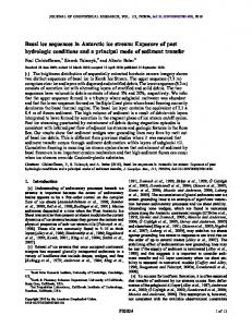
1 – Ice flow across basal thermal transitions

Figure 1.1: Simulated basal temperature distribution in Antarctica. The color scale refer to basal temperature (◦ C) corrected for the pressure-dependence of the melting point. Credit: Pattyn (2010).

small thickness and very cold surface temperature, while becoming warm-based towards the margin as a result of increased strain heating. This is also inferred to occur in Greenland (Dansgaar et al., 1969; Gundestrup & Hansen, 1984). A map of basal temperature from numerical simulations of the Antarctic ice sheet is presented in figure 1.1, which gives an idea of the complexity of the basal temperature field. Looking at smaller spatial scales, similar transitions in basal thermal conditions are observed in correspondence of transition between fast ice stream flow and slow ridge flow in the Siple Coast region of West Antarctica (Retzlaff & Bentley, 1993), and are predicted to occur along their tributaries as well (Vogel et al., 2003). This poses a question about the possible role of basal thermal transitions with respect to the onset of fast ice stream flow and ice stream spatial patterning. The onset of fast ice stream flow is usually ascribed to a thermal feedback where increased heat production (either within ice or at the bed) leads to faster 10

i

i i

i

i

i

i

i

1.1 – Geometry

flow (either via a reduction of viscosity, (e.g., Hindmarsh, 2004) or an increase in bed lubrication (e.g., Fowler & Johnson, 1996b; Sayag & Tziperman, 2009)). A similar feedback results at basal thermal transitions from intense heat dissipation at the transition that favours the formation of basal conditions that permit sliding. This feedback may lead to ice stream formation. Exploring the role of the basal thermal transitions with respect to ice stream formtion is the subject of this part of the thesis. In order to do so, a model describing the evolution of basal thermal transitions as a result of the interaction with the ice flow is needed. To our knowledge, no such model exists in the literature, as the approach devised for numerical ice sheet models appears not to suit our case. In large scale ice sheet models the location of the non-sliding to sliding transition is usually imposed in terms of a variation of the friction coefficient of the bed, with its spatial distribution obtained by inversion of surface velocity data. This procedure ensures a good matching between simulations and the observed, present-day state of the modelled ice sheet, and can thus be used to simulate ice flow evolution on a time scale much shorter than that typical of large scale ice sheet dynamics. Since the position of no sliding to sliding transitions is somewhat constrained by the choice of the friction coefficient rather than modelled, this approach does not allow to address our question, which in essence amounts to asking what are the physical processes leading to spatial patterning in the slipperiness of the ice-bed contact. In the present chapter we derive a model for the large scale flow of ice across basal thermal transitions from first principles. We do so without a priori imposing the position of the transition, which we treat as a moving boundary. We then develop a boundary layer description of heat and mass transport for the region that divides cold-based, and thus slowly flowing ice, from temperate-based, and thus sliding ice. This approach leads to a relationship between the migration rate of the transition and large scale ice sheet variables, such as ice thickness, flux and surface slope. Once obtained, this relation allows us to (i) incorporate the dynamics of the transition in a computationally-efficient, thin-film ice sheet model, and (ii) study the interaction between ice flow and the transition itself. The latter point is the subject of chapter 2.

1.1

Geometry

We consider an ice sheet flowing with velocity u in the positive x−direction, whose geometry is illustrated in figure 1.2. The ice sheet extends from a divide located at 11

i

i i

i

i

i

i

i


x = 0, to its edge located at x = xe (y, t), and has extent L in the horizontal plane. The ice sheet is symmetric with respect to the divide, has thickness h(x, y, t), and rests on a rigid bed. The leading order model that we derive below relies on the consideration that ice sheets are much longer than they are thick (L D, with D a typical ice thickness scale), namely we adopt a thin-film flow model. This is plausible for continental ice sheets: for instance in West Antarctica the distance between the divide and the edges of the ice sheet is roughly 1000 km, with ice thickness between 1 and 2 km, yielding an aspect ratio ε = D/L around 0.005. A basal thermal transition occurs at x = xm (y, t). This transition connects a region where the bed is below the pressure-melting point (denoted in yellow in figure 1.2), and hence ice flows solely by internal deformation, to a region where the bed is at the pressure-melting point (denoted in blue in figure 1.2), and so basal sliding is also allowed. We pose no constraints on the thermal configuration of the ice sheet, which can feature either cold divide and temperate edge or vice versa, depending on the parametric regime under consideration. Sliding is thermally-initiated, in the sense that temperature at the base of the ice sheet determines whether sliding is possible or not. This forces us to consider a thermo-mechanically coupled ice sheet model, because the temperature distribution controls the pattern of basal velocity. Further, the reverse feedback that couples the flow field to the temperature field through strain heating gives to our problem the nature of a free boundary problem. In other words, not only the thermal configuration of the ice sheet, but also the position of the transition is not known a priori, and needs to be determined as part of the solution. The thermal control of sliding initiation raises a question about how the sliding velocity depends on basal temperature. In particular, basal melt water can form even below the pressure-melting point as a result of premelting, thus favouring so-called subtemperate sliding. To start with, we restrict ourselves to the case where sliding is initiated at the location where basal temperature attains the melting point, which we refer to as the hard switch case. Since different boundary conditions at the bed hold depending on whether sliding is possible or not, we consider two separate sub-domains, each of which has extent in the x−direction comparable to the ice sheet length scale, L. We postpone a discussion on the role of subtemperate sliding to chapter 2. 12

i

i i

i

i

i

i

i

1.2 – A Three-dimensional Ice Sheet Model

z

s(x

,y,t

D

h(x,y,t)

)

u

y

u xm

xe

x

L Figure 1.2: Geometry of the ice sheet. The ice sheet flows in the positive x direction. The y−axis is transverse to the flow, and z denotes the vertical direction, positive upwards. The ice divide is located at x = 0, and the edge of the ice sheet at x = xe . The transition between cold (yellow) and temperate (blue) bed occurs at x = xm .

1.2

A Three-dimensional Ice Sheet Model

The three-dimensional flow of ice is described by the Stokes equations ∂τxx ∂τxy ∂τxz ∂p + + − = 0, ∂x ∂y ∂z ∂x ∂τ yx ∂τ yy ∂τ yz ∂p + + − = 0, ∂x ∂y ∂z ∂y ∂τzx ∂τzy ∂τzz ∂p + + − = ρg, ∂x ∂y ∂z ∂z

(1.1a) (1.1b) (1.1c)

where τi j are the components of the deviatoric stress tensor, p is the pressure, ρ is the density of ice, and g acceleration due to gravity. For simplicity, we assume that ice behaves as a Newtonian fluid and viscosity does not depend on the temperature. Therefore, the deviatoric stress tensor depends on the strain rate Di j through the constitutive relation τi j = 2ηDi j ,

(1.2a)

where η is the viscosity and the summation convention applies. The strain rate is linked to the velocity field u = (u, v, w) through ! 1 ∂ui ∂u j Di j = + , (1.2b) 2 ∂x j ∂xi 13

i

i i

i

i

i

i

i


and mass conservation requires that the flow field satisfies ∂u ∂v ∂w + + = 0. ∂x ∂y ∂z

(1.3)

Boundary conditions for the Stokes problem needs to be posed at the ice surface z = s and at the bed z = b. No stress is applied at the ice surface, which yields ∂s ∂s − τxx − p − τxy + τxz = 0, ∂x ∂y ∂s ∂s −τ yx − τ yy − p + τ yz = 0, ∂x ∂y ∂s ∂s −τzx − τzy + τzz − p = 0. ∂x ∂y

(1.4a) (1.4b) (1.4c)

The ice surface evolves according to a kinematic boundary condition ∂s ∂s ∂s +u +v − w = a. ∂t ∂x ∂y

(1.5)

where a is the rate at which mass is accumulated (> 0) or ablated (< 0) at the surface. The ice lies on a layer of sediments or on the bedrock, which is assumed to be the flat surface b = 0. At the bed we have to distinguish between cold (basal temperature below the melting point) and temperate (basal temperature at the melting point) regions of the domain. Where the bed is cold, no slip applies u = 0.

(1.6a)

If instead the bed is temperate, basal melt water allows sliding. In this case we have u · n =0, ui τ jk (δi j nk − ni n j nk ) =τb , |u|

(1.6b) (1.6c)

where (1.6b) assumes no penetration of ice into the bed and no basal melting, while (1.6c) states that the shear stress at the base has the same direction as the velocity vector. n is the normal vector, which for a flat bed is n = (0,0,1) .

(1.7)

14

i

i i

i

i

i

i

i

1.2 – A Three-dimensional Ice Sheet Model

The magnitude of basal shear τb is given by a friction law of the form τb = C|u|1/n ,

(1.8)

which is appropriate to describe viscous creep over small-scale basal roughness (Weertman, 1957; Nye, 1969; Kamb, 1970; Fowler, 1981). Here C depends on the roughness of the bed, and n is the exponent of Glen’s law, which we take equal to one consistently with the assumption of Newtonian ice rheology. Whether or not sliding occurs is determined by the temperature distribution within the ice sheet and the bed, which we need to solve for. Within ice (0 < z < s) we have that temperature evolves according to ! ∂T ρc + u · ∇T + ∇ · (−κ∇T) = τi j Di j ∂t

(1.9a)

while within the bed (−∞ < z < 0) we have ρbed cbed

∂T + ∇ · (−κbed ∇T) = 0 ∂t

(1.9b)

∂ ∂ ∂ , ∂y , ∂z }, the constant c and cbed , κ and κbed with the del operator defined as ∇ := { ∂x the specific heat capacity and thermal conductivity of ice and bed, respectively, and strain heating within ice given by

 ! !2  ∂u 2 ∂v  τi j Di j =2η  + + ∂x ∂y !2 ∂u ∂w +η + +η ∂z ∂x

!2  !2   + η ∂u + ∂v +  ∂y ∂x !2 ∂v ∂w + . ∂z ∂y ∂w ∂z

(1.9c)

We now turn to the boundary conditions for the heat equation. We require that temperature attains a prescribed value on the surface T = Tsur f

(1.10)

and that a constant geothermal heat flux, q geo , is matched in the bedrock far field, −κbed

∂T → q geo ∂z

as z → −∞.

(1.11)

At the bed (z = 0) we have to distinguish between cold and temperate regions. If the bed is cold, no slip occurs at the base and no heat is produced by friction at 15

i

i i

i

i

i

i

i


Table 1.1: Physical constants and scales

Symbol g c κ ρ q geo C η [a] L Tsur f Tmelt

Description (units) gravity acceleration (m s−2 ) specific heat capacity (J kg−1 K−1 ) thermal conductivity (W m−1 K−1 ) ice density (kg m−3 ) geothermal heat flux (W m−2 ) friction coefficient (kPa m−1 yr) viscosity (Pa s) accumulation (m/year) ice sheet length (km) surface temperature (K) melting point (K)

Value 9.81 2 × 103 2.3 917 5 × 10−2 0.5 1012 0.3 3000 240 273

the interface between ice and bed. Therefore, normal heat fluxes in the bed and in the ice must match at the base, that is (−κ∇T · n|+ − (−κbed ∇T · n|− = 0,

and T < Tmelt ,

(1.12a)

with continuous basal temperature [T]+− = 0,

(1.12b)

and the notation ± used hereafter to define the two sides of an interface, with the + sign assigned to the side with positive normal vector. The bed on the temperate side needs to have a non-zero water content in order for the transition between no slip and sliding to occur, in contrast to the frozen side where the water content is zero. This means that melting needs to occur on the temperate side in order to sustain sliding. Hence, here we require a positive net heat flux to the bed, that is (−κ∇T · n|+ − (−κbed ∇T · n|− + τb ub > 0,

and T = Tmelt ,

(1.12c)

where the latter term in the inequality constraint accounts for frictional heating, and the dependence of the melting point on temperature is neglected. In the next section we non-dimensionalise the model, and exploit the assumptions of small aspect ratio and highly conductive ice sheet to derive a simplified leading order approximation. 16

i

i i

i

i

i

i

i

1.3 – Simplified Model

1.3 1.3.1

Simplified Model Non-dimensionalization

We start the process of making our model dimensionless by recognizing that the horizontal length scale, given by the extent of the ice sheet L, is a known quantity, and by fixing the scale for the accumulation rate [a] to a value that characterizes the climatic conditions typical of the ice sheet under consideration. Scales for the horizontal and vertical components of velocity, pressure, stresses and temperature need to be determined. In the following, [·] refers to the scale for the variable in brackets. The purpose of our work is to derive a model for the flow of ice across a basal transition where sliding is thermally initiated. This implies only a moderate amount of sliding is expected to occur on the temperate side of the transition. Hence the mass flux is determined primarily by shear deformation rather than basal sliding. This is tantamount to say that the shear velocity is a suitable scale for the horizontal components of the flow field in both sub-domains. Since ice flow is gravity driven, we balance the horizontal pressure gradient with the vertical gradient of the vertical shear stress, which gives [τxz ]/[z] = [p]/L and [τ yz ]/[z] = [p]/L. Accordingly, we have [τxx ] = ε[τxz ],[τ yy ] = ε[τxz ], [τzz ] = ε[τxz ], and [τxy ] = ε[τxz ]. Mass conservation suggests [w] = [z][u]/L and [u] = [v], while balance of terms in the kinematic boundary condition yields [w] = [a], [u] = [a]L/[z], and [t] = [u]/L, where the latter shows that the relevant time scale is dictated by along-flow advection. The scaling for pressure is then provided by momentum conservation in the vertical direction, whereby we obtain a hydrostatic presure distribution at leading order. Therefore [p] = ρg[z] and [τxz ] = ρg[z]2 /L. The constitutive relationship links the scale for the shear stress to the scale for the horizontal velocity through [τxz ] = η[u]/[z], which allows us to compute the vertical length scale !1/4 η[a]L2 [z] = . (1.13) ρg Scales for velocity, pressure, time and stresses are then computed through the relationships given above. Lastly, a suitable scale for temperature is given by the difference [T] = Tsur f −Tmelt , which is a measure of the conductive heat loss towards the ice surface. Equipped with these scales, the model’s variables are nondimensionalized as x∗ = x/L, z∗ = z/[z], T∗ = (T − Tmelt )/[T], etc. 17

i

i i

i

i

i

i

i


In real situations we expect a small aspect ratio ε = [z]/L, i.e. the ice sheet is shallow. We anticipate that this scaling, along with the assumption of shallowness (ε 1), will lead to a standard ’shallow ice’ model (Fowler & Larson, 1978; Morland & Johnson, 1980). We also note that the mechanical component of the temperate version of the model corresponds to the regime referred to as ’slow sliding (ii)’ in Schoof & Hindmarsh (2010).

1.3.2

A Conductive Ice Sheet Model

We now derive a simplified version of the model based on the assumption of shallowness. Omitting terms of O(ε2 ) and higher, and immediately dropping the asterisks, we obtain that the leading order non-dimensional momentum balance obeys ∂τxz ∂p − = 0, ∂z ∂x ∂τ yz ∂p − = 0, ∂z ∂y ∂p = 1, − ∂z

(1.14a) (1.14b) (1.14c)

while the scaled mass conservation mantains its previous form ∂u ∂v ∂w + + = 0. ∂x ∂y ∂z

(1.15)

The constitutive relation simplifies to ∂u ∂v + = τxy , ∂y ∂x ∂u = τxz , ∂z ∂v = τ yz , ∂z

∂u = τxx , ∂x ∂w 2 = τzz , ∂z ∂v 2 = τ yy , ∂y 2

(1.16a) (1.16b) (1.16c)

which shows that the lateral components of the vertical shear stresses, τxz and τ yz , are o(ε). The boundary conditions on the ice surface now read ∂h + u · ∇h = a + w, ∂t

∂u = 0, ∂z

∂v = 0, ∂z

p = 0,

(1.17a)

18

i

i i

i

i

i

i

i


while at the bed, z = 0, we have u=0 w = 0,

∂v = γv, ∂z

∂u = γu, ∂z

if T < 0,

(1.17b)

if T = 0

(1.17c)

where the non-dimensional friction parameter γ=

C[u] C[a]L2 = [τxz ] ρg[z]3

quantifies the relative importance of basal traction with respect to vertical shear. We now consider the heat equation. Here for simplicity we assume that the bed has the same thermal conductivity as ice. This choice is in line with our objective to gain a qualitative insight on the behaviour of basal thermal transition, although we expect it to have a quantitative effect on the numerical results of the boundary layer model that will be developed in the next section. Under this further assumption, and again neglecting terms of O(ε2 ) and higher, we have  ! ! !2   ∂u 2 ∂v  ∂2 T ∂T  + + u · ∇T − 2 = α  Pe  ∂t ∂z ∂z  ∂z Pe

∂T ∂2 T − 2 =0 ∂t ∂z

for

0 < z < s,

(1.18a)

for

− ∞ < z < 0,

(1.18b)

where only the vertical component of the conductive heat flux survives at leading order, and viscous dissipation results solely by vertical shear stresses. Two non-dimensional parameters appear in the heat equation, namely Pe and α. The Peclet number ρc[z][a] ρcκ−1 [z]2 Pe = = κ [t] compares conductive cooling to heat advection in the horizontal plane through their respective time scales, while the parameter α=

ρg[z]2 [a] [τxz ][u] = κ[T] κ[T][z]−1

is a measure of the relative strength of strain heating with respect to conductive cooling. Turning to boundary conditions, on the surface z = s we obtain T = −1,

(1.19a)

19

i

i i

i

i

i

i

i


while at the bed z = 0 we have [T]+− = 0, " either

∂T ∂z

+ αγ|u|2 > 0

if

T = 0,

(1.19c)

if

T < 0.

(1.19d)

−

" or

(1.19b)

#+ ∂T − ∂z

#+ =0 −

Lastly, in the bedrock far field temperature must satisfy −

∂T →ν ∂z

as z → −∞,

(1.19e)

with ν = q geo [z]/(κ[T]) the scaled geothermal heat flux. The model involves four dimensional groups, namely γ, Pe , α, ν. With the parameters and scales given in table 1.1, they assume the values γ ≈ 20, Pe ≈ 8, α ≈ 2, ν ≈ 1.1. Although simplified with respect to the full Stokes problem, the non-dimensional model is still complicated enough that we are unable to gain any insight about the solution. Difficulties come primarily from the inequality constraints in (1.19). These constraints dictate what sub-set of basal boundary conditions applies to both the mechanical and thermal problems, which is a necessary information to attempt a solution. However, the constraints cannot be evaluated unless the solution of the temperature field is known. This formulation is analogous to the elastic contact problem known as Signorini problem, or, more generally, to obstacle problems (Kinderlehrer & Stampacchia, 1980; Rodrigues, 1987). In order to make further progress, here we assume the asymptotic limit of a highly conductive ice sheet (i.e., Pe 1), which allows for an explicit integration of the large scale temperature field. This assumption is not intended to be strictly realistic, as a moderately large Pe means that along-flow heat advection affects the temperature field of an ice sheet significantly. However, we anticipate here that the rescaling in the boundary layer region across the transition is such that advective terms are brought back to leading order in the heat equation, which features a balance between internal heating, along flow and vertical advection, and heat diffusion in vertical planes. In other words, we maintain an O(1) Peclet number locally in correspondence of the mechanical boundary layer, with the idea that heat production and transport in this region are a leading order control on the dynamics of the contact line, but we disregard the effects of advective heat transport in the far field. An alternative approach, as well as the implications of taking Pe 1, are discussed in section 1.5. 20

i

i i

i

i

i

i

i


Integration The simplified mechanical model (1.14) can be integrated straightforwardly between z = 0 and z = h to obtain the pressure and velocity fields (Fowler & Larson, 1978; Morland & Johnson, 1980). (1.14)3 with (1.17a)4 immediately yields a hydrostatic pressure distribution p = h − z. By substituting the expression for pressure into (1.14)1,2 , and integrating over the ice thickness using the constitutive relationships (1.16) as well as the boundary conditions (1.17a)2,3 , and either (1.17c) or (1.17b), we obtain the following solution for the horizontal velocity vector uh = (u, v) either or

i 1h 2 h − (h − z)2 ∇h h 2 " 2 # h − (h − z)2 h uh = − + ∇h h 2 γ uh = −

if T = 0 at z = 0,

(1.20a)

if T < 0 at z = 0,

(1.20b)

with ∇h = (∂/∂x, ∂/∂y). We can now integrate mass conservation (1.15) over the ice thickness, and imposing bed impermeability we obtain the vertical velocity ! z z3 z2 + ∇h 2 h2 − ∇h 2 h if T = 0 at z = 0, (1.21a) either w= 4 2γ 6 or

w=

z2 2 2 z3 2 ∇h h − ∇h h 4 6

if T < 0 at z = 0.

(1.21b)

Finally, depth-integration of mass conservation and substitution into the kinematic boundary condition (1.17a)1 yields the evolution equation for the ice thickness ∂h + ∇h · q = a, ∂t

(1.22)

which is indeed a diffusion equation for the ice flux h

Z q=

uh dz = −Q(h, | ∇h h|) 0

∇h h . | ∇h h|

(1.23)

Here Q is the diffusion coefficient, which depends on the basal thermal conditions as ! 1 3 1 2 if T = 0 at z = 0, (1.24a) either Q = h + h | ∇h h| 3 γ 1 or Q = h3 | ∇h h| if T < 0 at z = 0. (1.24b) 3 21

i

i i

i

i

i

i

i


We now turn the attention to the thermal problem, which under the assumption of small Pe reads ∂2 T = (h − z)2 | ∇h h|2 ∂z2 ∂2 T − 2 =0 ∂z

−

for

0 < z < h,

(1.25a)

for

− ∞ < z < 0,

(1.25b)

whereas the boundary conditions remain unaltered. The equations above illustrate that, by taking the limit of a highly conductive ice sheet, we assume that the temperature field adjusts instantly to changes in the geometry of the ice sheet through a balance between strain heating and conductive cooling, where the strain heating term originates solely by vertical shearing. This problem can be integrated straightforwardly between z = b and z = s with boundary conditions (1.19) to show that temperature depends only on the local ice thickness and surface slope. We find that in the cold bed case, the temperature distribution satisfies # "   (h − z)4 α  2 3 4   |∇h h| − − zh + h + ν(h − z) − 1 for 0 < z < h,  3 4 (1.26a) T=   α   for − ∞ < z < 0,  |∇h h|2 h4 + ν(h − z) − 1 4 while for the temperate case we have  α h i z  2 4 3 4    12 |∇h h| −(h − z) − zh + h − h T=    − νz

for

0 < z < h,

for

− ∞ < z < 0.

(1.26b)

Given the temperature distribution, the inequality constraints in (1.19) can be expressed in terms of the same variables that appear in the diffusion problem (1.22), namely ice thickness and flux, as ! 3 1 1 2 2 h either − + ν + α |∇h h| + h > 0 if T = 0 at z = 0, (1.27a) h 4 γ α or −1 + νh + |∇h h|2 h4 < 0 if T < 0 at z = 0. (1.27b) 4 After integrating the flow and temperature fields, we are left with a diffusion problem for the ice thickness (1.22) constrained by the inequalities 1.27a, where the non-constant diffusion coefficient Q assumes different forms depending on the thermal conditions at the base of the ice sheet. If a thermal transition is to 22

i

i i

i

i

i

i

i


occur at x = xm , then (1.22) holds in each sub-domain, namely 0 < x < xm and xm < x < xe , with the relevant diffusion coefficient given by (1.24a). Suitable boundary conditions must then be given at the edges of the domain, namely the divide and the edge of the ice sheet, as well as at the boundary between each sub-domain, where the transition occurs. The ice sheet is assumed symmetric with respect to the divide x = 0, hence we ask no normal flux q⊥ = q · n = 0 at x = 0. (1.28a) At the transition x = xm the ice thickness needs to be continuous, and mass conservation in the direction normal to the transition must be ensured, hence we ask + q⊥ − = 0, [h]+− = 0 at x = xm (1.28b) Finally, at the margin of the ice sheet x = xe we have two possible configurations. For a land-based ice sheet, the margin is defined as the location where flux and thickness vanish simoultaneously, i.e. Z xe a(x) dx = 0, and h = 0 at x = xe . (1.28c) 0

In this case we also need to account for a spatially-dependent accumulation rate, as the position of the margin is implicitely defined by the surface mass balance. Alternatively, we can consider a marine ice sheet. The edge of a marine ice sheet corresponds to the grounding line, where suitable boundary conditions prescribe that the ice must be at flotation and the flux is a function of the depth to bed. Mathematically, we have h=−

ρwater b, ρ

and

q⊥ = Q g (h)

at

x = xe ,

(1.28d)

where b is a bed profile below sea level, and the function Q g is a power-law whose exponent depend on whether no slip or sliding occur at the grounding line (Schoof, 2007, 2011; Chogunov & Whilchinsky, 1996). The necessity of a boundary layer We note that the position of the transition is not known, and we also anticipate (see section 2.1) that the inequalities (1.27a) do not provide sufficient information to constrain it. In addition, the hard switch between non-sliding and sliding regimes is known to cause a discontinuity in the horizontal velocity and a singularity in the stress field (Fowler, 2001). 23

i

i i

i

i

i

i

i


The discontinuity in horizontal velocity can be easily recognized by considering the simple case of a one-dimensional transition. In this case conservation of normal flux across the transition implies a jump in surface slope 1/3h3 dh dh , = dx warm 1/3h3 + h2 /γ dx cold

(1.29)

which substituted into the solution for the horizontal velocity (1.20a) yields clearly a jump in the horizontal velocity. These shortcomings indicate that a smaller scale description of the stress field, as well as of heat production and transport across the transition, is needed to capture the dynamical behaviour of the transition and its interaction with the flow field. Mathematically, this region can be treated as a boundary layer. A boundary layer model describing the coupled heat and mass transport across a basal thermal transition is derived in the next section. Beside ensuring a smooth transition between non-sliding and sliding regions of an ice sheet, the boundary layer will also provide an evolution equation for the position of the basal transition. This equation relates physical processes taking place at the small boundary layer scale to large scale variables such as ice thickness and flux, and therefore serves as a physically-based parametrization of the boundary layer physics suitable to be implemented in a large scale ice sheet model.

1.4

The Boundary Layer

Boundary layer problems arise quite commonly in glaciology, for example in the study of ice stream shear margins (Haseloff et al., 2015) or of the grounding zone of marine ice sheets (Chogunov & Whilchinsky, 1996; Schoof, 2007, 2011). The model we derive here is similar to that by Haseloff et al. (2015), which describes the thermo-mechanical boundary layer that connects slowly flowing ice ridges with fast flowing ice streams. The fundamental difference is that, in their case, ice flow in the temperate domain (ice stream)is parallel, rather than normal, to the boundary layer. Differently, here we consider either the case of no tangential flux, or the case of comparable ice fluxes in the directions normal and tangential to the boundary layer. This holds implications for heat production in the boundary layer and, hence, for the dynamical behaviour of the transition that we will discuss further in chapter 2. A further difference is that we require a limited amount of sliding on the temperate side of the transition, rather than free slip like in the shear margin case. A 24

i

i i

i

i

i

i

i

1.4 – The Boundary Layer

model addressing this situation has been previously proposed by Bueler & Brown (2009b), where solutions of the non-sliding shallow ice model are heuristically weighted with solutions of a so-called ’shallow-shelf’ model (a thin-film model with free slip at the base) to simulate a smooth transition between no-slip regions. Here we pursue a different angle: by treating the transition as a boundary layer, we derive a model that allows to retain those components of the stress tensor that are responsible for a smooth transition between no slip and sliding only in the narrow region where they are expected to be significant. The boundary layer formulation ensures matching with the regions upstream and downstream of the boundary layer, where simpler -and computationally-efficient- descriptions of the flow and temperature field are known to be valid.

1.4.1

Problem Formulation

To illustrate the derivation, we consider the case of an ice sheet uniform in the direction parallel to the transition, whereas the model for the case with non-zero tangential flux is stated in appendix A.1. The boundary layer is located between the cold and temperate sub-domains, in the region that we call contact line at x = xm . Here basal temperature has to reach the melting point, in order for the flow to transition from a Poiseuille flow to a shear flow that experiences a limited amount of slip at the wall. The boundary layer needs not to be shallow, otherwise the same stress balance as in the outer problem would apply, and the stress singularity at the contact line would not be healed. Hence, we introduce a rescaling for the along-flow coordinate at the ice thickness scale, namely X=

1 [x − xm (t)] , ε

(1.30)

so that the boundary layer is always centered on the contact line. The boundary layer along-flow coordinate now spans the interval −∞ < X < +∞. Mass conservation suggests [W] = ε[w], where capital letters refer to boundary layer variables. In addition, we expect compressive and extensional stresses to be comparable with shear stresses, and thus we put [Txx ] = ε[τxx ], [Tzz ] = ε[τzz ]. The remaining variables are unscaled, hence [P] = [p] and [TBL ] = ε[T]. By substituting these scales in the outer problem, we obtain the following boundary layer problem. 25

i

i i

i

i

i

i

i


Momentum conservation reads ! ∂Txx ∂Txz ∂P + =0, ε − ∂X ∂Z ∂X ! ∂Txz ∂Tzz ∂P ε + =1, − ∂X ∂Z ∂Z

(1.31a) (1.31b)

with the constitutive relationship now yielding ∂U , ∂X ∂U Tzz = 2 , ∂X ∂U ∂W Txz = + . ∂Z ∂X Mass conservation can be expressed as Txx = 2

∂U ∂W + = 0. ∂X ∂Z The boundary conditions on the ice surface Z = H are −(ετxx − P)

∂H + εTxz = 0, ∂X

∂H + εTzz − P = 0, ∂X ∂H dxm ∂H ∂H ε − +U − W = εa, dt ∂X ∂t ∂X while at the bed Z = B we have −εTxz

W = 0, U=0

(1.32a) (1.32b) (1.32c)

(1.33)

(1.34a) (1.34b) (1.34c)

(1.35a) for

X < 0,

(1.35b)

∂U = γU for X > 0. (1.35c) ∂Z Note that here we specify that subdomain upstream of the contact line is coldbased, while the downstream one is temperate-based. However, the thermal configuration is effectively dictated by the outer problem, and the reverse configuration is equally possible. We now turn to the thermal problem. Within ice (0 < Z < H), the heat equation becomes ! ! dxm ∂TBL ∂TBL ∂TBL ∂2 TBL ∂2 TBL Pe BL − +U +W − + = α ΦBL , (1.36a) dt ∂X ∂X ∂Z ∂X2 ∂Z2 26

i

i i

i

i

i

i

i


with the boundary layer parameter Pe BL = ε−1 Pe , and the strain heating term now reading !2 !2 !2 ∂U ∂W ∂U ∂W + ΦBL = 2 +2 + . (1.36b) ∂X ∂Z ∂Z ∂X In the bed (−∞ < Z < 0) we obtain −Pe BL

! ∂2 TBL ∂2 TBL dxm ∂TBL − + = 0. dt ∂X ∂X2 ∂Z2

(1.36c)

Although our scaling suggests that Pe is a moderately large parameter, to simplify our analysis we have previously assumed that Pe 1. This however poses the question of how should we treat the boundary layer parameter Pe BL . Here we will consider Pe BL an O(1) parameter, meaning that at the ice sheet length scale the effect of heat advection on the temperature field is comparable to that of (vertical and horizontal) heat conduction and strain heating. Turning to the boundary conditions, at the surface we find TBL = −1,

(1.37a)

while at the bed boundary conditions read [TBL ]+− = 0,

either " or

TBL = 0 #+ ∂TBL − =0 ∂Z −

(1.37b)

for

X > 0,

(1.37c)

for

X < 0,

(1.37d)

and in the bedrock far field −

∂TBL →ν ∂Z

as Z → −∞.

(1.37e)

Finally, the following inequality constraints must also hold "

∂TBL ∂Z

#+ + U2 αγ > 0

for

X > 0,

Z=0

(1.38a)

TBL < 0

for

X < 0,

Z = 0.

(1.38b)

−

27

i

i i

i

i

i

i

i


1.4.2

Series Expansion

Aiming at finding a leading order solution for the velocity and temperature field and for surface elevation, we now pose the following asymptotic expansions in ε P(X, Z, t) = P0 (X, Z, t) + εP1 (X, Z, t) + o(ε), H(X, t) = H0 (X, t) + εH1 (X, t) + o(ε), U(X, Z, t) = U0 (X, Z, t) + o(1), W(X, Z, t) = W 0 (X, Z, t) + o(1), 0 TBL (X, Z) = TBL (X, Z) + o(1).

We start from considering momentum conservation in the vertical direction, which at zeroth order reads ∂P0 = −1, ∂Z which is to be integrated over the ice thickness with (1.34b). To evaluate pressure at the surface we expand pressure at the surface in Taylor series as " 0 # ∂P (X, H0 , t) 1 0 0 1 0 P(X, H, t) = P (X, H , t) + ε H (X, t) + P (X, H , t) + o(ε2 ), ∂Z which used as boundary condition for the vertical momentum balance yields a hydrostatic pressure distribution P0 = H0 − Z at zeroth order. By substituting the pressure distribution in the horizontal momentum conservation, we obtain that the ice surface is flat at leading order, namely ∂H0 = 0. ∂X The boundary layer therefore occupies a rectangular region spanning −∞ < X < +∞ in the horizontal direction and 0 < Z < H0 in the vertical direction. U and W are therefore solution to the Stokes problem ∂2 U0 ∂2 U0 ∂P1 = 0, + − ∂X ∂X2 ∂Z2 ∂2 W 0 ∂2 W 0 ∂P1 = 0, + − ∂Z ∂X2 ∂Z2

(1.39a) (1.39b)

subject to boundary conditions ∂U0 ∂W 0 + = 0, ∂Z ∂X

W 0 = 0,

2

∂W 0 + P1 = H 1 ∂Z

at

Z = H0

(1.40a)

28

i

i i

i

i

i

i

i


on the ice surface, and W 0 = U0 =0 W0 =

∂U0 − γU0 =0 ∂Z

for X < 0,

Z = 0,

(1.40b)

X > 0,

Z = 0,

(1.40c)

for

at the bed. The thermal problem remains identical to (1.36).

1.4.3

Matching

To complete the mathematical problem, boundary conditions need to be posed on the vertical boundaries of the boundary layer at X → ±∞. This is indeed the matching region, and boundary conditions posed here serve to ensure that the boundary layer problem matches the outer, large-scale problem on both sides. To facilitate this task, we recall that the following scale relations between inner and outer variables hold, ε[X] = [x] − xm (t), [U] = [u],

[Z] = [z],

[W] = ε[w],

[Txx ] = [Tzz ] = ε[τxz ],

[P] = [p],

[Txz ] = [τxz ],

[TBL ] = [T], and start by considering the constraints given by the boundary conditions for the outer problem at the contact line, where the boundary layer is located. Boundary conditions (1.28b) posed at x = xm require continuous ice thickness and normal flux at the contact line. The former implies that the ice thickness in the boundary layer is dictated by the outer problem through lim h = lim+ h = H0 ,

x→x−m

(1.41)

x→xm

whereas flux continuity is ensured if H0

Z

H0

Z U dz = lim 0

lim

X→−∞

X→+∞

0

U0 dz. 0

By integrating mass conservation over the ice thickness we obtain that the rate of change of the flux in the boundary layer is ∂ ∂X

H0

Z 0

H0 U0 dZ = − W 0 0 , 29

i

i i

i

i

i

i

i


where the right hand side vanishes according to boundary conditions (1.40a)2 , and either (1.40b)1 or (1.40c)1 . Flux conservation is therefore ensured. The normal flux that moves across the boundary layer is provided by the outer problem, and depends on the position of the contact line as Z H0 Z xm 0 0 q = U dz = a dx. 0

0

Aided by the scale relationships above, we now turn to the velocity field. Here, we require that U0 → u as X → ±∞ and W 0 → 0 as X → ∞. With the outer solution given by (1.20a) and the jump condition for surface slope at the contact line (1.29), matching conditions for the horizontal velocity read  2 3q0  1  0 0 2 0  U ∼ (H ) − H − Z for X → −∞,    2 (H0 )3      2     (H0 )2 − H0 − Z 0  3γq0 H (1.42a)      U0 ∼  + for X → +∞,   0 3 0 2   2 γ  γ(H ) + 3(H )         W0 → 0 for X → ∞, which supplement the boundary conditions for the Stokes problem (1.39). Moving to the temperature fields, matching conditions need to ensure that TBL → T as X → ∞. With the outer solution given by (1.26), within ice (B < Z < S0 ) we have # !2 " (H0 − Z)4 α 3q0 0 3 0 4 0 0 − Z(H ) + (H ) + ν H − Z −1 (1.42b) TBL ∼ − 3 (H0 )3 4 on the cold-side of the boundary layer (X → −∞), while matching towards the temperate side (X → +∞) requires !2 i Z h 3γq0 α 0 0 4 0 3 0 4 TBL ∼ −(H − Z) − Z(H ) + (H ) − 0. (1.42c) 12 γ(H0 )3 + 3(H0 )2 H Finally, in the bed (−∞ < Z < 0) we find 0 0 TBL ∼ −νZ + TBL (Z = 0+ )

1.4.4

for X → ∞.

(1.42d)

Implications for the Large Scale Problem

The boundary layer problem as stated in section 1.4.2, along with the matching conditions given in section 1.4.3, is a travelling wave problem whose solution 30

i

i i

i

i

i

i

i


propagates at speed dxm /dt, which we refer to as ’migration velocity’. Solving the boundary layer problem therefore means finding the dependence of the migration velocity on the outer problem’s parameters. Similarly to Schoof (2012) and Haseloff et al. (2015), to facilitate this task we introduce a further rescaling that absorbs the ice thickness H0 and the influx q0 into a minimal number of parameters. Therefore, we pose X , H0

P∗ =

(H0 )2 1 P, q0

H0 (U∗ , W ∗ ) = U0 , W 0 0 , q

vm =

dxm H0 . dt q0

Z∗ =

Z , H0

X∗ =

By subtracting the background conductive profile, we also define a reduced temperature 0 ∗ TBL = −(1 − H0 ν) − νZ + (1 − H0 ν)TBL .

Dropping asterisks hereafter, the boundary layer problem for the flow field becomes ∂2 U ∂2 U ∂P = 0, + − ∂X2 ∂Z2 ∂X ∂2 W ∂2 W ∂P + − = 0, ∂Z ∂X2 ∂Z2

(1.43a) (1.43b)

with boundary conditions ∂U ∂W + =W=0 ∂Z ∂X W=U=0

W = 0,

for

∂U = γ∗ U ∂Z

on Z = 1,

X < 0,

for

Z = 0,

X > 0,

 h i 3   1 − (1 − Z)2    2 " # U→  3 γ0 2  2    2 γ0 + 3 1 − (1 − Z) + γ0

Z = 0,

(1.43c)

(1.43d)

(1.43e)

for X → −∞ for X → +∞

(1.43f)

31

i

i i

i

i

i

i

i


Turning to the thermal problem, within ice (0 < Z < 1) we have !# " ∂TBL ν0 ∂TBL ∂TBL +U +W − + = Pe 0BL −vm 1 − ν0 ∂X ∂X ∂Z ! ∂2 TBL ∂2 TBL + + α0 ΦBL , ∂X2 ∂Z2

(1.44a)

while in the bedrock (−∞ < Z < 0) ∂TBL ∂2 TBL ∂2 TBL = + . ∂X ∂X2 ∂Z2 Finally, boundary conditions simplify to −Pe 0BL vm

TBL = 0 [TBL ]+−

∂TBL = − ∂Z "

TBL = 1

(1.44b)

on Z = 1,

(1.44c)

#+ = 0,

for

X < 0,

X > 0,

Z = 0,

Z = 0,

(1.44d)

−

for

(1.44e)

∂TBL → 0 for Z → −∞, ∂Z # "  4  (1 − Z)  0  −Z+1 for X → −∞ 3α −    4  TBL →   i  3 α0 (γ0 )2 h  4   −(1 − Z) − Z + 1 −Z+1 for X → +∞  4 (γ0 + 3)2 The non-dimensional parameters Pe0BL , α0 , ν0 and γ0 are defined as !2 q0 α Pe 0BL = q0 Pe BL , α0 = , γ0 = H0 γ, ν0 = H0 ν, 1 − ν0 H0 −

(1.44f)

(1.44g)

(1.45)

where Pe BL , α, ν, and γ are known quantities, while H0 and q0 are outer problem variables depending on the position of the boundary layer in the outer domain. The mathematical problem therefore consists of solving the flow problem (1.43), which can be done numerically, and then finding vm subject to the temperature problem (1.44), and to the inequality constraints TBL < 1 " #+ ∂TBL + α0 γ0 U2 > 0 ∂Z −

X < 0,

Z = 0.

for X > 0,

Z = 0.

for

(1.46)

32

i

i i

i

i

i

i

i

1.5 – Discussion

In other words, beside obtaining the flow and temperature fields, the objective is to determine the function that links vm to the boundary layer parameters, 0 vm = Vm Pe 0BL , α0 , γ0 , ν0 , (1.47a) or, in the case of large scale flow not normal to the transition (see appendix A.1), 0 v m = Vm Pe 0BL , α0 , γ0 , ν0 , β0 , (1.47b) where the parameter β0 = ((H0 )3 /q0 |∂H0 /∂Y|)2 accounts for surface slope in the direction parallel to the contact line, and hence, for the flux shearing the boundary layer. Assuming for now that this relation exists, then we can write it in terms of large scale variables. Once the outer problem parameters α, γ, and ν are assigned, the relations above yield ∂xm = Vm (h, q⊥ , | ∇h hk |2 )n, ∂t

(1.48)

where xm = (xm , y), ∇h hk = ∇h h · (I − nn), and n is the vector normal to the contact line and pointing in the positive x−direction. The latter relation is an evolution equation for the contact line, which is here treated as a moving boundary. It complements the large scale problem for ice flow across basal thermal transitions derived in section (1.3.2) by providing an additional constraint on the position of the contact line. Since it describes the motion of the contact line as a function of the outer problem variables ice thickness, flux, and surface slope, it allows to explore the interactions between ice flow and the contact line itself.

1.5

Discussion

In this chapter we have derived a simple, depth-integrated, thermomechanically coupled ice sheet model suitable to describe the large scale flow of ice across basal thermal transitions. The boundary layer treatment of the transition between cold and temperate based ice on the one hand ensures that a shallow ice description of ice flow can be adopted on both sides without resulting in a stress singularity at the transition itself. On the other hand, it yields the desired relationship between the migration velocity of the transition and large scale variables. 33

i

i i

i

i

i

i

i


The fundamental assumption in the derivation of our model is that the global Peclet number is small, which does not strictly apply to real ice sheets. From a physical perspective, restricting ourselves to this case influences the large scale pattern of basal temperature. This is because downwards advection of cold ice tends to counteract strain heating in the ice column, thus less heat reaches the bed. Consequently, either lower temperature (cold side) or smaller heat flux (temperate side) are needed to match basal boundary conditions. In general, we may expect this effect to be more severe on the cold side, as frictional heating provides an additional source of basal heating once the melting point is attained. If the global Peclet number was taken as a O(1) parameter, one consequence in the large scale problem would be that the cold region could persist with larger ice flux, thus the position in space of the contact line would likely differ from the one predicted by a model with small Peclet number. As for the boundary layer region, a rescaling at the ice sheet thickness would yield a purely advective thermal boundary layer of width ε. At least in the case of ice flowing from cold to warm bed, temperature on the cold side should be already very close to melting when the flow enters the boundary layer in order for the transition to occur, meaning that the dynamics of the transition would not ensue from physical processes occurring in this region, but rather from a wider region where heat advection, heat production and strain heating are equally important. Asymptotically, a moderately large global Peclet number appears to support a nested boundary layer description of heat production and transport, with a balance between heat diffusion and internal heating in the region close to the divide, where flow velocity is very low; a larger boundary layer (scaling as Pe −1 ) where the dominant balance is between advection, vertical diffusion and internal heating; a purely advective thermal boundary layer in correspondence of the mechanical boundary layer. Reassured by the fact that even in this case the dynamics of the contact line appears to be determined by a dominant balance in the heat equation which includes advection, internal heating, and heat diffusion in the X, Z plane, similarly to the small Peclet number case, we leave this improvement for future work, and focus on the small Peclet case. The relation (1.48) is actually analogous to a Stefan condition in phase change problems (e.g., Crank, 1984). Keeping with this analogy, the contact line mirrors the boundary between the two phases of a melting solid, which are here represented by the cold and temperate subdomains. In the classical Stefan problem the rate of melting or freezing is given by a mismatch between incoming and outgoing heat fluxes at the interface between the two phases. In our problem, this corresponds to the function Vm , which is essentially a physically-based parametrisation of 34

i

i i

i

i

i

i

i

1.5 – Discussion

the small-scale processes occurring in the boundary layer. Once obtained, the boundary layer model does not need to be solved anymore. This is key to capturing the evolution of basal thermal transitions as a moving boundary in a diffusion problem for the ice thickness h. The analogy to a Stefan problem suggests that the contact line may undergo a morphological instability. In the next chapter we first study the constraints on steady state solutions of the model, and then address the issue of the stability of the contact line to small amplitude perturbations by means of a linear stability analysis.

35

i

i i

i

i

i

i

i

36

i

i i

i

i

i

i

i

Chapter 2

Stability of Basal Thermal Transitions In chapter 1 we have derived a boundary layer model for the flow of ice across basal thermal transitions. In the model, basal thermal transitions are treated as moving boundaries, whose dynamics are described in the outer problem by a Stefan-like boundary condition of the form ∂xm = Vm n. ∂t The function Vm , which describes the migration velocity of the transition in terms of the large scale variables ice thickness, flux and surface slope, is to be determined numerically by solving the boundary layer problem. Here we first present results from the large scale model that constrain the existence of steady state solutions (section 2.1), and then show that the boundary layer model can be solved in the parametric regime where steady state solutions are possible (section 2.2). These results allow us to study the stability of basal thermal transitions to infinitesimal perturbations, which we do with a linear stability analysis for short wavelength perturbations (section 2.3). An instability of the contact line is detected, and the implications for ice stream formation are discussed in section 2.4. 37

i

i i

i

i

i

i

i

2 – Stability of Basal Thermal Transitions

2.1

Steady States

Steady solutions of the large scale model obey ∇ · q = a,

(2.1a)

q = −Q(h, |∇h|)∇h/|∇h|,

(2.1b)

with the gradient operator restricted to the horizontal plane throughout the chapter. The diffusion equation above holds in each sub-domain, namely 0 < x < xm and xm < x < xe , xm being the location of the contact line that divides the cold-based sub-domain from the temperate-based one. In the absence of a contact line, one-dimensional solutions to (2.1), with no sliding at the base and subject to no flux conditions at the divide and at the edge are known to exist, and lead to the so-called Vialov’s profile for the surface elevation (Vialov, 1958). Modified versions of this surface profile can be obtained also for the case with moderate basal sliding, as well as for different boundary conditions at the edge like those outlined in section (1.3.2). Our main concern here is with understanding whether a steady solution exists for the case with basal thermal transitions, possibly in the form of a combination of known one-dimensional solutions that hold in the absence of basal thermal transitions, or in two horizontal dimensions. To this aim, we start our analysis by outlining the key differences with respect to the case of an ice sheet underlain by a cold (or temperate) bed throughout.

2.1.1

Multivaluedness of the Flux Law

We first examine the role of the inequality constraints for basal thermal conditions. To this aim, we note that the flux function Q in the diffusion equation (2.1a) takes slightly different forms in each subdomain. In fact, Q serves as diffusion coefficient, which is to be chosen according to basal thermal conditions. Recalling that for the hard switch case no slip occurs where basal temperature is below the melting point, while thermally-controlled sliding can be sustained only where basal heat production is positive, we find the following expressions for the diffusion coefficient: either or

1 3 h |∇h| 3 ! 1 3 1 2 Q = h + h |∇h|, 3 γ Q=

if − 1 + νh + if −

1 + ν + α |∇h|2 h

α |∇h|2 h4 < 0, 4 ! h3 1 2 + h ≥ 0, 4 γ

(2.2a) (2.2b)

38

i

i i

i

i

i

i

i

2.1 – Steady States

where the above formulation of the inequality constraints apply as a result of the assumption of highly conductive ice sheet. The inequality constraints in (2.2) limit the interval of ice thickness h and surface slope |∇h| for which each branch of the flux law (2.1b) is viable. Whether the intervals overlap or not determines if a steady state solution is in principle possible, as the transition between the two branches of the flux law needs to occur at constant ice thickness. A further condition is prescribed by the continuity of normal flux, which requires a jump in surface slope in the direction normal to the transition. The implication of this further constraint on the existence of steady state solutions is discussed in section 2.1.2. We first examine the overlap of the branches of the flux law, and start by taking h fixed. The cold branch is accessible provided 4(1 − hν) , αh4

|∇h|2
0, we obtain the ratio q− q+

!2 =

(1 + 3ξ)2 , 1 + 4ξ

(2.4)

which needs to be less than one for the flux to be multivalued. We have that (1 + 3ξ)2 = 1 + 4ξ when ξ = 0 and d d (1 + 3ξ)2 = 6 + 18ξ > (1 + 4ξ), dξ dξ so we can conclude that q− /q+ > 1, and no overlap is possible with any ξ. In other words, for any fixed ice thickness there are values of |q| which cannot be generated by any surface slope |∇h|. We refer to this as a ’gap’ in the flux law. The physical interpretation of the gap is related to energy dissipation, which for ice flow is given by strain heating within ice and frictional heating at the bed. Total dissipation in the flow corresponds to the rate of loss of potential energy, q · ∇h. For the warm branch a given flux requires a smaller surface slope ∇h = q/(1/3h3 +h2 /γ) than for the cold branch, where ∇h = q/(1/3h3 ). Hence, counterintuitively we find that at constant flux the cold branch dissipates more heat than the temperate branch. This is because dissipation by strain heating, (h − z)|∇h|2 , is smaller on the temperate side as a result of reduced surface slope, and frictional heating at the bed is not large enough to offset larger dissipation on the cold branch. As a result the warm branch, which requires more heat to keep the bed temperate, can only exist for values of the flux larger than those at which the cold branch persists. A major consequence of the gap is that no one-dimensional steady state is possible that involves both cold and temperate bed. In fact, in this case the flux vector is necessarily normal to the contact line, hence q must be continuous there. The absence of multivaluedness of q means that no transition can possibly occur at an arbitrary location on the branches of the flux law, and if q were to reach the endpoint of one of the branches, then no surface slope would generate the same flux on the other branch.

2.1.3

Oblique Basal Transitions

If the contact line is at an angle with respect to the flow, the gap in the flux law can potentially be bridged as a result of strain heating in the lateral flow. This is because a non-vanishing surface slope in the direction parallel to the transition implies a discontinuity in tangential flux. Since at the transition we now require continuity of normal flux rather than continuity of q, the gap in |q| can possibly be bridged 42

i

i i

i

i

i

i

i


q-

n φ

q+

Figure 2.2: Oblique basal transition with ice flowing from warm- (-) to cold-based (+) ice. The thick black line is the boundary between the two sub-domains and n denotes the normal vector. Flux vectors are solid thick (blue for warm-based, yellow for cold-based), the normal component q⊥ is dashed, and the tangential component qk is solid thin. Note the discontinuity in the tangential component of the flux vector, which is necessary to maintain an oblique basal transition.

if tangential flux components are large enough at the transition. Physically, strain heating due to tangential flow supplies the heat necessary to render the warm branch accessible for a flux small enough that the cold branch can persist. To pursue this angle, the first question we need to answer is how large tangential surface slope needs to be in order for tangential flux to supply the heat necessary to maintain the oblique transition at work. To this aim we consider a two-dimensional steady state with a contact line at an angle ϕ with the flow (as illustrated in figure 2.2), with continuity of ice thickness and normal flux holding at the transition. The key point is that continuity of normal flux implies a jump in surface slope in the direction normal to the transition, whereas surface slope needs to be continuous in the direction parallel to the transition itself. To answer the question above we actually need to find how large the tangential flux must be so that the gap in the flux described by (2.4) can be bridged. Denoting with + quantities on the warm branch of the flux law and with − quantities on the cold branch, we find that continuity of tangential surface slope implies a jump in tangential flux q−k = 1 + 3ξ, (2.5a) q+k whereas

q−⊥ = 1. q+⊥

(2.5b)

43

i

i i

i

i

i

i

i


Aided by the relations above, we can find an expression of the ratio |q− |2 /|q+ |2 that involves the tangential surface slope through the tangential component of the flux. By substitution, we obtain (q−k )2 + (q−⊥ )2 (q+k )2 |q− |2 2 = = 1 + (9ξ + 6ξ) , |q+ |2 (q+k )2 + (q+⊥ )2 |q+ |2 which can be simplified further by specifying that the angle ϕ between flow and transition is taken such that q⊥ = |q| sin ϕ, qk = |q| cos ϕ. As a result, we obtain the following expression for the jump in |q| across the transition |q− |2 = 1 + (9ξ2 + 6ξ) cos2 ϕ, (2.6) |q+ |2 which needs to be larger than the gap (2.4) for a two-dimensional steady solution with a basal thermal transition to exist. Mathematically, we have q− 1 + (9ξ + 6ξ) cos ϕ > + q 2

!2

2

=

(1 + 3ξ)2 . 1 + 4ξ

Solving for the angle between cold flux vector and transition, we obtain r 1 + 2/(9ξ) + + 0 ≤ ϕ < ϕ , ϕ := arccos , (1 + 4ξ)(1 + 2/(3ξ))

(2.7)

whereas an upper bound for the angle between warm flux vector and transition, can be determined through (2.5) as a function of ϕ+ . Physically, when ϕ satisfies the constraint above, heat dissipation due to larger tangential flow on the warm side supplies the heat necessary to make the warm branch accessible at values of |q| where the cold branch still persists. The constraint on the angle between flow and transition provides a lower bound for the boundary layer parameter β0 =

h3 q⊥

!2 ∂h ∂s ,

which quantifies the effect of lateral shear on strain heating in the boundary layer. Here s is the direction parallel to the contact line, which in case of an oblique 44

i

i i

i

i

i

i

i


transition is no more aligned to the y−axis. We now seek the dependence of β0 on ϕ. Considering that on the cold side 1 ∂h q+k = h3 3 ∂s and that normal and parallel flux components are geometrically related, we can express β0 as a function of the angle between flow and contact line as β0 =

3 tan ϕ

!2 ,

(2.8a)

or in terms of warm side variables 3 β = (1 + 3ξ) tan ϕ∗ 0

!2 ,

(2.8b)

where ϕ∗ is the angle between warm flux vector and transition. The two expressions for β0 can be proved to be equivalent using the relations (2.5). Since β0 is a decreasing function of ϕ, then the upper bound for the angle is a lower bound for β0 , i.e. 0

β >β 0

−

3 := tan ϕ+

!2 =

9(2 + 9ξ) . 4(1 + 3ξ)2

(2.9)

A value of β0 fulfilling this constraint ensures that the gap in the flux law can be bridged as a result of heat production due to the discontinuity in tangential flux. More stringent bounds for β0 can be derived from the inequality constraints for basal temperature, which written in terms of boundary layer parameters simplify to 4 − 9, α0 !2 4γ0 3γ0 0 β ≥ 0 0 − 0 , α (γ + 4) γ +3 β0
0.

The sign of the term in bracket in (2.26) thus determines the fate of the perturbation at T → +∞. As the right-hand side term of the dispersion relation is a constant, then the unscaled growth-rate ω is a linear function of the wavenumber, which is the signature of a diffusive process. If the growth-rate given by our analysis is positive, then we can conclude that short wavelength perturbations are necessarily the most unstable, meaning that wavelength selection has to take place at a shorter spatial scale than the ice sheet length scale. Should the growth-rate be negative, then we could not exclude an instability at long transverse scale, whose investigation would require knowledge of the large scale geometry of the ice sheet. Whether the contact line is unstable or not to short wavelength perturbations depends on (I) the sign of Vm,q , i.e. the sensitivity of the migration velocity to changes in the flux normal to the boundary layer; (II) the sign of Vm,|∇h·t| , i.e. the sensitivity of the migration velocity to changes in lateral surface slope; 61

i

i i

i

i

i

i

i


(III) the jump in surface slope in the direction normal to the contact line, which is dictated by continuity of normal flux at the contact line and depends on the thermal configuration; (IV) the jump in the magnitude of the steady state flux vector Q0 across the contact line, which depends on the lateral surface slope. We thus need to differentiate between the two possible thermal configurations. h i+ h i+ 0 0 If the ice flows from cold to warm, then ∂h ∂n − < 0, Q − > 0, so the interface is unstable if the two processes described above play opposite roles (Vm,q < 0, Vm,|∇h·t| > 0), whereas if they have the same sign, then the fate of the interface is decided by their relative importance. In the case of flow from warm-based to h i+ h i+ 0 0 cold-based ice, then ∂h ∂n − > 0, Q − < 0, and sign are reversed with respect to the previous case. The sensitivity of the migration velocity Vm to changes in normal flux and changes in lateral surface slope is key to determining whether the contact line will move further away from equilibrium or returns to its steady configuration. Before we turn to the analysis of results from the boundary layer model relevant to the sensitivities of Vm , we focus on the physical interpretation of the stability criterion above. The stability criterion shows that stability is determined by two dinstinct processes: on the one hand, how the flux that moves across the contact line is altered by the displacement of the contact line itself, on the other hand how lateral surface slope changes, again as the result of the displacement. This is better understood if we consider continuity of the ice thickness at the contact line, eq. (2.24a), which can be rearranged to read # " ∂h0 + xˆm . [H0 ]+− = − ∂n −

Therefore we understand that a displacement of the contact line xˆm causes a displacement in surface elevation, which drives a perturbed diffusive flux across and parallel to the contact line. The question is whether this perturbed flux causes the contact line to migrate further away from the steady state configuration or to return to it. We can think of the contribution of normal flux and lateral surface slope separately: as far as only normal flux is concerned, the displacement of surface elevation is represented with black + and - signs in figure 2.9. Differences in surface elevation in the upstream sub-domain funnel incoming flux towards lows of surface elevation, thus here there we observe a localized increase in the normal flux that 62

i

i i

i

i

i

i

i

2.3 – Stability

enters the boundary layer. The stability criterion tells that the interface will be unstable in this case if we have positive (downstream) migration in correspondence of larger normal flux, with the two cases depicted in the two panels of figure 2.9. In the parametric limit where stability is determined by lateral surface slope only, then highs and lows in surface elevation experience a 90◦ -phase shift with respect to figure 2.9, with the sign of the shift depending on the sign of ∂h0 /∂s. Let us consider a case with ∂h0 /∂s > 0, which yields a negative phase shift. In this case, and again keeping in mind the cold to warm configuration, lateral surface slope will decrease where temperate ice protrudes into cold ice, and increase where cold ice protrudes into temperate ice. The stability criterion then tells us that the interface will be unstable if Vm increases where lateral surface slope increases (the opposite would be true if we had ∂h0 /∂s < 0). Obviously, both contributions are relevant to determining whether the contact line is unstable or not, unless the very specific parametric limits described above are considered. In this case computation of the actual values of the sensitivity is necessary to assess the stability of the contact line.

2.3.3

The Sensitivities of Vm

The stability of short wavelength perturbations is controlled by the sensitivity of the migration velocity to changes. We start from the sensitivity to changes in the normal flux, and to this aim consider the functional relation (1.47b). 0 Vm depends on the normal flux, denoted q0 in the realm of the boundary layer 0 problem, through the parameters Pe 0BL , α0 and β0 . The sensitivity of Vm to changes in normal flux is thus given by ! 0 0 0 0 ∂Vm ∂Vm ∂Vm 1 ∂Vm 0 0 0 = Pe + 2α − 2β , ∂β0 ∂q0 q0 ∂Pe 0BL BL ∂α0 0 0 hence, for defining the sign of ∂Vm /∂q0 we need to find the sensitivity of Vm to 0 the parameters α , which quantifies the relative importance of strain heating with respect to conductive cooling, Pe 0BL , which describes the role of heat advection, and β0 , which quantifies the effect of lateral surface slope. Physically, increasing the parameter α0 means enhancing the role of strain heating. In this case we expect that more heat becomes available at the bed especially on the cold side of the transition, where shear stresses are larger, thus favouring migration of the contact line into the cold sub-domain. This is confirmed numerically for the case of cold upstream sub-domain (figure 2.10). Travelling wave 0 solutions in our formulation are defined such that Vm is positive if migration is

63

i

i i

i

i

i

i

i


Vm,q0

Vm,q>0, Ω 0 in the reverse case of cold ice downstream. With respect to the stability of the contact line in the case of cold ice upstream, we have Vm,|∇h·t| < 0. Then, a regime dominated by strain heating yields Vm,q < 0, thus we expect Re[Ω] > 0. Conversely, a regime dominated by lateral shearing and cold ice advection would yield Vm,q > 0. Arguing about the stability of the contact line is difficult in this case, but at least in the case of large β0 , as those considered here, we may expect the lateral shearing term to dominate, and thus the interface to be unstable. Differently, for the case of warm ice upstream advection, lateral shearing and strain heating are both expected to favour downstream migration of the contact line, yielding Vm,q > 0. It thus appear that contact lines with ice flowing from warm to cold are unstable to short wavelength perturbations regardless of the parametric regime.

2.4

Discussion and Conclusions

In this chapter we have addressed the stability of basal thermal transitions between cold-based and temperate-based ice. In first instance we have investigated the existence of steady solutions to a thermo-mechanical shallow ice model including these transitions. A peculiar feature of this configuration is that the flux law is multivalued, meaning that multiple steady states are in principle possible. This suggests that basal thermal transitions can originate a rich internal dynamics, based on spatial or temporal -or both- switches between multiple stable states. 66

i

i i

i

i

i

i

i

2.4 – Discussion and Conclusions

However, under the assumption of small Peclet number we find that no steady state is possible in a laterally uniform ice sheet. The counterintuitive motivation of this finding is that, at constant flux, the increase in heat dissipation is not sufficient to balance the reduction of internal heating due to decreased basal drag. The gap in the flux law may disappear if the large scale Peclet number was not small. In this case the cold branch could persist at larger values of the flux because vertical advection of cold surface ice would counteract strain heating within ice, and the bed would remain colder as a result of more effective conductive cooling. The gap could instead appear again or widen if the dependence of viscosity on temperature was considered. In this case softer basal ice would support the largest part of the shear deformation, thus warming the bed again. Strain heating due to lateral flow in two horizontal dimensions can also supply the heat necessary to render a transition energetically possible. A single physical parameter β0 controls the strength of the lateral flow, and related internal heat production. We derived bounds for this parameter that ensure that a basal thermal transition is energetically admissible in non-trivial two-dimensional steady states, and subsequently showed that the boundary layer problem can be solved in this parametric regime at least for one of the two possible configurations. The solution to the boundary layer problem yields a relationship between the migration velocity of the contact line and large scale parameters ice thickness, incoming flux in the boundary layer, and tangential surface slope at the contact line. In the realm of the large scale problem, this relationship allows the contact line to be described as a moving boundary. This is key to exploring the interaction between ice flow and contact line, which we have done through a linear stability analysis. The assumption of small Peclet number limits ourselves to considering twodimensional steady solutions, an explicit expression for which is not trivial to determine. Aiming to gain qualitative insight on the dynamic behaviour of contact lines in this setting, which we recall to be more relevant to real ice sheets than laterally uniform steady states, we performed an asymptotic analysis for short wavelength perturbations. Under suitable restrictions that limit admissible wavelengths to a few ice thicknesses, such analysis yields a stability criterion in closed-form. The positive feedback that sustains the instability is intense heat production at the cold-temperate transition. For an assigned ice sheet configuration, the stability of the contact line is then determined by the sensitivity of the migration rate to variations of incoming flux and lateral surface slope. Three physical processes must be accounted for to assess the stability of the transition: strain heating due 67

i

i i

i

i

i

i

i


to normal flux, heat advection from the upstream sub-domain, and strain heating due to lateral shearing across the transition. The background thermal conditions of the ice sheet appear to be key to the stability of the contact line. If the region upstream to the contact line is coldbased, two scenarios are possible: either the positive feedback is amplified, if the increase of internal heating subsequent to an increase in incoming flux is dominant. Otherwise the positive feedback may be damped in case advection of cold ice from the upstream region and the decreased importance of lateral shearing as normal flux increases are strong enough to counteract heating at the transition point. In general, we expect that the Peclet number needs to be large for this scenario to occur, especially in case heat dissipation due to lateral flow is important. However, this limit is the mostly relevant one with respect to real ice sheets. Differently, strain heating due to normal and lateral flux, as well as heat advection from the upstream subdomain play the same role in case of temperate ice upstream of the contact line. In this case our model predicts that the contact line is unstable to short wavelength perturbations. These results need to be confirmed by further numerical work aimed at exploring the parameter space of the function Vm . If confirmed, our results show that a positive feedback originates at basal thermal transitions that is capable of sustaining an instability. Moreover, an unbounded growth-rate suggests that the physical processes responsible for wavelength selection take place at a scale necessarily smaller than the size of the ice sheet. From an asymptotic perspective, we expect this scale to be the ice sheet thickness scale or smaller. Membrane stresses (lateral shear stresses and extensional stresses) and lateral heat diffusion are leading order at this scale, and both are known to play a stabilizing role (Hindmarsh, 2006). However, the question remains about what justifies a rescaling at this short spatial scale in the direction parallel to the contact line. At this stage we can only speculate in this respect, but in the current framework only a highly contorted pattern of sliding and non-sliding at the bed may justify such rescaling. This scenario resembles the onset of a fingering instability that would be almost impossible to be captured by large scale numerical ice sheet models. A global stability analysis is necessary to identify whether a transition from cold to warm bed can undergo an instability at longer wavelength. This is precluded in our analysis by the difficulty of finding an analytic two-dimensional steady state. Interestingly, if an instability were to exist, the physical process responsible for the cut-off at short wavelength woud differ from that identified for thermo-viscous instabilities (Hindmarsh, 2004; Brinkerhoff & Johnson, 2015). In fact, stability at short wavelength in that case appears to ensue from membrane stresses, whereas 68

i

i i

i

i

i

i

i


in our problem stabilization is presumably possible as a result of strong advective transport of cold ice from the upstream sub-domain to the transition. It is not clear at this stage what the implications of the instability are for the formation of ice streams, because we are currently unable to identify the processes leading to wavelength selection. However we conclude by noting that the set of feedbacks we have identified is at work anytime basal temperature attains the melting point, whether as a result of the large scale thermal structure of the ice sheet, or because of thermo-viscous feedbacks, with potentially relevant implications for the stability of the whole ice sheet. In addition, our results suggest that basal thermal transitions may not reflect into a pattern of velocity at the ice surface. This is because the instability developing at the transition appears to yield a complicated pattern of sliding and non-sliding at the bed, with characteristic scale comparable to the ice thickness or smaller. Since the flow of ice is governed by elliptic partial differential equations, the ice filters out high frequencies, hence we do not expect this pattern to originate surface features. This holds implications with respect to ice sheet modelling: in fact, great uncertainty is inherent to basal conditions, which are usually constrained by inversion of surface velocity data. If the onset of sliding takes place with the pattern predicted by our model, this implies that the onset of sliding cannot be detected by surface velocity data, which may account at least for part of the difficulties numerical ice sheet models currently exhibit at capturing the onset of fast flow. Directions for improvement concern a study of patterning of the contact line at the ice thickness scale, as well as obtaining approximated expressions for the migration velocity in specific parametric regimes. Relaxing the assumption of small Peclet number may be necessary to study the stability of one dimensional steady states.

69

i

i i

i

i

i

i

i

70

i

i i

i

i

i

i

i

Chapter 3

Stochastic Temporal Dynamics of Ice Streams 3.1

Introduction

In this chapter we focus on the temporal variability of ice stream flow, to be intended as the variety of concurrent processes leading to stagnation/activation cycles of ice streams. In particular, we address the issue of whether inter-annual climate variability may contribute to determine the extent and the temporal distribution of these cycles. Temporal variability in ice stream flow is known to have occurred both in past and present ice sheets. The idea of periodicity is mainly associated to episodes occurred during the last Ice Age, and known as Heinrich’s events (Bond et al., 1992; Broecker et al., 1992). In fact, sediment cores retrieved from the North-Atlantic prove that episodes of large-scale discharge of ice occurred between 60 and 10 thousands years ago with periodicity between 5 to 10 thousands years. The source of this ice has been identified as the Laurentide ice sheet, which used to cover the northern part of the American continent. Geo-morphological evidence supports the existence of multiple ice streams draining ice from the dome of the Laurentide ice sheet to the Hudson Bay (Stokes & Clark, 2001; Margold et al., 2015), and periodic surging of these ice streams is a widely accepted explanation for Heinrich’s events. As for modern ice streams, tracking of patterns in the Ross ice shelf implies that the Siple Coast system in West Antarctica has exhibited a considerable amount 71

i

i i

i

i

i

i

i

3 – Stochastic Temporal Dynamics of Ice Streams

of variability over the last millennium (Catania et al., 2012). Variability includes migration of ice stream margins on decadal time scale, variations of velocity, as well as the recent shut-down of the Kamb ice stream (Retzlaff & Bentley, 1993) and the continued slow-down of the Whillans ice stream (Joughin et al., 2005). Multiple physical processes control the details of this variability, including thermal feedbacks, switches in subglacial drainage, and stick-slip motion (Macayeal, 1993; Bougamont et al., 2011; Robel et al., 2013, 2014; van der Wel et al., 2013; Goldberg et al., 2014), as well as the mechanical properties of subglacial sediments and the topography of the bed. In spite of this complexity, recent work by Robel et al. (2013) has shown that stagnation/activation cycles at the multi-millennial time scale can be understood as a Hopf bifurcation in ice stream flow. This kind of bifurcation is widespread in environmental systems, and the literature suggests that it is sensitive to stochastic forcing (e.g. Porporato & Ridolfi, 2002; Ushakov et al., 2005; Kwasniok, 2013). Since ice sheets undergo an active coupling to the climate system, which noticeably features a strong stochastic component, the question arises whether disorderd climate variability can interact with the deterministic dynamics underlying multi-millennial cycles in ice stream flow. In fact, the scientific community has recently recognized the constructive role of noise in dynamical systems, where unprecedented dynamical patterns can be observed as a result of small disordered fluctuations (e.g. Sagues et al., 2007; Ridolfi et al., 2011). This novel perspective on the significance of randomness has become essential to the environmental sciences, where noise components are pervasive (Borgogno et al., 2009; Ridolfi et al., 2011; Hallatschek, 2011; Tsimring, 2014). Motivated by this research line, in this chapter we explore whether analogous dynamics apply to ice stream flow, with the idea that they could possibly contribute to understand their patterns of temporal variability. To this aim, we focus on the random fluctuations occurring in two key external drivers (the accumulation rate and the ice surface temperature) and explore their impact on the underlying Hopf bifurcation.

3.2

The model by Robel et al.

We adopt the model by Robel et al. (2013) to investigate the role of environmental randomness on ice sheet dynamics. The motivation for this choice is that, although being physically-based, their model is spatially-lumped, with time the only independent variable. From a mathematical perspective this allows for a profitable 72

i

i i

i

i

i

i

i

3.2 – The model by Robel et al.

description of the stochastic component of climate forcing. On the other hand, the parameters required as input in the model can be extracted from ice core data, which is an asset when trying to perform realistic simulations of climate variability. In the following of this section we present the model and recall the key findings in Robel et al. (2013).

3.2.1

Model Statement

Ice Flow The ice stream is assumed to have length L, width W, and ice thickness h. Ice stream thickness evolution follows then from a mass balance argument, where ice thickness evolution balances snowfall accumulation at the surface, and ice removal due to stream velocity. Mathematically, this reads dh ub h = ac − , dt L

(3.1)

where ac is the accumulation rate (positive for accumulation, negative for ablation), and ub the basal sliding velocity. The ice stream slides over wet, and thus deformable, subglacial sediments (also known as till). The constitutive relation for basal velocity is obtained under the assumption that sliding by till deformation is dominant, and reads ub =

A g W n+1 4n (n + 1)hn

max [τd − τb ,0]n .

(3.2)

Here τd = ρi gh2 /L is an approximation of the driving stress (ρi is the ice density and g the acceleration due to gravity), and τb is the basal shear stress. A g is a creep parameter, whereas n is the exponent of Glen’s law for ice rheology. Energy Balance Energy conservation reduces to a basal meltwater budget. Sediment water content w can change either as a consequence of basal melting/freezing of ice, or because drainage through subglacial conduits is active, meaning that till is saturated. As a result, the basal meltwater budget reads Qd dw =m− dt LW

if w > 0,

(3.3)

73

i

i i

i

i

i

i

i


where m is the basal melt rate and Qd the flow rate discharged by the subglacial drainage network. The basal melt rate is related to geothermal heat flux G, heat conduction into the ice and heat dissipation by friction at the bed as " # ki (Ts − Tb ) 1 m= G+ + τb ub , ρi L f h

(3.4)

where Ts is a fixed surface temperature, Tb is the basal temperature, and ki is the ice thermal conductivity. We note that Ts , one of the stochastically-variying parameters in our analysis, multiplies one of the dependent variables, i.e. the ice thickness h. Sediments and Drainage Sediment water content and, possibly, water freezing, determine the strength of the till and consequently basal drag. Since till is a granular medium, its strength depends on the amount of meltwater it contains, w, and is modeled as a Coulomb friction law. This can be expressed in terms of void ratio e=w/Zs (where Zs is the thickness that unfrozen till would occupy if it was reduced to zero porosity) as  0    a exp(−b(e − ec )) τb =    ∞ if w = 0

if

w>0

(3.5)

where a and b are constants, and ec is a lower bound of the void ratio. Combined with (3.2), (3.5) shows that the flow is forced to a complete shut-down when basal drag exceeds the driving stress, whether or not sediment is frozen. Once the saturation threshold ws is reached in the till, further meltwater is assumed to be drained by an active subglacial system. Mathematically, this is described by     0 if w < ws , or m < 0 Qd =  (3.6)   mLW otherwise which feeds back into the basal meltwater budget (3.3) as a source term. Basal Freezing At low void ratio a frozen water fringe can propagate within sediments, until the unfrozen sediment thickness Zs is reduced to zero. This is assumed to occur at 74

i

i i

i

i

i

i

i


e = ec , and is governed by   0 if e > ec , or Zs = 0  dZs   = m   dt if e = ec , and Z0 > Zs > 0  ec

(3.7)

where Z0 is the total sediment thickness. Once all the sediments have frozen, basal ice may be cooled down. Basal temperature evolves as a result of geothermal heating and diffusive cooling towards the ice surface, that is ρi L f dTb m = dt Ci hb

if w = 0, and either (Tb = Tm and m < 0) or (Tb < Tm ),

(3.8)

where Ci is the heat capacity of ice and hb is the thickness of temperate basal ice available for cooling. Otherwise, basal temperature is at the melting point Tm . The independent parameters in the model are the accumulation rate ac , the ice surface temperature, Ts , and the geothermal heat flux G. Among these, the latter is kept constant as variations in geothermal heating are assumed to take place on geological timescale, much longer than the timescale that dictates the evolution of an ice sheet. Geometrical and physical parameters are all kept constant throughout our investigation, and taken equal to those in Robel et al. (2013).

3.2.2

Deterministic Dynamics

In this framework, oscillatory behaviour in ice stream flow results from a thermal feedback. Broadly speaking, two are the possible regimes, which we outline supported by figure 3.1. Surface temperature is considered as control parameter, but the same behaviour is observed even when the accumulation rate is varied at fixed surface temperature. (I) Steady streaming occurs in the regions with white and dashed background in figure 3.1, which correspond to sufficiently warm climatic conditions. Drainage is active or not depending on the initial melt rate, and ultimately on the surface temperature: to the left of the threshold temperature Td , till water content reaches saturation (lowermost inset), with high velocity sustained by very weak till and excess meltwater drained by an active subglacial system. When Ts < Td (note the reverse temperature-axis in figure 3.1), a stable equilibrium is approached via a series of damped oscillations. These oscillations are driven by the interplay between ice stream thinning (thickening) due to high velocity (snow accumulation) and vertical heat conduction, which 75

i

i i

i

i

i

i

i


500 h

h

h

ws w

0

0.5

1

t (104 years)

0

0

0

0.5

t (104 years)

ws

103 ws

0

0

0 0

1

0.5

t

w (m)

velocity (m/y)

w (m)

0

0

10 3

velocity (m/y)

ws

ws w

Tb

w (m)

ws

w (m)

Δhdet (m)

ws w

0

1

0.5

1

t (10 4 years)

(104 years)

steady streaming

binge-purge Td

Ice surface temperature (°C)

Tc

Figure 3.1: Deterministic dynamics. The deterministic bifurcation diagram is plotted as a function of surface temperature (decreasing from left to right), with solid line denoting stable branches, while the unstable one with dashed line. Dashed background marks the parametric region where both steady streaming and binge-purge mode can occur. The lower row of insets depicts till water content w and velocity time series in four characteristic points of the bifurcation diagram (namely -18◦ C, -28◦ C, -28.5◦ C, -32◦ C ), while Td = −28.1◦ C and Tc = −31◦ C. Td denotes the transition between steady streaming with (Ts > Td ) and without (Ts < Td ) drainage, whereas Tc the transition between oscillations with (Ts < Tc ) or without (Ts > Tc ) basal cooling. Schematic diagrams of the phase portrait are enclosed in the uppermost row of insets. Where existing, the fixed point is denoted in red, whereas the stable limit cycle in blue. The unstable limit cycle is instead in dashed black and sample trajectories in solid black. All the computations are performed with constant accumulation rate ac = 0.23 m/y.

is modulated by the ice thickness. Eventually an equilibrium is reached, with frictional dissipation providing the excess heating required to sustain steady streaming. Note that the final water content in this case is below the saturation threshold ws . (II) Stable oscillations corresponding to activation/stagnation cycles are observed indefinitely in the dashed and gray-shaded regions of figure 3.1. When Ts > Tc heat conduction offsets the damping effect of frictional heating, thus turning the steady-streaming-without-drainage regime into the so-called weak binge-purge mode. Low, but non-zero water content consolidates till, 76

i

i i

i

i

i

i

i


thus producing an increase in basal drag sufficient to shut-down the flow (third inset from the left in fig. 3.1). Differently, when Ts < Tc freezing of the whole sediment layer occurs, thus triggering basal cooling. This appears in the water content time series (rightmost inset in fig. 3.1) as long periods of zero water content. Longer stagnation with respect to the previous case yields increased ice thickness and driving stress, and thus larger velocities during the purge phase. This regime is identified as strong binge-purge mode. The uppermost insets of figure 3.1 display schematic representations of the phase portrait of the regimes described above, thus summarizing the dynamical properties of the model. The state of the system is uniquely defined by ice thickness and sediment water content for all cases but the strong binge-purge mode. In fact, during stagnation periods with basal cooling, sediment water content is set to zero and the system state is controlled by ice thickness and basal temperature. Decreasing Ts yields a transition from a fixed point (white background region) to a stable limit cycle (grey background region). The three- dimensional phasespace of the strong binge-purge mode is represented in the rightmost inset of the upper row: since 0 is a lower bound for water content, meaning that sediments store no water, whereas it is an upper bound for basal temperature (i.e., the melting point), water content spans positive abscissas and basal temperature negative ones. Hence, when trajectories cross the y-axis basal temperature drops below the melting point, and a basal cooling cycle is initiated. The two stable equilibria ultimately result from a Hopf bifurcation of the steady-streaming-without-drainage mode. As shown by the bifurcation diagram (figure 3.1), the bifurcation between steady streaming (red branch) and bingepurge (blue branch) is of sub-critical type, meaning that when a threshold in the control parameter is reached, unstable oscillations are triggered (dashed branch of the bifurcation diagram). A saddle-node bifurcation then yields the stable limit cycle. This dynamical structure results in bistability and hysteresis, in the sense that (i) a parametric range exists that allow the coexistence of steady streaming and binge-purge modes (dashed background in fig. 3.1, and central inset in the uppermost row), and (ii) the transition from steady streaming to binge-purge occurs at a different temperature than the reverse transition (see figure 4 in Robel et al. (2013)). These transitions are abrupt, i.e. the switch is from no to large amplitude oscillations, with potentially catastrophic impacts on ice sheet stability. 77

i

i i

i

i

i

i

i


3.3

Simulating Climate Variability

In order to investigate the impact of random forcings on ice stream dynamics, we focus on two key external parameters involved in the model: accumulation rate, ac , and ice surface temperature, Ts . The reasons of this choice are three: firstly, these parameters are closely tied to atmospheric circulation, which is known to exhibit stochastic variability. Secondly, they feature in the model with a different level of complexity: the former is an addendum in the ice mass balance (3.1), while the latter appears in some coefficients of variable-containing terms. Physically, Ts modulates the magnitude of conductive cooling, and hence intervenes in the ice stream energy budget through (3.4). Last, the availability of data. In fact thousands of years long time series of ac and Ts can be compiled thanks to climatic proxies recorded in ice cores (Legrand & Mayewski, 1997). The last point is essential to constructing realistic estimates of random climate fluctuations. To this aim, we consider data from the GISP2 ice core in Greenland (Alley, 2004), whose main statistics (mean µ, variance σ, coefficient of variation CV) and the integral scale Z ∞

ρ(τ)dτ

I := 0

are displayed in table 3.1. Here ρ(τ) is the autocorrelation function and τ is the time delay of the corresponding time series. The autocorrelation function refers to the time series obtained with linear interpolation of the unevenly spaced original data, and a resampling with a time step equal to the mean sampling step of the original time series. When the variance of the sampling times is moderate, as is the case of the GISP2 time series, this procedure procedure does not introduce strong bias in the data and is thus commonly adopted (e.g. Biron et al., 1995; Harteveld et al., 2005; Rehfeld et al., 2011). Table 3.1: Statistics of the GISP2 time series of accumulation rate and surface temperature. Data from Alley (2004)

Parameter accumulation rate surface temperature

µ 0.23 m/y -30.6◦ C

σ 0.01 m/y 0.75◦ C

CV 0.04 0.02

I 816 y 307 y

The coefficients of variation show that the random component is not negligible, while the integral time scale shows that both the time series are significantly autocorrelated, namely they exhibit a memory component. Based on this analysis, 78

i

i i

i

i

i

i

i

3.3 – Simulating Climate Variability

we describe the accumulation rate and surface temperature time series as a(t) = a¯ + ξa (t),

Ts (t) = T¯ s + ξTs (t),

(3.9)

where a¯ and T¯ s are average values, and ξa and ξTs are the random components, which we model as colored Gaussian noises coherently to the dominant character of variability in core records (Wunsch, 2003). Gaussian noise is the standard choice to simulate auto-correlated processes (Ridolfi et al., 2011), and has the further advantage to have a simple mathematical structure that allows for computationallyefficient numerical simulations. -28

(a)

Ts(°C)

-29 -30 -31 -32 -33

0

1000

2000

3000

1

4000

5000 t(years)

6000

7000

8000

9000

0.7

(b)

10000

(c)

0.6

p(a c)

ρ(Ts)

0.8

0.4 0.2 0

0

500

τ (years)

1000

0 -34

1500

-33

-32

-31 -30 Ts(°C)

-29

-28

Figure 3.2: Simulation of the surface temperature time series. (a) The time series of surface temperature compiled from the GISP2 ice core. (b) Autocorrelation. (c) Probability density function. In the lowermost panels solid black denotes measured quantities, dashed black simulated quantities, and solid grey the reference Gaussian behavior.

A comparison between measured and simulated time series is reported in figures 3.2-3.3. The qualitative agreement is overall satisfactory, altough it should be noticed that neither simulated time series succeed at reproducing very longrange correlation (panel b of figures 3.2 and 3.3). Different choices of noise would be possible to simulate this feature of the spectrum (e.g. Ashkenazy et al., 2005), though at the expense of introducing non data-based parameters in the stochastic model. Since on the one hand we are interested primarily in short-time scale variability in climate variables, and on the other hand we aim at investigating the ability of noise to introduce structural changes in the deterministic dynamics of 79

i

i i

i

i

i

i

i


ice streams, rather than to reproduce specific cases, we opt for colored Gaussian noise as model of stochastic forcing. We force the deterministic model with a(t) and Ts (t) given by the relationships (3.9), where the random components have the same variance and integral scale of the GISP2 ice core in Greenland. We simulate the random component as a Ornstein-Uhlenbeck process (Hanggi & Jung, 1995), and adopt the numerical scheme proposed by Gillespie (1996). Low cross-correlation between the precipitation rate and surface temperature time series (ra,Ts = 0.28) allows the two noise components ξa and ξTs to be considered reasonably as independent. (a)

a c(m/year)

0.26 0.24 0.22 0.2 0

1000

2000

3000

4000

1

5000 t(years)

6000

7000

8000

9000

10000

70

(b)

(c)

60

0.8 0.6

p(a c)

ρ(a c)

50

0.4

40 30 20

0.2 0

10

0

500

1000

1500 τ (years)

2000

2500

0 0.19

3000

0.2

0.21

0.22

0.23

0.24

0.25

0.26

a c(m/year)

Figure 3.3: Simulation of the surface accumulation rate time series. (a) The time series of surface temperature compiled from the GISP2 ice core. (b) Autocorrelation. (c) Probability density function. In the lowermost panels solid black denotes measured quantities, dashed black simulated quantities, and solid grey the reference Gaussian behavior.

3.4

Stochastic Ice Stream Dynamics

In the model we have adopted, ice stream dynamics are coupled to climate via two parameters: atmospheric temperature at the ice surface, Ts and snow accumulation rate ac . Based on the data analysis presented in section 3.3, we now investigate the effects of climate stochastic variability on ice stream dynamics by treating these parameters as stochastic forcings. 80

i

i i

i

i

i

i

i

3.4 – Stochastic Ice Stream Dynamics

400

0.3

(a)

h(m) 1200

400 (b)

1000 800 1000 800

1000 800

200

0.25

600 0

1 time

(104

2 years)

3

100

200

Δh (m)

Δhdet, Δh (m)

300

Mean accumulation rate (m/y)

300

100

0 -22

-24

-26 -28 Mean ice surface temperature (°C)

-30

-32

0.2

0 −22 −32 Mean ice surface temperature (°C)

Figure 3.4: Stochastic dynamics. Panel (a): the stochastic bifurcation diagram (solid red) is plotted as a function of the mean surface temperature T¯ s , whereas the deterministic bifurcation diagram is plotted in black for reference (solid and dashed line denote stable and unstable branches, respectively). The accumulation rate is kept constant and equal to the mean of GISP2 data (see table 3.1). Stochastic (red) and deterministic (black, in the middle inset solid and dashed line refer to the steady streaming and oscillatory solution, respectively) time series of ice thickness are plotted in the insets (namely, from top to bottom, T¯ s = [−32, −28.5, −25]◦ C), the corresponding velocity series are reported in figure 3.5 . Panel (b): contour plot of the mean ice thickness oscillation amplitude computed with stochastic ac and Ts forcings; mean values of the forcing parameters are reported on x and y axes. The white lines bound the deterministic hysteresis region.

3.4.1

The Bifurcation Diagram

Noise is first introduced in each of the two parameters separately. We recall that the accumulation rate is an additive term in the ice stream mass balance, whereas surface temperature appears in the vertical heat conduction term and is thus a multiplicative coefficient of ice thickness. Figure 3.4(a) displays ice stream behavior when the surface temperature undergoes stochastic forcing. The stochastic bifurcation diagram is plotted in red, each point corresponding to the mean amplitude, ¯ of ice thickness oscillations when the system is forced with a stochastic signal ∆h, of surface temperature. The signal we consider has fixed variance σ and integral scale I, where σ and I reflect the natural variability of surface temperature as recorded by the ice 81

i

i i

i

i

i

i

i


core GISP2 in Greenland (see table 3.1). Differntly, we allow for variations of the mean µ (abscissa of figure 3.4a) in the interval spanned in figure 3.4. Despite being physically plausible, such interval is not intended to represent a specific setting, but rather to capture a spectrum of potentially feasible situations. Theoretical results (Ridolfi et al., 2011) suggest that the effect of the initial condition is smoothed out by the stochastic dynamics after a short transient. We have verified that this transient is typically shorter than 103 years in the present case, and we have thus disregarded this first portion of the simulated time series when averaging. The stochastic bifurcation diagram in figure 3.4(a) (for reference, the black curve is the deterministic bifurcation diagram) illustrates our key result, which is that noise induces structural changes in the deterministic dynamics. A wide and smooth transition region now substitutes the hysteresis region, where steadystreaming and binge-purge branches used to overlap. The deterministic dynamics are recovered only far from the bifurcation. This means that noise not only forces oscillations about stable deterministic solution, but is also capable of creating unprecedented behaviors. The constructive effect of noise is even more evident if we examine the three representative time series displayed in figure 3.4: for very low mean surface temperature (uppermost inset) the ice thickness exhibits small oscillations around the stable limit cycle, and this dynamical structure is indeed preserved in the signal. Stochastic (red) and deterministic (black dashed) amplitudes are substantially similar, and only a slight shift is observed between the two time series. For mean surface temperatures well within the deterministic hysteresis region (middle inset), stochastic forcing suppresses the dependence on initial conditions, and the system oscillates between the deterministic stable solutions (black, solid is the fixed point, dashed the limit cycle solution). The limit cycle appears to dominate the stochastic dynamics, as testified by the correspondence between forced and unforced amplitudes. However, the coexistence with the fixed point yields (i) alternation between bursts in the velocity and steady streaming periods (fig. 3.5), and (ii) a modulation of oscillation amplitudes that does not take place in the deterministic dynamics. Finally, the stochastic dynamics for mean surface temperatures warmer than the bifurcation value are shown in the lowermost inset of figure 3.4: even if the parametric regime is well within the deterministic steady streaming region, and the intensity of noise is significantly lower than the width of the hysteresis region (see table 3.1), we observe high-intensity bursts in the velocity intervened by variable-duration periods of small-amplitude oscillations about steady streaming (black dashed line). Analogous behavior is displayed by the time series obtained 82

i

i i

i

i

i

i

i


1200

1000

1000

500

800 0 1000 velocity (m/y)

h (m)

1000 800 600

0 1000

1000

500

800 600

500

0

1

time (10 y) 4

2

3

0

0

1

time (104 y)

2

3

Figure 3.5: Ice thickness (left column) and velocity (right column) time series for three characteristic values of mean surface temperature (namely, from the upper to the lower row T¯ S =[−32, −28.5, −25]◦ C), with constant accumulation rate ac =0.23 m/y. Stochastic time series are in red, whereas deterministic ones in black ( solid and dashed line refer to the steady streaming and oscillatory deterministic solution, respectively). The time series of ice thickness are identical to those in Figure 2, and are reported here for comparison. The stochastic velocity time series in the lower row highlights that the stochastic forcing produces extended periods of stagnation intervened by bursts in velocity in correspondence of the steady streaming stochastic solution.

with stochastic accumulation rate, but in this case noise has a less wide-range effect owing to the additive nature of snow recharge (fig. 3.6).

3.4.2

Simultaneous Forcing of Surface Temperature and Snow Accumulation

Temperature and accumulation rate are both time-dependent forcings, and they exhibit variability on a comparable time scale. Informed by the statistical analysis performed on the GISP2 data, we thus allow for simultaneous stochastic variations 83

i

i i

i

i

i

i

i


of temperature and accumulation rate. A contour plot of the mean ice thickness as a function of mean surface temperature and mean accumulation rate is displayed in figure 3.4(b). The white lines denote the boundaries of the deterministic hysteresis region: the leftmost one is the locus of last appearance of binge-purge oscillations (determined numerically), corresponding to the endpoint of the stable binge-purge branch, whereas the rightmost line denotes the endpoint of the steady streaming branch (determined analytically in Robel et al. (2013)). We observe widespread, large amplitude oscillations even to the left of the leftmost white line, where steady streaming would be instead expected according to the deterministic model. Since ice discharge is a highly non-linear function of ice thickness (e.g. Fowler, 2011, chapter 10), oscillations with magnitude up to few hundreds meters, like those induced by environmental noise, can alter the discharge of ice to the ocean significantly.

1200

1000

1000

500

800

0 velocity (m/y)

h (m)

1200 1000 800

500 0 1000

1000

200 180

500

800 600

1000

0

2

4 6 time (104 y)

8

10

0

4

0

2

5

4 6 time (104 y)

6

8

10

Figure 3.6: Ice thickness (left column) and velocity (right column) time series for three characteristic values of mean accumulation rate (namely, from the upper to the lower row a¯c =[0.24, 0.26, 0.28] m/y), with constant surface temperature Ts =-30.6◦ C. Stochastic time series are in red, whereas deterministic ones in black ( solid and dashed line refer to the steady streaming and oscillatory deterministic solution, respectively).

84

i

i i

i

i

i

i

i


3.4.3

Probability Density Functions

A further perspective on the effects of climatic forcing is provided by the probability density functions (pdf) of the amplitude of ice thickness oscillations. We again consider stochastic forcing of surface temperature and accumulation rate separately, and investigate the effect of changes in the mean value of the stochasticallyforced parameter. For each realization we then compute the pdf of the ice thickness oscillation range and track its mode throughout the parameter regime. 500

(a) p(Δh)

(b)

p(Δh)

p(Δh)

p(Δh)

p(Δh)

400

Δhdet , Δh (m)

a Δh

300

Δh

Δh

Δh

Δh

p(Δh)

Δh

200

Δh det, Δ h (m)

0.5

100

0 0.3

0.27

0 -22

-24

-26 -28 -30 -32 Mean ice surface temperature (°C)

-34 0.3

0.28 0.26 0.24 Mean accumulation rate (m/y)

0.22

Figure 3.7: Probability density functions of ice thickness oscillations. Mean (red) and mode (blue) of pdfs of ice thickness oscillations are plotted as a function of T¯ s (panel a, ac =0.23 m/y) and a¯c (panel b, Ts =-30.6◦ C), with the deterministic bifurcation drawn in thin black for reference. The grey-shaded region denotes the parameter range where the pdf is bimodal, to be compared with the deterministic hysteresis region. Schematic diagram of the pdfs are enclosed in the upper row of insets.

Regardless of the forcing parameter under consideration (surface temperature in panel 3.7a, accumulation rate in panel 3.7b), the pdfs can be classified in three paradigmatic behaviors: when the mean of the control parameter is sufficiently higher or sufficiently lower than the bifurcation value, the pdfs are unimodal, while bimodal pdfs are observed in the region across the bifurcation. Sketches of the three kinds of pdf are reported in the insets of figure 3.7. Bimodality is the stochastic counterpart of hysteresis in the deterministic bifurcation diagram, the key differences being that (i) the parametric region exhibiting 85

i

i i

i

i

i

i

i


bimodality (shaded in grey, whereas the modes of the pdf as a function of the control parameter are plotted in blue in each panel, and the mean oscillation amplitude in red) is wider than the deterministic hysteresis region and (ii) the mode height changes in the parameter space, mirroring different interplays between stochastic forcing and deterministic solutions. This provides clear evidence that environmental noise may have a constructive effect, and is capable of producing structural changes in the dynamics. The ratio of the bimodality region to the deterministic hysteresis region extents can be used as a measure of the effects of environmental noise. Despite the coefficient of variation of the GISP2 accumulation and surface temperature time series is comparable (table 3.1), such ratio is significantly larger for panel (a) (4.95) than for panel (b) (1.09), meaning that the effect of surface temperature fluctuations is more intense than that of accumulation rate. This follows from the multiplicative nature of surface temperature forcing, which results in a wide and smooth transition region between the two regimes dominated by the deterministic dynamics (red curve in panel a). Conversely, the effect of noise in the accumulation rate yields a narrow and abrupt transition. We now consider more closely the two side regions of panels (a) and (b), where pdfs are unimodal. Differences between these regions are that in correspondence of the deterministic limit cycle solution (rightmost region of each panel) the mode of the pdf coincides with both the mean stochastic oscillation amplitude (red curve) and the deterministic oscillation amplitude (the black curve is the deterministic bifurcation diagram), whereas this is not true in correspondence of the deterministic fixed point (leftmost region of each panel, see also the inset in the lower part of panel b). An explanation for such behavior is that noise induces oscillations about the fixed point whose amplitude is necessarily a positive quantity, thus resulting in an asymmetric pdf, as well as in a shift between its mode and the vanishing deterministic oscillation amplitude. Moreover, we observe that the rate of decay to zero of the mean stochastic oscillation amplitude (red curve) in the leftmost region of each panel is remarkably slower when surface temperature is the control parameter. From a deterministic perspective this behavior might depend on a difference in strength between the limit cycle and fixed point attractors, while in the stochastic framework it may reflect either the differences in the integral scale between the temperature and the accumulation rate signals (table 3.1) or the profound difference between the additive and multiplicative nature of the stochastic forcings Ridolfi et al. (2011). 86

i

i i

i

i

i

i

i


3.5


Our study has addressed the interaction between climate variability and ice stream temporal dynamics. Based on past climate data recorded in ice cores spanning the last 10 thousand years, we are able to simulate the variability of atmospheric temperature and accumulation rate of a specific site in Greenland as colored Gaussian noise, thus obtaining realistic climatic forcing for a simple but physically-based model of ice stream temporal dynamics. Our analysis puts ice stream behavior in a new perspective, in the sense that even in the absence of significant trends in the climatic forcing, minimal and at the same time realistic environmental noise is found to be capable of dramatic alterations of the deterministic dynamics behind ice stream temporal variability. Moreover, our results strongly suggest that different levels of complexity in the dynamic response are to be expected depending on which of the control parameters is forced, with atmospheric temperature playing by far the most significant role. Many are the limitations of our work, as well as the questions it raises. First of all, more complex, spatially-extended mechanical and thermal models of ice stream flow exist, which may provide an improved description of ice stream dynamics. However, cumbersome Monte Carlo techniques should be employed to simulate stochastic forcing in spatially-extended models, at the expenses of increased computational cost and more involved interpretation of results. We don’t rule out the possibility that less minimal models may partially dampen the effects of stochastic forcing. Nevertheless, investigations carried out with a flowline extension of the model we adopt Robel et al. (2014) demonstrate that the dynamic core of ice stream temporal variability is a robust feature, thus we expect that most of our results would still hold in a spatially-extended systems. A second point which will deserve further inquiry is an extensive investigation of the stochastic dynamics, especially concerning the more realistic case of simultaneous accumulation rate and surface temperature forcing. Such analysis is facilitated by the simple, but yet physically-based, approach we have pursued. We plan to expand on it in future work where the cross-correlation structure of the temperature-accumulation rate link will be explored. Finally, we wish to emphasize that no significant trend is observed in the stochastic forcing, and therefore the results we present are not related to anthropogenic climate change scenarios. In summary, our results show that the internal dynamics of ice streams is affected by the internal variability of climate, but the extent and reversibility of this effect is still to be quantified. 87

i

i i

i

i

i

i

i

88

i

i i

i

i

i

i

i

Part II

Supraglacial Drainage

i

i i

i

i

i

i

i

i

i i

i

i

i

i

i

Introduction During the summer, supraglacial channelization is widespread in the ablation region of glaciers and ice-sheets (figure 3.8a-b). Channels develop along the steepest direction as a consequence of meltwater thermal erosion, conveying water towards moulins, lakes and crevasses and eventually feeding englacial and subglacial drainage networks. Supraglacial hydrology plays a key role in the glacial drainage system, as it establishes a direct connection among glacier surface, englacial and subglacial networks. However, limited knowledge is available about supraglacial channelization, and physical processes leading to spatial organization in supraglacial drainage systems are still an open issue. Field studies addressed, on the one hand, the relation between discharge, channel geometry and incision rate (e.g., see the review by Irvine-Fynn et al., 2011) and, on the other hand, channel meandering behavior (Knighton, 1972; Ferguson, 1973). Regular spacing of supraglacial channels has been often observed (e.g., Marston, 1983; Knighton, 1981, 1985; Kostrzewski & Zwolinski, 1995), but only one set of spacing data is currently available (Karlstrom et al., 2014). Theoretical efforts include the stability analysis by Parker (1975), who demostrated meandering channels to result from a combination of hydrodynamic and thermal processes, while Karlstrom et al. (2013) extendend Parker’s work taking into consideration channel curvature effects. From a wider perspective, recent work has pointed out that the feedback between enhanced surface melt and ice sheets speedup primarily relies on shortterm and spatially localized meltwater increase (Joughin et al., 2008; Schoof, 2010). Knowledge of processes leading to spatial organization in supraglacial drainage systems might thus improve the understanding of surface meltwater-basal lubrication feedbacks and, possibly, of warming climate effects on glacier ice sheet mass loss . 91

i

i i

i

i

i

i

i

(a)

(b)

5m

(c)

1m

Figure 3.8: Similarity between glacial and alluvial patterns: supraglacial channels in the ablation area of (a) Athabasca Glacier (AB, Canada) and (b) Ciardoney Glacier (Italy, the 1 m ruler gives the scale of the picture); rain-induced rills in Corsica (c).

Information about the structure of supraglacial networks may be relevant to characterize the englacial network as well. Although a variety of processes can potentially form englacial passages (Fountain & Walder, 1998), Gulley et al. (2009a,b) 92

i

i i

i

i

i

i

i

showed field evidence that englacial networks on high latitude polythermal and cold glaciers can originate from the supraglacial one by a “cut and closure” mechanism driven by creep deformation, and the same process has been reproduced numerically by Jarosch & Gudmundsson (2012). Patterns with geometrical features analogous to those of supraglacial systems are known to occur in alluvial environments as a consequence of rainfall-induced erosion (figure 3.8c). Erosional rills have been extensively studied in the framework of drainage basins formation (e.g., Smith & Bretherton, 1972; Montgomery & Dietrich, 1992; Izumi & Parker, 1995, 2000; Perron et al., 2008), and the question about the physical drivers of rill spacing has been posed since the seminal work by Smith & Bretherton (1972). The simplest model of rill inception producing scale selection is the one by Izumi & Parker (1995), who proved via a stability analysis that a rainfall-induced, distributed overland flow down a flat and erodible hillslope tends to self-organize into a system of discrete channels. In their model rill spacing ensues from turbulent open-channel flow hydrodynamics, independently of the evolution equation for the erodible bed. In view of these findings, and also considering that differences between alluvial and glacial settings mostly concern the mechanism of erosion (sediment transport versus thermal erosion), we suggest that the analogy between supraglacial channelization and erosional rills can be drawn further, and that, at least in some settings, supraglacial channel spacing might be hydrodynamicallydriven as well.

Outline In this part of the thesis we explore the physical processes underlying pattern formation in supraglacial drainage networks. To this aim, we develop an idealized mathematical model for the distributed flow of meltwater over ice (section 4.1, and investigate the resulting Stefan-like problem in the framework of a linear stability analysis(section 4.2). We find that spatial periodicity in supraglacial systems can be explained as a morphological instability, with free-surface flow hydrodynamics playing a major role (section 4.3). Efforts are devoted to unravel the physical processes underlying the instability and their interaction (section 4.4). We conclude our work by comparing our results to available literature data, which are found to support model predictions (section 4.5).

93

i

i i

i

i

i

i

i

94

i

i i

i

i

i

i

i

Chapter 4

Modelling Supraglacial Channelization The fundamental question we address in this chapter is what is the physics controlling the formation of supraglacial networks. With the aim of constructing a simple mathematical model for this process, we first review the physical phenomena involved in the formation of supraglacial networks. Meltwater is available on the surface of glaciers as a result of ablation. Ablation, either in the form of melting or sublimation, is driven by the net energy flux absorbed by the ice surface from the atmosphere. The surface energy balance of a glacier determines the amount of energy available for melting, which is ultimately controlled by the complex thermo- and fluid-dynamical processes occurring at the interface between ice and the atmosphere. When surface ice is at the melting point, as is the case for mid-latitude glaciers and Greenland ice sheet ablation areas, ablation results into melting, and this is how meltwater becomes available on the surface of glaciers and ice sheets. Once formed, meltwater drains down-glacier along the steepest slope direction as a gravity-driven flow. The way subaerial, gravity-driven meltwater flow and the ice surface interact to form channels carved into the ice surface is the subject of this part of the thesis. Some simplifying assumptions are necessary to formulate a tractable mathematical model. Meltwater flow in the ablation area of glaciers is here thought of as a distributed water film flowing down a flat ice surface inclined at an angle ϕ with respect to the horizontal. In this respect, our approach is analogous to what previously done by Izumi & Parker (1995) for erosional rills. For simplicity the ice 95

i

i i

i

i

i

i

i

4 – Modelling Supraglacial Channelization

surface will be considered impermeable, as in the works by Arnold et al. (1998), Banwell et al. (2012) and Jarosch & Gudmundsson (2012). Nevertheless, in some settings partially melt, weathered ice may allow a subsurface porous flow to exist (Irvine-Fynn et al., 2011; Karlstrom et al., 2014). We will demonstrate in section 4.5 how a permeable wall can be accounted for, and we will also show that ice permeability does not affect the present analysis. The flow regime is assumed to be turbulent, as a consequence of surface slope and small ice roughness (ice Manning coefficient is O(10−2 ) m−1/3 s (Fountain & Walder, 1998)). A justification for this is provided by the following argument: consider a meltwater film originated by local surface melt only flowing over a flat ice surface with uniform, small-scale roughness, and assume a uniform and steady melt rate. A typical melt rate is not easily defined, as it depends on the local energy budget. This is in turn affected by altitude and meteorological variables, and exhibits marked diurnal and seasonal cycles. However, a daily melt in the range 0.01-0.1 m/day−1 w.eq. can be taken as a rough estimate for a mid-latitude glacier (Paterson, 1994, pp. 160-170). Then, in typical conditions (ϕ=10◦ , n=0.01 m−1/3 ), critical Reynolds number Rec =2000 is already attained 200 m downstream of the beginning of bare ice, with a flow depth of 1.2 mm. The laminar region extent, if any, is overestimated by this computation, as the flow-rate produced by snowpack melt upstream of the bare ice region has not been taken into consideration. Since the extent of the ablation region greatly exceeds the computed laminar region length, the latter will be disregarded. A further motivation to investigate the turbulent regime is provided by the work by Camporeale & Ridolfi (2012), who showed the morphological instability driven by a laminar film flow (i) to produce cross-flow wavelengths of the order of 10−1 m (see figure 8 therein), not compatible with channelization data, and (ii) to be suppressed on slopes steeper than 10◦ . Conversely, supraglacial channels have been observed on steeper slopes as well (Knighton, 1981). Their findings, together with the analogy to the alluvial setting, point in the direction of turbulence being key to pattern formation. The following scale considerations allow for a further simplification of the mathematical description. The characteristic lengthscale of the meltwater film is ˜ 0 . Given the contribution of the snowpack to meltwater formation, the flow depth D the large amount of drag associated to the turbulent regime, and, possibly, curvature effects routing water towards surface topographic lows, a realistic estimate ˜ 0 =O(10−3 –10−2 m). A second, intrinsic, scale is the spacing between inmight be D ˜ Field evidence of regular channel spacing is reported cipient adjacent channels, λ. by Karlstrom et al. (2014), with λ˜ in the range 1–10 m. Such a spacing is expected 96

i

i i

i

i

i

i

i

to remain constant until the amplitude of corrugations of the ice surface is small, i.e. while the linear theory developed in the following is valid. ˜ 0 /λ˜ enables the shallow-water approximation to be The small aspect ratio D adopted for the mathematical description of the liquid domain. Therefore flow field and temperature in the meltwater film can be described by depth-averaged velocity and temperature. Large scale topographic features, such as glacier curvature and melt-induced discharge increase with downstream length, will not be considered, as they occur on lengthscales much longer than the characteristic ones. Spatially uniform roughness, ice slope and flow depth are accordingly assumed. As a result of these assumptions we formulate a mathematical model for a meltwater film that spans an infinite domain in the horizontal plane. Within the film, gravity acceleration is balanced by friction at the bed, and therefore in steady conditions a uniform, depth-integrated flow velocity is attained. At the interface between ice and water mass (via solidification/melting) and heat are exchanged. The thermal structure of the near-surface ice plays a key role in this respect, and thus needs to be described in our model. The temperature distribution within the surface conductive layer is mostly determined by seasonal fluctuations of atmospheric temperature, and for this reason is inherently local. Two are the possible configurations: either temperate surface ice (i.e., temperature at melting point), as in the case of low-latitude entirely temperate glaciers, or cold surface ice (i.e., temperature below melting point), as observed in Antarctica cold glaciers, in perennial polythermal glaciers, and, seasonally, in temperate glaciers before winter cold wave has faded out (Greve & Blatter, 2009; Paterson, 1994). Since polythermal glaciers are widespread both at high (Blatter, 1987; Blatter & Kappenberger, 1988; Pettersson et al., 2003) and mid latitudes (Blatter & Haeberli, 1984; Gilbert et al., 2012; Ryser et al., 2013), and information about channelization inception over temperate ice can be obtained as a limit case of the cold one, we will primarily address the more general case of cold surface ice. Given that the surface conductive layer is of the order of tens of meters thick (Hutter, 1983; Paterson, 1994), which is three orders of magnitude larger than the ˜ 0 , we model the solid domain as an infinite half-space. characteristic lengthscale, D The heat equation for ice is solved therein requiring the temperature gradient to match surface layer’s one in the far field, while fixed, melting-point temperature is set at the ice-water interface. We conclude with some considerations about time scales. The dynamics of the ice-water interface are described by the so-called Stefan equation, which states the interface energy balance. More specifically, the rate of solidification/melting is set by the difference between the heat flux convectively released by meltwater at the 97

i

i i

i

i

i

i

i


wall and the heat flux conductively removed by ice. Since we are interested in the formation of channels, we choose as reference time scale, τ˜ , the one that dictates the evolution of channels. Computed values of τ˜ are typically of the order of few hours, so that the selected waveforms are likely to be associated to the first significant stages of the ablation period. Once channelization is initiated, meltwater is routed preferentially towards troughs, and the pattern selected linearly is further deepened as a consequence of thermal erosion. Diurnal solar forcing is thus unlikely to affect wavelength selection at the inception of channelization, and will be disregarded in the following. The same is not true for long-term trends in ablation intensity or heavy rainfall events, which are instead expected to govern the remodeling of the network that occurs on a several-day timescale (Karlstrom et al., 2014). However, modeling the temporal evolution of the supraglacial network is far beyond the scope of the present work, and the relevant controls will not be taken into account.

4.1

The Model

Here we formulate our mathematical model on the basis of the considerations presented above. We consider the idealized case of a water film flowing down an infinitely wide and infinitely long ice wall at the melting point. In the absence of corrugations, the ice surface is inclined at the angle ϕ with respect to the horizontal (see figure 4.1). Let us introduce the righthanded Cartesian reference frame, ˜ y, ˜ z˜ , where the x-axis ˜ x˜ = x, is tangent to the base plane and parallel to the direction of the maximum slope, while the z˜ -axis is orthogonal to the base plane and points upwards, with the tilde denoting dimensional variables. In the following, the x˜ and y˜ directions will be referred to as streamwise and spanwise, respectively. The ˜ η(x, ˜ y, t) being the ice-water intersolid domain spans the half-space −∞ < z˜ < η, face displacement. Henceforth, superscripts L and S mark the liquid and the solid phase, while subscripts F and I denote free surface and liquid–solid interface. ˜ 0 , the correspondThe model is scaled with the unperturbed uniform flow depth, D ˜ 0 , the difference between the bulk film temperature and the melting ing velocity, U ˜ and a morphological timescale, τ˜ , characterizing the spatio-temporal point, ∆, evolution of the ice-water interface. The formal derivation of these scales is in Appendix B.1. Dimensionless variables are defined as follows (D, η) =

˜ η) ˜ (D, , ˜0 D

(U, V) =

˜ V) ˜ (U, , ˜0 U

ΘL,S =

T˜ L,S − T˜ I , ˜ ∆

98

i

i i

i

i

i

i

i

4.1 – The Model

g ~

z

~ D

water 1

φ

~

λ

x~

y~

η~ ice Figure 4.1: Schematic of the physical system.

where D(x, y, t) is the flow depth, U(x, y, t)={U, V} the depth-averaged flow field, ΘL (x, y, t) the depth-averaged liquid temperature, and ΘS (x, y, z, t) the solid temperature. Froude, Nusselt, Stefan and Stanton numbers are defined as ˜0 U Fr = q , ˜0 gD

Nu =

˜0 hI D , κL

Ste =

Λ , ˜ cS ∆

St =

hI , ˜0 ρL cL U

(4.1a − d)

˜ 0 is the heat transfer coefficient between a fully turbulent water stream where hI =BU and an ice wall, with B= 2.64 ·103 J/m3 K (Isenko et al., 2005, and references therein), while g is gravity acceleration, κ the thermal conductivity, c the specific heat, Λ the latent heat of solidification, and ρ the density. From a physical standpoint, Fr is a ratio of inertial to gravity forces in the flow, Nu compares convective to conductive heat transfer across the ice-water interface, Ste characterizes phase change through the ratio of latent to sensible heat, and St measures the importance of convective heat loss with respect to water heat capacity. The Reynolds number, here written for open-channel flows, depends on Nu through the relationship Re=4κL (Bν)−1 Nu. Further non-dimensional parameters featuring in the present problem are χ=

˜0 D , ˜ 0 τ˜ U

G=

˜0 G˜ D , ˜ ∆

rh =

hF , hI

Cf0 =

gn2 , ˜ 1/3 D

(4.2a − d)

0

99

i

i i

i

i

i

i

i


where χ is the ratio between convective and morphological timescales, and G is the non-dimensional temperature gradient within ice. The ratio between the heat transfer coefficients, rh , quantifies the importance of heat exchange between film and atmosphere (hF ) with respect to heat exchange between film and ice wall (hI ). Finally, since the flow is fully turbulent, Chezy’s parametrization is adopted to describe shear stresses at the ice surface, C f 0 being the dimensionless friction factor, and n the Manning coefficient. Melt water Non-dimensional mass, momentum and heat conservation equations for the film flow are obtained by averaging the corresponding three-dimensional equations over the flow-depth (η ≤ z ≤ η + D), with kinematic, no-slip and impermeability boundary conditions set during the integration procedure by means of the Leibniz formula (Izumi & Parker, 1995; Liggett, 1994, p. 267). They read ρS ∂η ∂D + ∇ · (UD) = −χ , ρL ∂t ∂t

(4.3)

C f U|U| ∂U + U·∇U = −Γ ∇ η + D − + ∇·(νt ∇U) + F , D ∂t

(4.4)

χ

χ

L Θeq − ΘL |U|Θ ∂ΘL + U·∇ΘL = ∇· Dt ∇ΘL − St + rh St , (4.5) χ D D ∂t n o ∂ ∂ where: ∇= ∂x , ∂y ; C f =C f 0 D−1/3 ; Γ=cos ϕ/Fr2 and F= Γ tan ϕ,0 . Non-dimensional variables are listed in Table 4.1. Finally, note that the dispersive terms, which account for the deviation of velocity and temperature profiles from the local integrated values, have been neglected as they are overall small for turbulent flows. Mass conservation is stated in equation (4.3), where the source term on the r.h.s. accounts for the water influx due to melting at the interface. Equation (4.4) expresses the momentum balance in the x and y directions, with the r.h.s. featuring bed and flow-depth induced hydrostatic pressure gradient, wall friction, Reynolds stresses and gravity terms, respectively. Following Izumi (1993) and Izumi & Parker (1995), Reynolds stresses are modeled according to the Boussinesq assumption, with the dimensionless depth-averaged transversal eddy viscosity defined as νt =at C1/2 D|U|. Experimental results (Fischer, 1979) show that the dif mensionless coefficient at is in the range [0.1,0.3] for open channel flows. 100

i

i i

i

i

i

i

i

4.1 – The Model

Table 4.1: List of parameters and non-dimensional variables.

symbol

description

range

ϕ ˜0 D ˜ ∆ G˜ T˜ air

glacier slope (◦ ) scale flow depth (m) temperature diff. film and ice wall (◦ C) temperature gradient ice (K/m) air temperature (◦ C)

[5,30] [0.003,0.03] [0.01, 0.1] [0.2,1.5] [3,10]

Cf0 Fr Nu Re Ste St G Θeq χ rh

friction factor Froude number Nusselt number Reynolds number Stefan number Stanton number nondim. temperature gradient ice equilibrium water temperature timescales ratio heat transfer coeff. ratio

[0.003, 0.007] [3,12] [20,900] [5·103 ,5·105 ] [1.5·103 ,1.5·104 ] 6.4·10−4 [0.005,5] [30,900] [10−8 ,10−7 ] [10−3 ,10−2 ]

D η U = {U, V} ΘL , ΘS

flow depth ice surface velocity water and ice temperature

Heat conservation is stated in eq. (4.5). Assuming the validity of the Reynolds analogy between momentum and heat transfer, the dimensionless eddy diffusivity, Dt , is taken equal to the momentum diffusion coefficient, νt , i.e. the turbulent Prandtl number is O(1) (Bejan, 2004). The effect of molecular heat diffusion is negligible if compared to its turbulent counterpart, and will be ignored. The last two r.h.s. terms of eq. (4.5) describe heat exchange with the ice wall and the atmosphere, respectively. The former accounts for convective heat exchange (Lock, 1990), while the latter for radiative, conductive, evaporative and convective fluxes exchanged between the film and the atmosphere (for details see Edinger et al., 1968; Gulliver & Stefan, 1986; Gu & Li, 2002). The equilibrium water temperature, Θeq , serves to describe heat exchange between water and the atmosphere. Θeq is defined as the water temperature at which the net rate of heat exchange between film and air would be zero (Edinger et al., 1968), and is given in terms of atmospheric parameters. The parameterization for the dimensional equilibrium water 101

i

i i

i

i

i

i

i


temperature and the heat transfer coefficient between water and atmosphere is displayed in appendix B.2. Ice and coupling to melt water On the short time scale that dictates the evolution of supraglacial channels glacier motion is neglible. Therefore for the ice we only need a heat transport model, which will ignore heat production by strain heating as a result of neglecting the flow of ice. On the basis of the scale considerations at the beginning of this chapter we keep a three-dimensional description of heat transfer, which yields the following diffusion equation for the ice temperature rk Nu ∂ΘS ∂2 Θ S − ∇2 ΘS − =0 Ste ∂t ∂z2

− ∞ ≤ z < η,

(4.6)

with boundary conditions ΘS = 0 on z = η,

∂ΘS → G as z → −∞, ∂z

(4.7a − b)

rκ =κL /κS being the ratio of thermal conductivities. Equation (4.7a) states that the ice surface is at the melting point, while eq. (4.7b) requires the heat flux to match the one observed within the surface ice layer. If the ice–water interface is flat, such boundary condition produces a linear temperature profile with slope equal to G. In perturbed conditions eq. (4.7b) requires the gradient of perturbed temperature to fade out far from the interface, so that the unperturbed temperature gradient is recovered in the far field. Finally, governing equations for the liquid and solid domains are coupled through the Stefan equation ( ) S ∂η 1 S ∂Θ = ∇Θ , · nI − ΘL |U| on z = η, (4.8) rκ Nu ∂t ∂z which describes the thermal energy balance of the interface between ice and water (Worster, 2000). The rate of melting or solidification (l.h.s.) depends on the difference between the diffusive heat flux removed by ice and the convective heat flux released from the film (r.h.s.), with nI the unit vector normal to the interface and pointing upwards. Scale Considerations Equations (4.3-4.8) can be partly simplified according to the order of magnitude analysis reported in Table 4.1. The independent physical parameters are: surface 102

i

i i

i

i

i

i

i

4.1 – The Model

Table 4.2: Physical constants for water and ice at standard conditions and parameters required by the heat transfer parametrization described in Appendix B.2. The value of at is provided by Izumi & Parker (1995), and net solar radiation by Hock (2005) (Vernagtferner Glacier, Austria, 2970 m a.s.l.).

symbol g ρL ρS κL κS γL γS Λ at ν n w R ˜w U T˜ sur f

description gravitational constant (m/s2 ) water density (kg/m3 ) ice density (kg/m3 ) water thermal conductivity (W/mK) ice thermal conductivity (W/mK) water thermal diffusivity (m2 /s) ice thermal diffusivity (m2 /s) latent heat of solidification (kJ/kg) eddy viscosity coeff. (-) water kinematic viscosity (m2 /s) Manning coefficient (s /m1/3 ) Heat Transfer Parametrization relative humidity (-) net solar radiation (W/m2 ) wind speed (m/s) water surface temp. (◦ C)

value 9.81 999 916.2 0.56 2.1 1.34·10−7 1.1·10−6 334 0.2 1.7 · 10−6 0.01 0.5 143 1 0.1

˜ and air temperature T˜ air , ˜ 0 , ice temperature gradient, G, slope, ϕ, flow-depth, D whereas the Manning coefficient, n, is assumed as constant and equal to 0.01 m−1/3 s (Fountain & Walder, 1998; Isenko et al., 2005) due to the scarcity of data. The minimum value of slope is chosen to ensure turbulent conditions. G˜ has been determined according to measured temperature profiles. In this respect, relevant field data are reported, among the others, by Blatter & Haeberli (1984), Sobota (2009), Eisen et al. (2009), Gusmeroli et al. (2010), Gilbert et al. (2012), Du et al. (2013), and Ryser et al. (2013). The characterization of heat transfer between meltwater and atmosphere (appendix B.2) requires to set air temperature and some parameters related to atmospheric conditions like net solar radiation, relative humidity, water surface temperature and wind speed. The limited availability of field data to compare our results with provides a criterion to constrain the parameter regime, along with the sensitivity of hF and Θeq . Our choice is to allow variations of air temperature, 103

i

i i

i

i

i

i

i


whereas the remaining parameters are kept constant and matching typical conditions on mid-latitude alpine glaciers, for which field data are available (Karlstrom et al., 2014, and our field data, presented in Section 4.5). The interval of T˜ air values is reported in Table 4.1 , with the lower bound chosen so that water temperature is above the freezing point, while parameters describing atmospheric conditions are chosen according to the selected setting and listed in Table 4.2. We now consider the non-dimensional parameters. Since χ 1 and Ste rκ Nu, it follows that all the unsteady terms can be neglected with the exception of the temporal derivative featuring in the Stefan equation, which is O(1) as a consequence of the chosen timescale. From a physical point of view, this means that the flow and temperature fields develop much faster than the ice-water interface, so that it is legitimate to assume that they instantly adjust to the slowly time-dependent configuration of the ice wall. This kind of “quasi-steady approximation” has been numerically assessed and validated by Camporeale & Ridolfi (2012) for a laminar water flow over an inclined ice surface and adopted in a similar context also by Parker (1975) and Karlstrom et al. (2013). A second remark concerns the Stefan equation (4.8), where the diffusive heat flux, ∝ Nu−1 , plays a secondary role with respect to the convective flux, which is instead O(1). Last, the Stanton number is a constant 1, which underlines that heat fluxes across the upper (atmosphere) and lower (ice) boundaries of the liquid domain are negligible if compared to convective and turbulent heat fluxes within the film. However, fluxes through the boundaries are relevant at leading order and are therefore retained in our model. Under these assumptions, the governing equations for the flow field (η < z ≤ η + D) reduce to ∇ · (UD) = 0,

(4.9a)

C f U|U| U·∇U = −Γ ∇ η + D − + ∇·(νt ∇U) + F , D

(4.9b)

while the heat equation for meltwater reads

U·∇ΘL = ∇· Dt ∇ΘL

Θeq − ΘL |U|ΘL − St + rh St . D D

(4.9c)

Within ice (−∞ < z < η) we have −∇2 ΘS −

∂2 Θ S = 0, ∂z2

(4.10)

104

i

i i

i

i

i

i

i

4.2 – Stability Analysis

with boundary conditions ∂ΘS → G as z → −∞, ∂z

ΘS = 0 on z = η,

(4.11a − b),

and the Stefan equation reads ( ) S ∂η 1 S ∂Θ = ∇Θ , · nI − ΘL |U| rκ Nu ∂t ∂z

4.2

on z = η.

(4.12)

Stability Analysis

We intend to study the formation of supraglacial channels with a perturbative approach. The key idea is to perturb the ice surface with small amplitude corrugations, and then look for feedbacks with the flow and temperature fields that can cause these corrugations to grow and self-organize in space. Mathematically, we do this with a linear stability analysis. In this section we present the theory, whereas the next chapter is devoted to the investigation of the physical processes leading to channel formation. The governing equations are forced with a perturbation of the ice-water interface such that η = η0 (t) + η0 (x, y, t),

(4.13)

where η0 (t) is the displacement of the ice–water interface due to the sufrace energy budget, while η0 is a super-imposed perturbation. Here we investigate the effect of small-amplitude harmonic perturbations about the slowly time-dependent configuration η0 , so that the following normal mode ansatz is adopted η0 = ε eiαx+ωt cos βy + c.c. + O(ε2 ) ε 1, (4.14) where α and β are the real streamwise and spanwise wavenumbers, respectively; ω= ωr + iωi is the complex temporal growth rate, with ωr determining whether the perturbation grows (> 0) or decays (< 0) in time, and ωi setting the propagation direction through the phase velocity cp = −ωi /α. c.c. refers to the complex conjugate, and subscripts r and i denote real and imaginary part of any complex quantity hereafter. After introducing the transformation of variables ζ = z − η(x, y, t),

(4.15)

105

i

i i

i

i

i

i

i


which maps the solid domain −∞, η into the rectangular domain (−∞, 0], the response of governing equations to the forcing (4.13) is found by posing the following expansion about the steady solution         U   1   u           V   0   −i v tan βy           ΘL  =  1  + ε  θL  cos βy eiαx+ωt + c.c. + O(ε2 ) , (4.16)         S     S    θ (ζ)    Θ (ζ)   ΘS0 (ζ)         D 1 d where u, v, θL , θs and d are the complex amplitudes. The peculiar structure of transversal velocity perturbation is chosen in order to simplify computations, thus allowing the complex conjugate equations to be disregarded. By introducing the expansions (4.13-4.16) into equations (4.9-4.12) and linearizing about the steady state, at leading order we obtain sin ϕ 1 2 Fr = , Θeq = 1 + , (4.17a − b) Cf0 rh dη0 G = − 1. (4.18a − b) dt rκ Nu Integration of eq. (4.18b) yields a uniform lowering of the ice–water interface G − 1 t, (4.19) η0 (t) = rκ Nu ΘS0 = Gζ,

due to the mismatch between diffusive heat flux towards ice (first term in brackets) and convective heat flux from meltwater (second term in brackets). The leading order control on melting of ice is therefore the local energy balance, where atmospheric conditions feature indirectly through meltwater temperature. Note that the resulting meltwater production does not affect the hydrodynamics of the film, as it takes place on a timescale much longer than the convective one. Under the quasi-steady approximation, at O(ε) the governing equations for the liquid domain (4.9) are transformed into the following algebraic system α (u + d) + βv = 0,

4 2C f 0 + iα + at C f 0 k2 u − C f 0 d + iαΓ (1 + d) = 0, 3 q C f 0 + iα + at C f 0 k2 v + iβΓ (1 + d) = 0, q St(1 + rh ) + iα + at C f 0 k2 θL + St u = 0, q

(4.20)

(4.21) (4.22) (4.23)

106

i

i i

i

i

i

i

i

4.3 – Channel Formation

k=(α2 + β2 )1/2 being the modulus of the wave vector. The linearized heat diffusion equation for ice reads d Θ0 d2 θS + k2 =0 2 dζ dζ S

−k2 θS +

− ∞ < ζ < 0,

(4.24)

with boundary conditions θS = 0 on ζ = 0,

dθS → 0 as ζ → −∞, dζ

(4.25a − b)

which ensure the melting point to be attained at the ice-water interface and bedinduced perturbations of the base state temperature gradient to vanish in the far field. Integration of eq. (4.24) with boundary conditions (4.25) yields θS = G 1 − ek ζ − ∞ < ζ ≤ 0, (4.26) while the amplitudes u, v, d and θL are obtained analytically from equations (4.204.23). The solution is displayed in Appendix B.3. Finally, the linearized Stefan equation 1 dθS kG L L ω=− θ +u + (4.27) = − θ + u − rk Nu dζ ζ=0 rk Nu serves as dispersion relation and allows the temporal growth-rate ω to be computed analytically. The key processes driving the instability are embodied in eq. (4.27) and their investigation will be the primary focus of the next two sections. Here we only recall that the terms on the r.h.s. of eq. (4.27) represent the perturbation of the convective heat flux released from water to the ice wall (qL =θL + u) and the perturbation of the conductive heat flux absorbed from ice (qS =−kG/rκ Nu), respectively. The perturbation of the convective heat flux represents the major source of complexity in the dispersion relation, as it encompasses the effects of the whole set of hydrodynamic variables through the coupling of u to v and d via eq. (4.20-4.22).

4.3

Channel Formation

Results are presented for the case of ice and pure water at standard conditions, and values of employed constants are listed in Table 4.2. The control parameters 107

i

i i

i

i

i

i

i


10 3

10 2

~ λx (m) 10 1

10 0

10 -1 10 -2

10 -1

10 0 ~ λy (m)

10 1

10 2

10 3

Figure 4.2: Contour plot of positive growth-rate in the (α−β) plane (ϕ=10◦ , C f 0 =0.005, G=1, rh =0.005). A cross labels the maximum growth rate, ωr,max .

entering the dispersion relation (4.27) are the surface slope ϕ, the friction factor C f 0 , and the thermal parameters G and rh . The distinctive features of the instability are depicted in figure 4.2, where a typical solution of the the dispersion relation is plotted in the α − β plane. The unstable domain is made up of two separated regions, labelled with C and R, respectively. The maximum growth rate ωr,max , denoting the most amplified waveform, always lies in region C, which will be the focus of our study. ωr,max is localized in correspondence of non-zero α and β, meaning that the selected waveform is three-dimensional, with along-flow wavelength about one order of magnitude 108

i

i i

i

i

i

i

i


longer than the cross-flow one. As a result, the predicted pattern features evenly spaced channels superimposed on a long-wavelength bed undulation transversal to the steady flow. The less unstable R-region is instead associated to a streamwise instability, and the corresponding pattern features bed undulations perpendicular to the base flow. This is because the maximum growth-rate relative to the R-region lies on the α-axis in the majority of parametric conditions. Here our major interest is channelization, which is also the most unstable pattern. Hence the analysis of the R-instability is not developed further. However, investigations not reported here have shown that the R-instability migrates upstream, is primarily controlled by the dynamics of the free surface, and exhibits centimeter scale typical wavelengths. These findings suggest that the R-instability could be the turbulent counterpart of the laminar ice-ripples investigated by Camporeale & Ridolfi (2012).

4.3.1

Processes

In this section we provide a phenomenological picture of the processes leading to channel formation. To this aim, we consider the spatial behavior of the relevant variables in correspondence of the maximum growth rate (fig. 4.3), and summarize our findings in the conceptual scheme of figure 4.4. We start our analysis from the ice, whose role is purely thermal, as described the conductive heat flux qS . The maximum of qS in correspondence of troughs can be explained (left part of figure 4.4) considering that a perturbation of the ice–water interface ends up in a compression (stretching) of the unperturbed temperature profile below troughs (crests), which in turn results into an increase (decrease) of the vertical temperature gradient. The spatial structure of the perturbed interface therefore drives a lateral diffusive heat flux from troughs to crests which tends to restore a flat interface, and is thus stabilizing. Concerning the meltwater flow, a first observation ensuing from figure 4.3 is that the convective heat flux qL almost coincides with the perturbed velocity u. Hence we understand that θL plays a marginal role in the determination of the maximum growth-rate, and we first focus on the effect of bed perturbations on the hydrodynamics (right part of figure 4.4, thick arrows and solid boxes). We will discuss the role of θL in relation to wavelength selection in section 4.4. To understand how bed perturbations interact with the flow, we need to recall that the vertical pressure distribution under the shallow-water approximation is hydrostatic. Hence perturbations of the bed η(x, y, t) introduce a perturbation of the pressure field ∝ ∇η (see eq. 4.4). The system responds to this forcing via 109

i

i i

i

i

i

i

i


d

1

qL 0.5

u qS 0

v -0.5

-1

1

0

-1

y 0

π /2β

π /β

3π /2β

2π /β

Figure 4.3: Spatial behavior of bed perturbation (lower box), and perturbed variables (upper box) d (dashed), u (dash-dotted), qL (solid, thick), v (dotted, 10X) and qS (solid thin, 10X) in the y direction, in correspondence of the maximum growth-rate of figure 4.2 (α=0.0023, β=0.0575). Parameters as in figure 4.2.

the whole set of hydrodynamic variables and attains a perturbed configuration resulting from the O(ε) balance of mass and momentum conservation equations. The core of the perturbed dynamics is then produced by the flow-depth response to bed perturbations. On the one hand the flow-depth counteracts the pressure gradient caused by the bed perturbation. This is shown in figure 4.3, where the flow-depth d is almost 180 degrees out-of-phase with respect to the bed, and hence the lateral pressure gradient tends to vanish. As a result, the perturbed transverse velocity v has little amplitude and does not contribute to the energy balance of the interface significantly. On the other hand, the flow-depth forces the flow field through a perturbation 110

i

i i

i

i

i

i

i


ICE

INITIAL BED PERTURBATION

d-induced perturbation of wall shear stress

deformation of isotemperature lines

STABILIZING

WAVEL. SELECTION

heat flux from troughs to crests

qS min in troughs

WATER

bed-induced spanwise pressure gradient 𝜕η/𝜕y

flow-depth response counteracting 𝜕η/𝜕y

β≪α (I)

β～α (II)

β≫α (III)

x pressure gradient balances pert. wall shear stress

u is forced by the d-induced wall shear stress pert.

Reynolds stresses balance pert. wall shear stress

u min in troughs

u max in troughs

u min in troughs

STABILIZING

DESTABILIZING

STABILIZING

Figure 4.4: Conceptual illustration of the physical processes controlling the onset of channelization. The diamond block marks the starting point. Rectangular blocks enclose processes controlling the instability: those occurring in the liquid are denoted in blue (on the right of the start), whereas grey rectangular blocks (on the left) refer to ice. The fundamental dynamics described in section 4.3 is labelled by thick blocks, whereas thin blocks are relevant to wavelength selection only. Oval blocks in the lower part of the schematic assess the stabilizing/destabilizing effect of each process. Yellow-bounded ovals mark the two competing processes ultimately responsible for the fate of bed perturbations (Section 4.3.1), whereas competition between the processes enclosed in the dashed box controls wavelength selection (Section 4.4).

of the wall shear stresses. As a result, the perturbed equilibrium of u is such to offset the perturbation of wall friction induced by the flow-depth perturbation. This is achieved with the velocity perturbation u displayed in figure 4.3, which exhibits a maximum in correspondence of the trough. Recalling that |qL | ∝ |u|, we understand that the feedback between flow-depth and wall shear stresses fosters the instability because it focusses convective heating in the troughs. 111

i

i i

i

i

i

i

i


The feedbacks presented above control the growth of the instability and provide the conceptual framework to investigate the sensitivity to the control parameters (see section 4.3.2). However further processes must be accounted for in order to understand wavelength selection. These processes are enclosed within dashed boxes in figure 4.4. To this concern, it’s worth mentioning that the small mismatch between the amplitude of bed and flow-depth perturbations, as well as the nonzero transversal velocity v observed in figure 4.3, are the signature of downstream advection. Its effects, and the competition with lateral Reynolds stresses will be explored in relation to wavelength selection in section 4.4.

4.3.2

Parameter Sensitivity

We now address the effect of the control parameters on the mechanisms controlling the instability. The role of the hydrodynamic parameters, C f 0 and ϕ, is investigated first. We start our analysis starting from the marginal stability curves, i.e. the growth-rate iso-line with ωr =0, which are reported in figure 4.5 as a function of C f 0 and ϕ. 1

1

(a)

10

(b)

10

0.64 0.004

0.003 0.003 0.007

(c)

0.005

30° 5°

0.006 5°

0.003

0.63 10

-1

10

β

-1

β

0.007

0.007

ωr,max

30°

0.62 10

-3

10

-3

0.61

10

-5 -5

10

10

-3

α

10

0

10

-5 -5

10

10

-3

10

α

0

5

10

15

20

φ (°)

25

30

Figure 4.5: Effects of variations in the hydrodynamic parameters on the instability. (a-b) Marginal stability curves (ωr =0) in the α−β plane for different values of the friction factor C f 0 (panel a, constant ϕ=10◦ ) and of the slope angle ϕ (panel b, constant C f 0 =0.005), with C f 0 ∈ [0.003,0.007] and ϕ ∈ [5◦ ,30◦ ]. Curves are evenly spaced, with blue (min) to red (max) colorscale. For each case, the maximum growth rate is labelled with a cross. (c) Maximum growth rate against ϕ for different values of C f 0 . Colorscale as in panel (a). G and rh are kept constant in all panels, and equal to 1 and 0.005, respectively.

112

i

i i

i

i

i

i

i


rh

-3

(a) 101

10 (c)

(b) 0.64

0.005

0.005

10-2

10

1

5

-1

10

10

-1

ωr,max

β

β

0.63 5

-3

10

10

-3

10-5

-5

10

10-5

10

-3

10

α

-1

1

10

10-5

0.62 10

-3

10

-1

α

1

10

1

2

3

4

5

G

Figure 4.6: Effects of variations in the thermal parameters on the instability. (a-b) Marginal stability curves (ωr =0) in the α − β plane for different values of the non dimensional ice temperature gradient G (a) and of the heat transfer coefficients ratio rh (b), with G = {0.005, 0.05, 0.5,5} and rh = {0.001, 0.003, 0.006, 0.01}. The colorscale is from blue (min) to black (max). For each case, the maximum growth rate is labelled with a cross. (c) Maximum growth rate as a function of G (dashed, lower x-axis) and rh (solid, upper x-axis). ϕ and C f 0 are kept constant in all panels and equal to 10◦ and 0.005, respectively.

The instability is observed in the full range of parametric conditions, although with modifications of both the extent and the position of the instability region. Variations of the friction factor mostly affect the band of unstable transversal wavenumbers, with its width inversely proportional to C f 0 , whereas the position of the maximum growth-rate in the α–β plane remains almost unaltered. Conversely, changes in surface slope produce purely a shift of the unstable region and of the maximum growth-rate. The behavior of the maximum growth-rate is depicted in figure 4.5c. The maximum growth rate appears to be inversely proportional to the slope, while it exhibits a non-monotonic behavior with respect to C f 0 . Such a scenario can be accounted for by considering how these parameters alter the fundamental dynamics described in section 4.3.1. Variations of the slope angle affect the ingredient mostly relevant to flow field perturbations, i.e. the bed-induced pressure gradient. In fact, such pressure gradient (represented by the last term on the r.h.s of eq. (4.4)) is modulated by the hydrostatic pressure distribution at the base state through the coefficient Γ=C f 0 cot ϕ, which is a decreasing function of ϕ. Therefore, increments 113

i

i i

i

i

i

i

i


in slope reduce the magnitude of pressure perturbation and, consequently, the amplitude of u. The ice-water interface is thus supplied with less convective heating, which results in a reduction of the growth-rate. As for the friction factor, the key point is that shear stresses at the ice-water interface grow with C f 0 . Hence two main consequences follow from an increase of the friction factor: on the one hand the steady state velocity (and so Nu) is reduced, which decreases the base state convective heat flux. This affects the first order problem through qS , which is modulated by the ratio between unperturbed heat fluxes, G/rk Nu ∝ C5f 0 (see eq. 4.27). This feedback is therefore stabilizing. On the other hand, the first order x-momentum balance is supplied with a stronger wall friction forcing, which requires the first order velocity, u, to grow in order to be balanced. This can be easily proved in the case of purely spanwise perturbations (i.e. α=0), where eqs. (4.20-4.22) yield u=−

4/3 2 + at C−1/2 β2 f0

,

(4.28)

whence |u| is demonstrated to depend on C1/2 . As a consequence, the first order f0 convective heat exchange is promoted and the instability favoured. The interplay between the reduction of the base state, along-flow component of velocity, and the increase of the same component of the first order velocity is responsible for the non-monotonic behavior of ωr,max . The destabilizing feedback (∝ C1/2 ) dominates at small values of the friction factor, while the stabilizing one f0 (∝ C5f 0 ) dominaes in the upper limit of C f 0 . Furthermore, the stabilizing feedback also explains the reduction of the instability region with increasing friction factor, revealing that the wavenumber cut-off is primarily influenced by qS . From a physical point of view, the extensive range of unstable parametric conditions accounts for supraglacial channelization being widespread. Additionally, the model predicts that low slope angles are the most prone to develop the instability, whereas intermediate values of the flow depth (friction factor) are those expected to shape the network at the onset. Moving to thermal parameters, figure 4.5 shows the marginal stability curves as a function of G (panel a) and rh (panel b), where G quantifies the slope of the temperature profile within ice, and rh , defined as the ratio of the air-meltwater heat transfer coefficient to the ice-water heat transfer coefficient, is related to the base state thermal conditions of the meltwater film (eq. 4.17b). The system turns out to have a certain sensitivity to variations of G, whereas it exhibits an extremely robust behavior with respect to variations of rh . This 114

i

i i

i

i

i

i

i

4.4 – Wavelength Selection

latter point is relevant in two respects: on the one hand, it ensures that meltwater thermal conditions, which are a major source of uncertainty when comparing model predictions to field observations, do not affect wavelength selection. On the other hand, it confirms that neglecting the time-dependent nature of solar radiation is not a limiting assumption when the onset of channelization is considered, as it has no effect on channel spacing in the linear framework. As for ice thermal structure, changes in G modify both the extent of the unstable region and the maximum growth rate, in a manner similar to variations of C f 0 ; the position of the maximum growth rate is unchanged alike. This follows from the the fact that qS ∝ G, which means that a steeper base state temperature distribution enhances the perturbed diffusive heat flux and damps the instability. Finally, we remark that taking into consideration the vertical temperature profile within ice is necessary to obtain a finite-width unstable wavenumber band and separate instabilities of type C from those of type R.

4.4

Wavelength Selection

In order to shed light on the physics underlying the spatial structure of supraglacial drainage networks, the behavior of the perturbed variables is now investigated as a function of β (figure 4.7) for three different cases: α=0, α=αmax and α > αmax , where αmax corresponds to the maximum growth rate of figure 4.2. The upper row of figure 4.7 displays the real part of variables involved in the dispersion relation, while modulus and argument are plotted in the middle and lower rows. First of all, we note that the maximum of the growth rate always originates from a minimum in qL , whereas the stabilizing action of qS becomes effective only in the limit of large β. The increase of |qS | with wavenumber is the signature of a diffusive process. In fact, smaller wavelengths produce steeper lateral temperature gradients, thus enhancing heat diffusion from troughs to crests (qS ∝ κ). This mechanism is responsible for the cut-off in the band of unstable wavenumbers, whose magnitude is modulated by the ratio of leading order heat fluxes . In order to explain wavelength selection, we need to analyze the behavior of qL . We first focus on the paradigmatic case of purely spanwise perturbations (α=0), where eq. (4.20) and (4.22) reduce to v = 0 and d = −1. As a consequence, the bedinduced pressure gradient in the y direction is fully balanced by the flow-depth response regardless of β. As for the x direction, the resulting perturbation of wall friction becomes the forcing term in the momentum conservation (4.21), reading 115

i

i i

i

i

i

i

i


α=0 θ

0. 6

α>αmax

α=αmax (a)

L

0. 4

(d)

(g)

(e)

(h)

(f)

(i)

ω

Re

0. 2

qS

0

qL

-0.2 -0.4 -0.6

u (b)

1. 2

6

d

1

4 2

0. 8

Abs

-3 ×10

0. 6

0 -5 10

u

θL

-3

β

10

0. 4

qL

0. 2

v

0

(c)

180

Arg (°)

100

θ L, v 0

-100

u, d, qL

-180 -4

10

-3

10

-2

-1

10

10

0

10

1

-4

10 10

-3

10

-2

-1

10

β

10

β

0

10

1

-4

10 10

-3

10

-2

-1

10

10

0

10

1

10

β

Figure 4.7: Behavior of perturbed variables against β for α=0 (a-c), α=αmax =0.0023 (d-f) and α=0.005 (g-i), where αmax corresponds to the maximum growth rate in the α − β plane. Parameters as in figure 4.2. First row: growth rate and real part of variables involved in the dispersion relation. Second and third rows: absolute value and argument of complex variables.

116

i

i i

i

i

i

i

i


now

4 (4.29) C f 0 β2 u = C f 0 d. 3 Since d is real and negative, u features a 180◦ phase shift with respect to the bed (figure 4.7c), meaning that it is maximum in correspondence of troughs (as in figure 4.3). Hence, we have demonstrated that the feedback between wall friction and along-flow velocity is destabilizing. The magnitude of the flow field perturbation strongly depends on β, with two asymptotic regimes clearly identified in figure 4.7b: for very long wavelengths (β → 0), the forcing term of eq.(4.31) is balanced by the first l.h.s. term. Accordingly, the perturbation of wall friction vanishes and u attains the constant value −2/3. We note that, despite the absence of a streamwise perturbation, this scenario corresponds to the fundamental dynamics presented in section 4.3, and produces the strongest response of u. By contrast, at short wavelengths (β → ∞) the Reynolds stress term is dominant and |u| tends to zero as β−2 . The transition between these two regimes is expected when the flow-field induced perturbation of the wall shear stress in eq. (4.31) balances the Reynolds stress term, with the solution given by eq. (4.28). Moving to the temperature field, heat conservation yields

2C f 0 + at

q

St u , θL = − 2 St(1 + rh ) + at C1/2 β f0

(4.30)

showing that θL is locked to u due to the structure of the convective heat flux. On the one hand this results into a similarity in the shape of the amplitude response, even though for large wavenumber |θL | ∼ β−4 as a consequence of the combined effect of turbulent heat diffusion and flow field forcing. On the other hand, heat conservation forces a 180◦ phase shift between u and θL . Hence the temperature perturbation cools the troughs, thus counteracting the destabilizing effect of u. The competition between u and θL results into a minimum of the convective heat flux qL and consequently in a maximum of the growth rate (figure 4.7a). Despite the above presented dynamics provides a wavelength selection mechanism, figure 4.7 proves that largest growth rates are obtained when a streamwise perturbation is also allowed, and that an optimum value of α exists. We will now describe the processes leading to such a behavior, primarily referring to the case of α=αmax (fig.4.7d-f). The origin of the optimal α value will be elucidated by comparison with the case where α > αmax (fig.4.7g-i). Inspection of figure 4.7(d-f) suggests the existence of three different regimes, clearly emerging in the behavior of qL . In fact the amplitude response is strong in 117

i

i i

i

i

i

i

i


the region of intermediate β, while it vanishes at lower and upper β bounds, with the transitions corresponding to sharp jumps in the argument. Such a behavior is to be ascribed to different perturbed stress balances in the film. We will now describe them in more detail, as the transition between these regimes is at the origin of wavelength selection. (I) If β α the continuity equation reduces to u = −d, while the x-momentum balance reads q 10 C f 0 + iα(1 − Γ) + at C f 0 α2 u = −iαΓ. (4.31) 3 Since the whole unstable region is located in correspondence of α 1, advection and Reynolds stresses in eq. (4.31) are negligible with respect to wall friction. Hence we find that the bed-induced pressure perturbation on the r.h.s. is balanced by the wall shear stress perturbation (first term in brackets), yielding 3 (4.32) u ' − iα cot(ϕ). 10 With a similar argument, from the balance between streamwise heat advection and convective heat loss we obtain θL '

3 St cot(ϕ), 10

(4.33)

while the y-momentum conservation yields v ' iβ cot(ϕ)(1 + d) = β cot(ϕ)

3 α cot(ϕ) + i . 10

(4.34)

Therefore we understand that, if α , 0, streamwise advection prevents the flow-depth perturbation from cancelling out the bed-induced lateral gradient of pressure. The y component of the velocity is thus activated, and the corresponding component of wall friction enters the y momentum balance. The inset of panel (e) shows that the approximation presented above holds, the asymptotic solutions from eqs. (4.32-4.33) being u=−0.0039i and θL =0.001. We also note that phase shifts (panel f) are equally consistent. From a physical point of view, we have demonstrated that, if β α, u is responsible for bed perturbation migration, but does not contribute to the growth rate; conversely, θL exerts a weak stabilizing effect, so that |qL | is small and the growth rate negative. 118

i

i i

i

i

i

i

i


(II) Equation (4.34) shows that, when β α, then v is linear in β. As a result the second term of mass conservation (4.20) increases in magnitude proportionally to the wavenumber. When β ∼ α, the two terms of eq. (4.20) are equally important and the former dominant balance is broken. This results into an abrupt response of d (figure 4.7e), which on the one hand contributes to balance the increased y pressure gradient and, on the other hand, perturbs the streamwise component of the wall shear stress, triggering the fundamental dynamics described in figure 4.4. The fact that max[|u|] attains the same value as for α = 0 is the signature of this process. Also, the argument of u jumps to negative values, thus resulting in a strong destabilizing effect. As for θL , locking to u is now evident both in magnitude and argument, with the 180 degrees phase lag that allowed θL to counteract the effect of u here strongly reduced as a consequence of streamwise advection. (III) Finally, if β α the second term of mass conservation (4.20) is dominant and the scenario for α=0 is recovered. In fact, v is forced to vanish by mass conservation. Accordingly, d must offset the spanwise pressure gradient, thus attaining the asymptotic value -1. This entails a jump in the argument of d, u and v, which achieve the same configuration (either in phase or 180 degrees out of phase) as the α=0 case. Finally, for large enough β, lateral Reynolds stresses and turbulent heat diffusion become dominant with respect to momentum and heat advection, and damp u, θL and qL as well. To sum up (see figure 4.4), regular channel spacing originates from the competition among three asymptotic regimes: regime (I), observed when β α, is dominated by a weak x pressure forcing resulting in a slightly negative growth rate; regime (II), established when β ∼ α, corresponds to the fundamental dynamics described in section 4.3, and produces a peak in the growth rate; regime (III) is dominated by transversal Reynolds stresses and provides a stabilizing mechanism in the limit of large β. Therefore, a three-dimensional bed perturbation has manifold effects: first of all it allows regime (I) to exist and produces a peak in u. Additionally, streamwise advection is activated with strength proportional to α. The optimum α must thus be sufficiently large to allow regime (I) to exist, but sufficiently small not to exceedingly shift convective heating from the 180 degrees phase configuration, which produces the strongest destabilizing effect. In fact, the main difference between the cases α=αmax and α > αmax (panels g-i) is in the argument of convective heating in correspondence of the maximum growth rate, which jumps from -170 degrees for the former to -145 for the latter. Finally, because momentum and heat 119

i

i i

i

i

i

i

i


are advected differently, a 3D bed perturbation produces a phase lag between u and θL that prevents the latter from counteracting the destabilizing effect of flow field perturbations, as is the case when α=0. We can thus conclude that wavelength selection is controlled by the hydrodynamics. Therefore no difference is expected to occur when qS is suppressed, as in the case of temperate glaciers.

4.5

Relevance to Field Observations

The ultimate outcome of our analysis is channel spacing, which is displayed in figure 4.8 as a function of ϕ, C f 0 and rh . The dependence on G does not need to be 7

6

~ λ (m)

5

0.003

4

3

2

1

0.007 0

5

10

15

20

25

30

φ (°)

Figure 4.8: Channel spacing as a function of ϕ and C f 0 ; curves are evenly spaced, with C f 0 ∈ [0.003,0.007] (blue to red colorscale). Different rh values are marked by solid (10−3 ) and dashed (10−2 ) lines (G=1).

assessed as qS turned out to be irrelevant to wavelength selection. A few comments are worth: first, spacing is inversely proportional to both slope and friction coefficient. The dependency on slope stems from the reduction of the 120

i

i i

i

i

i

i

i

4.5 – Relevance to Field Observations

bed-induced cross-flow pressure gradient (∝ cot ϕ) as the slope grows. Therefore ˜ are required for the transversal velocity to overcome the larger β (smaller λ) stabilizing effect of the streamwise pressure gradient and enter the asymptotic regime where the growth rate peaks. Variations of C f 0 affect instead the β α regime. At constant slope, the larger is the friction coefficient, the stronger is the response of the flow field to bed perturbations (eq. 4.28). Therefore larger β are required for the lateral Reynolds stress term to damp the instability. As for rh , it turns out to be irrelevant to wavelength selection, as testified by the proximity of dashed (upper rh bound) and solid (lower rh bound) curves in figure 4.8. Finally, the selected wavelength exhibits a rather robust behavior with respect to parameter variations, with λ˜ lying in the interval 0.5–6 m. Our analysis identifies ice surface slope, meltwater depth and small-scale ice roughness as the primary controls on the spatial structure of supraglacial drainage networks. While surface slope and meltwater depth can be obtained experimentally, high uncertainty surrounds ice roughness, and n = 0.01 s/m1/3 is to be considered only an estimate of the Manning coefficient. However, in our theoretical framework variations of n are enclosed in the friction coefficient. Figure 4.8 shows the sensitivity of channel spacing to the friction coefficient, and allows us to conclude that channel spacing is expected to be inversely proportional to the ice roughness. Regularly spaced supraglacial channels are often observed in the field (e.g., Knighton, 1981, 1985; Kostrzewski & Zwolinski, 1995; Irvine-Fynn et al., 2011). However, the only available spacing data are those provided by Karlstrom et al. (2014), who present a comprehensive data-set characterizing a drainage basin on the Llewellyn Glacier, in British Columbia. Even though this site is characterized by permeable surface ice, they observe channel inception to occur ”when melt production exceeds transport capacity (of surface ice) and ensuing surface flow locally enhances thermal erosion”, which appears to be the same process as the one here described and modeled. Also, they report close and regular channel spacing in the upper part of the drainage network, with wavelength spanning the interval 1–10 m. Even though it has been initially neglected in order to keep the mathematical formulation as simple as possible, the situation reported by Karlstrom et al. (2014) can be accounted for in our formulation. In fact, if melting is sufficient to saturate the subsurface, a meltwater film forms above the porous ice surface. The only modification to the model concerns the Stefan equation, whose l.h.s. should be multiplied by a coefficient accounting for the jump of water mass fraction across 121

i

i i

i

i

i

i

i


the water–partially melt ice interface, as proposed by Hutter (1983, pag. 46). Physically, this means that the morphological timescale is reduced proportionally to the water content of the substrate, but no effect is exerted on wavelength selection. Then the conclusions drawn above should remain valid also in the case of permeable surface ice saturated by meltwater. It thus follow that the structure measured by Karlstrom et al. can be interpreted as the signature of the linear inception mechanism described here, thus suggesting that our model is able to properly capture the order of magnitude of channel spacing. Finally, we performed measurements of supraglacial channel spacing at two sites in the Italian Alps, Ciardoney Glacier (Orco catchment, 2900 m a.s.l.) and Indren Glacier (Lys catchment, 3200 m a.s.l.). Measurements have been taken in the upper part of the ablation region, with both sites featuring fairly impermeable bare ice. Data were collected on 6 September 2006 and 6 September 2013, respectively, and channel spacing of 3 m (Ciardoney Glacier, slope 10◦ , figure 4.1a) and 1 m (Indren Glacier, slope 20◦ ) were recorded. These data are entirely compatible with model predictions. As for the along-flow direction, the model predicts streamwise wavelengths of the order of 5-50 m, depending on the friction factor only. To this concern, situations are often reported in the literature (Knighton, 1985; Irvine-Fynn et al., 2011) where supraglacial channels exhibit a step-and-pool configuration with comparable wavelength. The same configuration is also observed in the englacial network (Gulley et al., 2009a), which is known to be potentially originated by cut-andclosure of subaerial channels. Depending on the ice thickness, wavelengths of the order of tens of meters might be set by subglacial topography. However, despite all the uncertainties related to a linear analysis, our results suggest that a stepped bed profile could also result from a morphological instability of the ice surface. The precise circumstances under which such pattern might develop certainly deserve further investigations.

4.6


The present study has addressed the inception of supraglacial channelization with a theoretical approach, which allowed us to provide a possible explanation for the occurrence of regularly spaced channels in supraglacial drainage networks. We have tackled the idealized problem of a turbulent meltwater film flow down a flat, tilted ice surface, and demonstrated that the ice–water interface is unstable to small perturbations. The resulting morphological instability has a thermal origin, and 122

i

i i

i

i

i

i

i


exists only if the heat flux released from the meltwater film exceeds conduction towards ice. This occurs in a wide range of glaciologically-relevant parametric conditions, with the features of the instability depending on slope, friction coefficient, and ice as well as water thermal conditions. A three-dimensional pattern compatible with supraglacial channelization is always obtained, ensuing from the competition between three asymptotic regimes of water mass conservation. The key to channel spacing is the interplay among lateral pressure gradients, flow-depth response, wall shear stress, and Reynolds stresses, whereas ice thermal structure appears to be irrelevant to wavelength selection. Owing to the mathematical similarity with the problem of rill patterning, this physical insight integrates the seminal work by Izumi & Parker (1995) for alluvial environments. Model results compare well with field observations of channel spacing. However, further field work aimed at assessing the dependence of channel spacing on glacier slope would be useful to perform a full validation of our model. Any attempt to relax the simplifications our model is based on would be an improvement to the present theory. One central issue is the effect of unsteadiness in the flow-rate driven by solar forcing, which might affect the non-linear evolution of the network. Further issues concern the presence of sediment. In fact, supraglacial streams can sometimes carry sediment load, that is particularly prone to absorb solar radiation because of its low albedo. Sediment certainly affects the heat balance of the stream. Hence, it should be considered in order to precisely compute temporal growth rates. However, we do not expect it to alter wavelength selection, as temperature perturbation has been shown to play a marginal role. Additionally, the interplay between sediment transport and hydrodynamics should be considered as well, as it might alter the evolution of the ice-water interface through localized sediment deposition and ice melting.

123

i

i i

i

i

i

i

i

124

i

i i

i

i

i

i

i

Appendix A

Appendix to Chapter 1 A.1

Three-Dimensional Boundary Layer Model

In this section we derive a boundary layer model for ice flow across a basal thermal transition in the case of non negligible ice flow in the direction parallel to the contact line, which is located at x = xm . Motivated by our objectiove to study the onset of perurbations of the transition, we assume that the transition has small curvature, which allows us to neglect the y−dependence of the position of the transition itself. Under this assumption, we adopt here the same inner scaling used for the two-dimensional boundary layer, in addition to [V] = [v],

[Txy ] = ε[τxy ].

The rescaled momentum conservation therefore read ! ∂Txy ∂P ∂Txx ∂Txz ε + + ε2 − = 0, ∂X ∂Z ∂Y ∂X ∂Txy ∂T yy ∂T yz ∂P + ε2 + − = 0, ∂X ∂Y ∂Z ∂Y ! ∂T yz ∂P ∂Txz ∂Tzz ε + + ε2 − = 1, ∂X ∂Z ∂Y ∂Z

(A.1a) (A.1b) (A.1c)

with the constitutive relationship now yielding Txy = ε

∂U ∂V + , ∂Y ∂X

T yz =

∂V ∂W +ε , ∂Z ∂Y

Txz =

∂U ∂W + . ∂Z ∂X

(A.2a)

125

i

i i

i

i

i

i

i

A – Appendix to Chapter 1

Txx = 2

∂U , ∂X

T yy = 2

∂V , ∂Y

Txz = 2

∂W . ∂Z

(A.2b)

Finally, mass conservation is given by ∂V ∂W ∂U +ε + = 0. ∂X ∂Y ∂Z

(A.3)

Boundary conditions for the mechanical problem become ∂H ∂H − ε2 Txy + εTxz = 0 ∂X ∂Y ∂H ∂H −Txy − (ε2 T yy − P) + T yz = 0 ∂X ∂Y ∂H ∂H −εTxz − ε2 T yz + εTzz − P = 0 ∂X ∂Y ∂H ∂H ∂H ∂H ε − x˙ m +U + εV − W = εa ∂t ∂X ∂X ∂Y W=0

on Z = H,

(A.4a)

on Z = H,

(A.4b)

on Z = H,

(A.4c)

on Z = H,

(A.4d)

on Z = 0,

(A.4e)

U=V=0

on Z = 0, X < 0,

(A.4f)

∂U ∂V = γU, = γV ∂Z ∂Z

on Z = 0, X > 0.

(A.4g)

−(εTxx − P)

The heat equation within ice (0 < Z < H) reads ! ! 2 ∂TBL ∂TBL ∂2 TBL dxm ∂TBL ∂2 TBL 2 ∂ TBL Pe BL − +U +W − +ε + = α ΦBL , dt ∂X ∂X ∂Z ∂X2 ∂Y2 ∂Z2 (A.5a) with the strain heating term given by ΦBL

!2 !2  ! !2   2 ∂U 2  ∂W ∂U ∂V ∂V ∂V  + + 2ε +2 + ε + 2ε + ∂Y ∂Z ∂Y ∂Y ∂X ∂X  (A.5b) !2  ! !2    ∂V 2 ∂U ∂W ∂V ∂W ∂W 2  . + + +  +2ε +ε ∂Z ∂X ∂Z ∂Z ∂Y ∂Y 

∂U =2 ∂X

!2

2

Within the bed (−∞ < Z < 0) we have ! 2 2 dxm ∂TBL ∂2 TBL 2 ∂ TBL ∂ TBL −Pe BL − +ε = 0. dt ∂X ∂X2 ∂Y2 ∂Z2

(A.5c)

126

i

i i

i

i

i

i

i

A.1 – Three-Dimensional Boundary Layer Model

The boundary conditions for the thermal problem are given by (1.37), while the inequality constraints become " #+ ∂TBL + U2 + V 2 αγ > 0 for X > 0, (A.6a) ∂Z − TBL < 0

X < 0.

for

(A.6b)

Series Expansion and Matching Aiming at finding a leading order approximation to the problem above, we pose the following series expansions P(X, Y, Z, t) = P0 (X, Y, Z, t) + εP1 (X, Y, Z, t) + o(ε), H(X, Y, t) = h0 (X, Y, t) + εH1 (X, Y, t) + o(ε), U(X, Y, Z, t) = U0 (X, Y, Z, t) + o(1), V(X, Y, Z, t) = V 0 (X, Y, Z, t) + o(1), W(X, Y, Z, t) = W 0 (X, Y, Z, t) + o(1), 0 TBL (X, Y, Z) = TBL (X, Y, Z) + o(1),

After substituting into the three-dimensional boundary layer problem, we find that the leading order inner problem for U and W is unchanged with respect to (1.39-1.40). The transverse velocity field is subject to ∂2 V 0 ∂2 V 0 ∂H0 + − = 0, ∂Y ∂X2 ∂Z2

(A.7a)

with boundary conditions ∂V 0 =0 ∂Z V0 = 0 ∂V = γV 0 ∂Z

at

Z = H0 ,

(A.7b)

at

Z = 0, X < 0,

(A.7c)

at

Z = 0, X > 0,

(A.7d)

0

and matching conditions 2 ∂H0 1 V 0 ∼ − (H0 )2 − H0 − Z 2 ∂Y   2 0 2 0  (H ) − H − Z 0  ∂H0 H   V 0 ∼ −  +  2 γ  ∂Y 

for X → −∞,

(A.7e)

for X → +∞.

(A.7f)

127

i

i i

i

i

i

i

i

A – Appendix to Chapter 1

We now consider the thermal problem. The leading order heat equation within the bed is unchanged, while within ice we have   2 0   0 0 0 0 ∂TBL ∂TBL   ∂ TBL ∂2 TBL   dxm ∂TBL 0 0   =   +U +W + Pe BL − − dt ∂X ∂X ∂Z   ∂X2 ∂Z2  (A.8)  ! !2 !2 !2 !2   ∂U0 2 ∂W 0 ∂V 0 ∂V 0 ∂U0 ∂W 0   +2 + + + + α  , ∂X ∂Z ∂X ∂Z ∂Z ∂X  which shows that lateral heat conduction is higher order if the contact line has small curvature. Additionally, vertivcal shear and extensional stress in the direction tangent to the contact line now contribute to strain heating. Further changes are in the matching conditions, because the far field temperature distribution is now affected by surface slope in the direction parallel to the contact line. For the cold side of the boundary layer (X → −∞) we find  !2 # !2  " α  3q0 ∂H0  (H0 − Z)4 0 0 3 0 4 TBL ∼  + − Z(H ) + (H ) + ν H0 − Z − 1, −   0 3 3 (H ) 4 ∂Y (A.9a) while matching towards the temperate side (X → +∞) requires  !2  !2 i Z 3γq0 α  ∂H0  h 0 TBL ∼ +   −(H0 − Z)4 − Z(H0 )3 + (H0 )4 − 0 . 0 3 0 2 12 γ(H ) + 3(H ) ∂Y H (A.9b)

Rescaling We adopt the same rescaling as for the one-dimensional case, along with q0 V∗ , Y = H0 Y∗ . H0 Dropping the asterisks immediately, the laterl flow problem reads V0 =

∂2 V ∂2 V p + − β=0 ∂X2 ∂Z2

(A.10a)

and boundary conditions ∂V = 0 on Z = 1, ∂Z V = 0 on Z = 0, X < 0, ∂V = γ0 V ∂Z

on Z = 0, X > 0,

p i βh V → 1 − (1 − Z)2 as X → −∞, 2 p " # V → β 1 − (1 − Z)2 + 2 as X → +∞. 2 γ0 (A.10b) 128

i

i i

i

i

i

i

i

A.1 – Three-Dimensional Boundary Layer Model

The rescaled thermal problem within ice is ! " !# ∂TBL ν0 ∂TBL ∂TBL ∂2 TBL ∂2 TBL 0 +U +W − + + = Pe BL −Vm − 1 − ν0 ∂X ∂X ∂Z ∂X2 ∂Z2  ! !2  ! !2  !2   ∂U 2  ∂V 2 ∂W ∂V  ∂U ∂W  0   +α  + +2 +  + + , ∂X ∂Z ∂X ∂Z  ∂Z ∂X 

(A.11a)

with matching conditions TBL

β0 →α 3+ 3

TBL →

0

3α0 4

!" # (1 − Z)4 − −Z+1 for X → −∞, 4 ! i β0 h (γ0 )2 −(1 − Z)4 − Z + 1 − Z + 1 for + 0 2 9 (γ + 3)

(A.11b) X → +∞. (A.11c)

Finally, in addition to Pe 0BL , α0 , γ0 and ν0 , the new parameter (H0 )3 β = q0 0

!2 ∂H0 ∂Y

is defined, which accounts for the effects of large scale surface slope in the direction parallel to the contact line.

129

i

i i

i

i

i

i

i

130

i

i i

i

i

i

i

i

Appendix B

Appendix to Chapter 4 B.1

Scaling

The dimensional base state solution is obtained in steady conditions with a flat ice–water interface. Governing equations thus reduce to −C f 0

˜2 U 0 + g sin ϕ = 0, ˜0 D

(B.1)

˜ 0 (T˜ I − T˜ L ) + hF (T˜ eq − T˜ L ) = 0, BU 0 0

(B.2)

p ˜ 2/3 , ˜ 0 = 1 sin ϕD U 0 n

(B.3)

yielding

T˜ 0L =

T˜ I + rh T˜ eq 1 + rh

,

(B.4)

˜ 0 is the reference scale for velocity, while T˜ L is required for the definition where U 0 ˜ T˜ L − T˜ I . of the temperature scale ∆= 0 By substituting these scales in the dimensional Stefan equation, the morphological timescale ˜0 ρS Λ D τ˜ = (B.5) ˜ ˜0 B ∆U is eventually obtained. 131

i

i i

i

i

i

i

i

B – Appendix to Chapter 4

B.2

Parameterization of Heat Transfer Between Water and the Atmosphere

The dimensional equilibrium water temperature (K) is defined as (Gu & Li, 2002) R T˜ eq = (T˜ d + 273.15) + , hF

(B.6)

where T˜ d is the dew point temperature (◦ C), R is the net solar radiation (W/m2 ), and hF is the heat transfer coefficient with the atmosphere (W/m2 K). The dew-point temperature T˜ d is defined as 237.3[T˜ ∗ + ln(w)] , T˜ d = [17.27 − ln(w) − T˜ ∗ ]

(B.7)

where

(T˜ air − 273.15) (B.8) 237.3 + (T˜ air − 273.15), , w is the relative humidity of the air, and T˜ air is expressed in Kelvin. Finally, the T˜ ∗ = 17.27

heat transfer coefficient is defined as ˜ w ) + 0.47 f (U ˜ w ), hF = 4.5 + 0.05(T˜ air − 273.15) + µ f (U

(B.9)

with the slope of the saturated water pressure versus temperature curve given by µ = 0.35 + 0.015

T˜ sur f + T˜ d 2

 2  T˜ sur f + T˜ d    + 0.0012   2

(B.10)

˜ w in m/s) T˜ sur f being water surface temperature. The wind function (wind speed U ˜ w ) = 9.2 + 0.46U ˜ w2 f (U

(B.11)

accounts for wind-driven convective heat exchange.

B.3

Solution of the Linearized Problem u=

i h p C f 0 cot(ϕ) −4β2 C f 0 + 3α2 C f 0 + iα + at C f 0 k2 C v=

p α β C f 0 cot(ϕ) 10C f 0 + 3iα + 3at C f 0 k2 C

,

,

(B.12)

(B.13)

132

i

i i

i

i

i

i

i

B.3 – Solution of the Linearized Problem

d=−

i h p 3C f 0 cot(ϕ) C f 0 α2 + 2β2 + iαk2 + at C f 0 k4 C θL = −

,

St u

, p St(1 + rh ) + iα + at C f 0 k2

q C =3C f 0 cot(ϕ) iαk2 + at C f 0 k4 + C f 0 α2 + 2β2 q q + iα iα + at C f 0 k2 + C f 0 iα + 3at C f 0 k2 + 10C f 0 .

(B.14) (B.15)

(B.16)

133

i

i i

i

i

i

i

i

134

i

i i

i

i

i

i

i

Bibliography Alley, R.B. 2004 GISP2 Ice Core Temperature and Accumulation Data. IGBP PAGES/World Data Center for Paleoclimatology Data Contribution Series 2004013. Tech. Rep.. NOAA/NGDC Paleoclimatology Program, Boulder CO, USA. Anandakrishnan, S. & Alley, R. B. 1997 Stagnation of ice stream c, west antarctica by water piracy. Geophys. Res. Lett. 24 (3), 265–268. Arnold, N., Richards, K., Willis, I. & Sharp, M. 1998 Initial results from a distributed, physically based model of glacier hydrology. Hydrol. Process. 12 (2), 191–219. Ashkenazy, Y., Baker, D.R. & Gildor, H. 2005 Simple stochastic models for glacial dynamics. J. Geophys. Res. 110, C02005. Bamber, J. L., Vaughan, D. G. & Joughin, I. 2000 Widespread complex flow in the interior of the antarctic ice sheet. Science 287 (5456), 1248–1250. Banwell, Alison F., Arnold, Neil S., Willis, Ian C., Tedesco, Marco & Ahlstrom, Andreas P. 2012 Modeling supraglacial water routing and lake filling on the greenland ice sheet. J. Geophys. Res. 117. Bejan, A. 2004 Convection heat transfer. John Wiley and Sons. Bennett, M. R. 2003 Ice streams as the arteries of an ice sheet: their mechanics, stability and significance. Earth-Sci. Rev. 61 (3-4), 309–339. Bentley, C. R., Lord, N. & Liu, C. 1998 Radar reflections reveal a wet bed beneath stagnant ice stream c and a frozen bed beneath ridge bc, west antarctica. J. Glaciol. 44 (146), 149–156. Bindschadler, R. & Vornberger, P. 1998 Changes in the West Antarctic ice sheet since 1963 from declassified satellite photography. Science 279 (5351), 689–692. 135

i

i i

i

i

i

i

i

BIBLIOGRAPHY

Biron, P., Roy, A.G. & J.L., Best 1995 A scheme for resampling, filtering, and subsampling unevenly spaced laser-doppler anemometer data. Math. Geology 27 (6), 731–748. Blatter, H. 1987 On the thermal regime of an arctic valley glacier - a study of White Glacier, Axel-Heiberg Island, NWT, Canada. J. Glaciol. 33 (114), 200–211. Blatter, H. & Haeberli, W. 1984 Modelling temperature distribution in Alpine glaciers. Ann. Glaciol. 5, 18–22. Blatter, H. & Kappenberger, G. 1988 Mass balance and thermal regime of Laika Ice Cap, Coburg Island, NWT, Canada. J. Glaciol. 34 (116), 102–110. Bond, G., Broecker, W., Johnsen, S., McManus, J., Labeyrie, L., Jouzel, J. & Bonani, G. 1993 Correlations between climate records from north-atlantic sediments and greenland ice. Nature 365 (6442), 143–147. Bond, G., Heinrich, H., Broecker, W., Labeyrie, L., McManus, J., Andrews, J., Huon, S., Jantschik, R., Clasen, S., Simet, C., Tedesco, K., Klas, M., Bonani, G. & Ivy, S. 1992 Evidence for massive discharges of icebergs into the North-Atlantic ocean during the last glacial period. Nature 360 (6401), 245–249. Borgogno, F., D’Odorico, P., Laio, F. & Ridolfi, L. 2009 Mathematical models of vegetation pattern formation in ecohydrology. Rev. Geophys.. 47, RG1005. Bougamont, M., Price, S., Christoffersen, P. & Payne, A. J. 2011 Dynamic patterns of ice stream flow in a 3-D higher-order ice sheet model with plastic bed and simplified hydrology. J. Geophys. Res. 116. Brinkerhoff, D.J. & Johnson, J.V. 2015 Dynamics of thermally induced ice streams simulated with a higher-order flow model. J. Geophys. Res. 120 (9), 1743–1770. Broecker, Wallace, Bond, Gerard, Klas, Mieczyslawa, Clark, Elizabeth & McManus, Jerry 1992 Origin of the northern Atlantic’s Heinrich events. Clim. Dyn. 6 (3-4), 265–273. Bueler, Ed & Brown, Jed 2009a Shallow shelf approximation as a ”sliding law” in a thermomechanically coupled ice sheet model. J. Geophys. Res. 114. Bueler, E. & Brown, J. 2009b Shallow shelf approximation as a ”sliding law” in a thermomechanically coupled ice sheet model. J. Geophys. Res. 114. 136

i

i i

i

i

i

i

i

BIBLIOGRAPHY

Calov, R., Greve, R., Abe-Ouchi, A., Bueler, E., Huybrechts, P., Johnson, J. V., Pattyn, F., Pollard, D., Ritz, C., Saito, F. & Tarasov, L. 2010 Results from the ice-sheet model intercomparison project-heinrich event intercomparison (ismip heino). J. Glaciol. 56 (197), 371–383. Camporeale, C. & Ridolfi, L. 2012 Ice ripple formation at large Reynolds numbers. J. Fluid Mech. 694, 225–251. Catania, G., Hulbe, C., Conway, H., Scambos, T. A. & Raymond, C.F. 2012 Variability in the mass flux of the Ross ice streams, West Antarctica, over the last millennium. J. Glaciol. 58 (210), 741–752. Chogunov, V.A. & Whilchinsky, A.V. 1996 Modelling of marine glacier and icesheet-ice-shelf transition zone based on asymptotic analysis. Ann. Glaciol. 23, 59–67. Church, J.A., Clark, P.U., Cazenave, A., Gregory, J.M., Jevrejeva, S., Levermann, A., Merrifield, M.A., Milne, G.A., Nerem, R.S., Nunn, P.D., Payne, A.J., Pfeffer, W.T., Stammer, D. & Unnikrishnan, A.S. 2013 Sea Level Change. Cambridge, United Kingdom and New York, NY, USA: Cambridge University Press. Clarke, G.K.C., Nitsan, U. & Paterson, W.S.B. 1977 Strain heating and creep instability in glaciers and ice sheets. Rev. Geophys. 15 (2), 235–247. Crank, J. 1984 Free and moving boundary problems. Clarendon Press Oxford. Cuffey, K.M., Conway, H., Hallet, B., Gades, A.M. & Raymond, C.F. 1999 Interfacial water in polar glaciers and glacier sliding at- 17 c. Geophys. Res. Lett. 26 (6), 751– 754. Dahl-Jensen, D., Mosegaard, K., Gundestrup, N., Clow, G. D., Johnsen, S. J., Hansen, A. W. & Balling, N. 1998 Past temperatures directly from the Greenland Ice Sheet. Science 282 (5387), 268–271. Dansgaar, W., Johnsen, S. J., Moller, J. & Langway, C. C. 1969 One thousand centuries of climatic record from Camp Century on Greenland Ice Sheet. Science 166 (3903). Du, J. K., He, Y. Q., Li, S., Wang, S. J., Niu, H. W., Xin, H. J. & Pu, T. 2013 Mass balance and near-surface ice temperature structure of Baishui Glacier No.1 in Mt. Yulong. J. Geogr. Sci. 23 (4), 668–678. 137

i

i i

i

i

i

i

i

BIBLIOGRAPHY

Echelmeyer, K. & Zhongxiang, W. 1987 Direct observation of basal sliding and deformation of basal drift at sub-freezing temperatures. J. Glaciol. 33 (113), 83–98. Edinger, J.E., Duttwailer, D.W. & Geyger, J.C. 1968 The response of water temperature to meteorological conditions. Water Resour. Res. 4 (5), 1137–1143. Eisen, O., Bauder, A., Luethi, M., Riesen, P. & Funk, M. 2009 Deducing the thermal structure in the tongue of Gornergletscher, Switzerland, from radar surveys and borehole measurements. Ann. Glaciol. 50 (51), 63–70. Engelhardt, H. & Kamb, B. 1997 Basal hydraulic system of a west antarctic ice stream: Constraints from borehole observations. J. Glaciol. 43 (144), 207–230, engelhardt, H Kamb, B. Ferguson, R.I. 1973 Sinuosity of supraglacial streams. Geol. Soc. Am. Bull. 84, 251– 256. Fischer, H.B. 1979 Mixing in inland and coastal waters. Academic Press. Fountain, A. G. & Walder, J. S. 1998 Water flow through temperate glaciers. Rev. Geophys.. 36 (3), 299–328. Fowler, A.C. 1981 A theoretical treatment of the sliding of glaciers in the absence of cavitation. Philos. Trans. R. Soc. Lond. A 298, 637–685. Fowler, A.C. 2001 Modelling the flow of glaciers and ice sheets. In Continuum Mechanics and applications in geophysics and the environment (ed. Berlin Springer), pp. 201–221. Fowler, A.C. & Johnson, C. 1996a Ice-sheet surging and ice-stream formation. Ann. Glaciol. 23, 68–75. Fowler, A.C. & Johnson, C. 1996b Ice-sheet surging and ice-stream formation. Ann. Glaciol. 23, 68–75. Fowler, A.C. & Larson, D.A. 1978 On the flow of polythermal glaciers. i. Model and preliminary analysis. Proc. R. Soc. Lond. A 363, 217–242. Fowler, A. C. 2011 Mathematical Geoscience. Springer. Fowler, A. C. & Johnson, C. 1995 Hydraulic run-away - a mechanism for thermally regulated surges of ice sheets. J. Glaciol. 41 (139), 554–561. 138

i

i i

i

i

i

i

i

BIBLIOGRAPHY

Gagliardini, O., Zwinger, T., Gillet-Chaulet, F., Durand, G., Favier, L., De Fleurian, B., Greve, R., Malinen, M., Mart´ın, C., Råback, P. et al. 2013 Capabilities and performance of Elmer/Ice, a new-generation ice sheet model. Geoscientific Model Development 6 (4), 1299–1318. Gilbert, A., Vincent, C., Wagnon, P., Thibert, E. & Rabatel, A. 2012 The influence of snow cover thickness on the thermal regime of Tete Rousse Glacier (Mont Blanc range, 3200 m a.s.l.): Consequences for outburst flood hazards and glacier response to climate change. J. Geophys. Res. 117. Gillespie, D.T. 1996 Exact numerical simulation of the Ornstein-Uhlenbeck process and its integral. Phys. Rev. E 54 (2), 2084–2091. Goldberg, D. N., Schoof, C. & Sergienko, O. V. 2014 Stick-slip motion of an antarctic ice stream: The effects of viscoelasticity. J. Geophys. Res. 119 (7), 1564– 1580. Greve, R. & Blatter, H. 2009 Dynamics of ice sheets and glaciers. Springer Science & Business Media. Gu, R. R. & Li, Y. T. 2002 River temperature sensitivity to hydraulic and meteorological parameters. J. Environ. Manage. 66 (1), 43–56. Gulley, J. D., Benn, D. I., Muller, D. & Luckman, A. 2009a A cut-and-closure origin for englacial conduits in uncrevassed regions of polythermal glaciers. J. Glaciol. 55 (189), 66–80. Gulley, J. D., Benn, D. I., Screaton, E. & Martin, J. 2009b Mechanisms of englacial conduit formation and their implications for subglacial recharge. Quaternary Sci. Rev. 28 (19-20), 1984–1999. Gulliver, J.S. & Stefan, H.G. 1986 Wind function for a sheltered stream. J. Environ. Eng.-ASCE 112 (2), 387–399. Gundestrup, N. S. & Hansen, B. L. 1984 Bore-hole survey at Dye-3, South Greenland. J. Glaciol. 30 (106), 282–288. Gusmeroli, A., Murray, T., Jansson, P., Pettersson, R., Aschwanden, A. & Booth, A. D. 2010 Vertical distribution of water within the polythermal Storglaciaren, Sweden. J. Geophys. Res. 115. Hallatschek, O. 2011 Noise driven evolutionary waves. Plos Comput. Biology 7, e1002005. 139

i

i i

i

i

i

i

i

BIBLIOGRAPHY

Hanggi, P. & Jung, P. 1995 Advances in Chemical Physics, chap. Colored noise in dynamical systems. Wiley. Harteveld, W. K., Mudde, R. F. & Van den Akker, H. E. A. 2005 Estimation of turbulence power spectra for bubbly flows from Laser Doppler Anemometry signals. Chem. Eng. Sci. 60 (22), 6160–6168. Haseloff, M. 2015 Modelling the migration of ice stream margins. PhD thesis, University of British Columbia. Haseloff, M., Schoof, C. & Gagliardini, O. 2015 A boundary layer model for ice stream margins. J. Fluid Mech. 781, 353–387. Hindmarsh, R.C.A. 2004 Thermoviscous stability of ice-sheet flows. J. Fluid. Mech. 502, 17–40. Hindmarsh, R.C.A. 2006 Stress gradient damping of thermoviscous ice flow instabilities. J. Geophys. Res. 111 (B12). Hock, R. 2005 Glacier melt: a review of processes and their modelling. Prog. Phys. Geog. 29 (3), 362–391. Hulbe, C. & Fahnestock, M. 2007 Century-scale discharge stagnation and reactivation of the ross ice streams, west antarctica. J. Geophys. Res. 112 (F3), 11. Hutter, K. 1983 Theoretical glaciology: material science of ice and the mechanics of glaciers and ice sheets. Springer. Irvine-Fynn, T. D. L., Hodson, A. J., Moorman, B. J., Vatne, G. & Hubbard, A. L. 2011 Polythermal glacier hydrology: A review. Rev. Geophys.. 49. Isenko, E., Naruse, R. & Mavlyudov, B. 2005 Water temperature in englacial and supraglacial channels: Change along the flow and contribution to ice melting on the channel wall. Cold Reg. Sci. Technol. 42 (1), 53–62. Izumi, N. 1993 Channelization and drainage basin formation in cohesive soils. PhD thesis, University of Minnesota. Izumi, N. & Parker, G. 1995 Inception of channelization and drainage-basin formation - Upstream-driven theory. J. Fluid Mech. 283, 341–363. Izumi, N. & Parker, G. 2000 Linear stability analysis of channel inception: downstream-driven theory. J. Fluid Mech. 419, 239–262. 140

i

i i

i

i

i

i

i

BIBLIOGRAPHY

Jacobs, S.S., Hellmer, H., Doake, C.S.M., Jenkins, A. & Frolich, R. 1992 Melting of ice shelves and the mass balance of Antarctica. J. Glaciol. 38 (130), 375–387. Jarosch, A. H. & Gudmundsson, M. T. 2012 A numerical model for meltwater channel evolution in glaciers. Cryosphere 6 (2), 493–503. Jenkins, A. & Doake, C.S.M. 1991 Ice-ocean interaction on Ronne Ice Shelf, Antarctica. J. Geophys. Res. 96 (C1), 791–813. Joughin, I., Bindschadler, R. A., King, M. A., Voigt, D., Alley, R. B., Anandakrishnan, S., Horgan, H., Peters, L., Winberry, P., Das, S. B. & Catania, G. 2005 Continued deceleration of Whillans Ice Stream, West Antarctica. Geophys. Res. Lett. 32 (22). Joughin, I., Das, S.B., King, M. A., Smith, B. E., Howat, I. M. & Moon, T. 2008 Seasonal speedup along the western flank of the Greenland ice sheet. Science 320 (5877), 781–783. Kamb, B. 1970 Sliding motion of glaciers: theory and observations. Rev. Geophys. 8, 673–728. Kamb, B. 2001 Basal zone of the West Antarctic ice streams and its role in lubrication of their rapid motion, pp. 157–199. AGU. Karlstrom, L., Gajjar, P. & Manga, M. 2013 Meander formation in supraglacial streams. J. Geophys. Res. 118, 1897–1907. Karlstrom, L., Zok, A. & Manga, M. 2014 Near-surface permeability in a supraglacial drainage basin on the Llewellyn Glacier, Juneau Icefield, British Columbia. Cryosphere 8 (2), 537–546. Kinderlehrer, D. & Stampacchia, G. 1980 An introduction to variational inequalities and their applications, , vol. 31. SIAM. Knighton, A. D. 1972 Meandering habit of supraglacial streams. Geological Society of America Bulletin 83 (1), 201–204. Knighton, A. D. 1981 Channel form and flow characteristics of supraglacial streams, Austre-Okstindbreen, Norway. Arctic Alpine Res. 13 (3), 295–306. Knighton, A. D. 1985 Channel form adjustment in supraglacial streams, Austre Okstindbreen, Norway. Arctic Alpine Res. 17 (4), 451–466. 141

i

i i

i

i

i

i

i

BIBLIOGRAPHY

Kostrzewski, A. & Zwolinski, Zb. 1995 Hydraulic geometry of a supraglacial stream, Ragnarbreen, Spitsbergen. Quaestiones Geographicae. Zeszyt Specjalny 4. Kwasniok, F. 2013 Analysis and modelling of glacial climate transitions using simple dynamical systems. Phyl. Trans. Royal Soc. A 371, 20110472. Kyrke-Smith, TM, Katz, RF & Fowler, AC 2014 Subglacial hydrology and the formation of ice streams. In P. Roy. Soc. A, , vol. 470, p. 20130494. Le Brocq, AM, Payne, AJ, Siegert, MJ & Alley, RB 2009 A subglacial water-flow model for west antarctica. J. Glaciol. 55 (193), 879–888. Legrand, M. & Mayewski, P. 1997 Glaciochemistry of polar ice cores: A review. Rev. Geophys.. 35 (3), 219–243. Liggett, JA 1994 Applied fluid mechanis. McGraw-Hill: New York. Lock, G. S. H. 1990 The growth and decay of ice. Cambridge University Press. Macayeal, D. R. 1993 Binge/purge oscillations of the Laurentide ice-sheet as a cause of the North-Atlantics Heinrich events. Paleoceanography 8 (6), 775–784. Mantelli, E., Camporeale, C. & Ridolfi, L. 2015a Supraglacial channel inception: Modeling and processes. Water Resour. Res. 51 (9), 7044–7063. Mantelli, E., Haseloff, M., Schoof, C., Camporeale, C. & Ridolfi, L. 2015b Ice stream onset at cold/temperate basal transitions. In Fall Meeting of the American Geophysical Union. Margold, M., Stokes, C. R. & Clark, C. D. 2015 Ice streams in the Laurentide Ice Sheet: Identification, characteristics and comparison to modern ice sheets. Earth-Sci. Rev. 143, 117–146. Marston, R. A. 1983 Supraglacial stream dynamics on the Juneau Icefield. Ann. Assoc. Am. Geogr. 73 (4), 597–608. Montgomery, D. R. & Dietrich, W. E. 1992 Channel initiation and the problem of landscape scale. Science 255 (5046), 826–830. Morland, L.W. & Johnson, I.R. 1980 The steady motion of ice sheets. J. Glaciol. 25, 229–246. Nye, J.F. 1969 A calculation of the sliding of ice over a wavy surface using a newtonian viscous approximation. Proc. R. Soc. Lond. A 311, 445–467. 142

i

i i

i

i

i

i

i

BIBLIOGRAPHY

Parker, G. 1975 Meandering of supraglacial melt streams. Water Resour. Res. 11, 551–552. Paterson, W.S.B. 1994 The Physics of glaciers. Butterworth-Heinemann. Pattyn, F. 2010 Antarctic subglacial conditions inferred from a hybrid ice sheet/ice stream model. Earth Planet. Sc. Lett. 295 (3-4), 451–461. Payne, A. J. & Dongelmans, P. W. 1997 Self-organization in the thermomechanical flow of ice sheets. J. Geophys. Res. 102 (B6), 12219–12233. Payne, A. J., Huybrechts, P., Abe-Ouchi, A., Calov, R., Fastook, J. L., Greve, R., Marshall, S. J., Marsiat, I., Ritz, C., Tarasov, L. & Thomassen, M. P. A. 2000 Results from the eismint model intercomparison: the effects of thermomechanical coupling. J. Glaciol. 46 (153), 227–238. Perron, J. T., Dietrich, W. E. & Kirchner, J. W. 2008 Controls on the spacing of first-order valleys. J. Geophys. Res. 113 (F4). Pettersson, R., Jansson, P. & Holmlund, P. 2003 Cold surface layer thinning on Storglaciaren, Sweden, observed by repeated ground penetrating radar surveys. J. Geophys. Res. 108 (F1). Porporato, A. & Ridolfi, L. 2002 Some dynamical properties of a differential model for the bursting cycle in the near-wall turbulence. Phys. Fluids 14, 4278–4283. Rehfeld, K., Marwan, N., Heitzig, J. & Kurths, J. 2011 Comparison of correlation analysis techniques for irregularly sampled time series. Nonlin. Processes Geophys. 18, 389–404. Retzlaff, R. & Bentley, C. R. 1993 Timing of stagnation of ice stream-c, west antarctica, from short-pulse radar studies of buried surface crevasses. J. Glaciol. 39 (133), 553–561. Ridolfi, L., D’Odorico, P. & Laio, F. 2011 Noise-induced phenomena in the Environmental Sciences. Cambridge Univ. Press. Rignot, E., Jacobs, S., Mouginot, J. & Scheuchl, B. 2013 Ice-shelf melting around Antarctica. Science 341 (6143), 266–270. Rignot, E., Mouginot, J. & Scheuchl, B. 2011 Ice flow of the antarctic ice sheet. Science 333 (6048), 1427–1430. 143

i

i i

i

i

i

i

i

BIBLIOGRAPHY

Robel, A.A., Schoof, C. & Tziperman, E. 2014 Rapid grounding line migration induced by internal ice stream variability. J. Geophys. Res. 119, 2430–2447. Robel, A. A., DeGiuli, E., Schoof, C. & Tziperman, E. 2013 Dynamics of ice stream temporal variability: Modes, scales, and hysteresis. J. Geophys. Res. 118 (2), 925– 936. Roche, D., Paillard, D. & Cortijo, E. 2004 Constraints on the duration and freshwater release of heinrich event 4 through isotope modelling. Nature 432 (7015), 379–382. Rodrigues, J.F. 1987 Obstacle problems in mathematical physics, , vol. 134. Elsevier. Ryser, C., Luthi, M., Blindow, N., Suckro, S., Funk, M. & Bauder, A. 2013 Cold ice in the ablation zone: Its relation to glacier hydrology and ice water content. J. Geophys. Res. 118 (2), 693–705. Sagues, F., Sancho, J. M. & Garca-Ojalvo, J. 2007 Spatio-temporal order out of noise. Rev. Mod. Phys. 79 (3), 829–882. Saito, Fuyuki, Abe-Ouchi, Ayako & Blatter, Heinz 2006 European ice sheet modelling initiative (eismint) model intercomparison experiments with first-order mechanics. J. Geophys. Res. 111 (F2). Sayag, R. & Tziperman, E. 2008 Spontaneous generation of pure ice streams via flow instability: Role of longitudinal shear stresses and subglacial till. J. Geophys. Res. 113 (B5). Sayag, R. & Tziperman, E. 2009 Spatiotemporal dynamics of ice streams due to a triple-valued sliding law. J. Fluid. Mech. 640, 483–505. Sayag, R. & Tziperman, E. 2011 Interaction and variability of ice streams under a triple-valued sliding law and non-newtonian rheology. J. Geophys. Res. 116 (F1). Schoof, C. 2007 Marine ice-sheet dynamics. Part 1. The case of rapid sliding. J. Fluid Mech. 573, 27–55. Schoof, C. 2010 Ice-sheet acceleration driven by melt supply variability. Nature 468 (7325), 803–806. Schoof, C. 2011 Marine ice sheet dynamics. Part 2. A Stokes flow contact problem. J. Fluid Mech. 679, 122–155. 144

i

i i

i

i

i

i

i

BIBLIOGRAPHY

Schoof, C. 2012 Thermally driven migration of ice-stream shear margins. J. Fluid. Mech. 712, 552–578. Schoof, C. & Hindmarsh, R. C. A. 2010 Thin-film flows with wall slip: An asymptotic analysis of higher order glacier flow models. Q. J. Mech. Appl. Math. 63 (1), 73–114. Seroussi, H., Morlighem, M., Rignot, E., Khazendar, A., Larour, E. & Mouginot, J. 2013 Dependence of century-scale projections of the greenland ice sheet on its thermal regime. J. Glaciol. 59 (218), 1024–1034. Shreve, R.L. 1984 Glacier sliding at subfreezing temperatures. J. Glaciol. 30 (106), 341–347. Smith, T. R. & Bretherton, F. P. 1972 Stability and conservation of mass in drainage basin evolution. Water Resour. Res. 8 (6), 1506–1529. Sobota, I. 2009 The near-surface ice thermal structure of the Waldemarbreen, Svalbard. Pol. Polar Res. 30 (4), 317–338. Stokes, C. R. & Clark, C. D. 2001 Palaeo-ice streams. Quat. Sci. Rev. 20 (13), 1437– 1457. Tsimring, L.S. 2014 Noise in biology. Rep. Progr. Physics 77, 026601. Ushakov, O.V., Wunsche, H.J., Henneberger, F., Khovanov, I.A., SchimanskyGeier, L. & Zaks, M.A. 2005 Coherence resonance near a Hopf bifurcation. Phys. Rev. Letts. 95, 123903. Vialov, S.S. 1958 Regularities of glacial shields movement and the theory of plastic viscous flow. In Physics of the Motion of Ice (ed. UK IAHS Press, Wallingford), pp. 266–275. Vogel, S. W., Tulaczyk, S. & Joughin, I. R. 2003 Distribution of basal melting and freezing beneath tributaries of ice stream c: implication for the holocene decay of the west antarctic ice sheet. Ann. Glaciol. 36 (1), 273–282. Weertman, J. 1957 On the sliding of glaciers. J. Glaciol. 3, 33–38. van der Wel, N., Christoffersen, P. & Bougamont, M. 2013 The influence of subglacial hydrology on the flow of Kamb Ice Stream, West Antarctica. J. Geophys. Res. 118 (1), 97–110. 145

i

i i

i

i

i

i

i

BIBLIOGRAPHY

Worster, M.G. 2000 Solidification of fluids. In Perspectives in fluid dynamics (ed. Cambridge University Press), , vol. 742, pp. 393–446. Wright, A. & Siegert, M. 2012 A fourth inventory of antarctic subglacial lakes. Antarct. Sci. 24 (6), 659–664. Wunsch, C. 2003 The spectral description of climate change including the 100 ky energy. Clim. Dynam. 20 (4), 353–363.

146

i

i i

i

Mathematical models of ice stream dynamics and

Mathematical models of ice stream dynamics and

Suggest Documents

Mathematical models and nonlinear dynamics of a

mathematical models for the disease dynamics of

Mathematical Models of Two-Sex Population Dynamics*

Mathematical Models of Phytoplankton Dynamics - Global Science ...

Influence of subglacial conditions on ice stream dynamics: Seismic ...

nonlinear demographic dynamics: mathematical models, statistical ...

Ice stream behaviour and deglaciation of the Scandinavian Ice Sheet ...

Methylation patterns and mathematical models reveal dynamics of ...

mathematical models in dynamics of non-newtonian fluids and in ...

Mathematical Modeling of Ice Dynamics as a Decision Support ... - MDPI

Changes in West Antarctic ice stream dynamics observed ... - CiteSeerX

Insights into ice stream dynamics through modelling ... - The Cryosphere

Mathematical Derivation of Drawdown and Stream Depletion

Mathematical Model of Dynamics and

Mathematical models to elucidate the transmission dynamics and ...

Basic sensitivity, ice stream development, and ice flow a

analysis of mathematical models of population dynamics applied to

Ice-maker mathematical model

Basal ice sequences in Antarctic ice stream: Exposure of past ...https://www.researchgate.net/...Antarctic.../Basal-ice-sequences-in-Antarctic-ice-stream...

Subglacial hydrology and ice stream margin locations

Elevation changes on Whillans Ice Stream and Ice Stream C - CiteSeerX

Ice edge failure process and modelling ice pressure - Mathematical

Mathematical Modeling of Optimizing Power Stream Measurement ...

Basal ice sequences in Antarctic ice stream - Wiley Online Library