Mathematical Physics Hyperbolic Asymptotics in ... - Project Euclid

Communications IP

Commun. Math. Phys. 168, 209 - 226 (1995)

Mathematical Physics

© Springer-Verlag 1995

Hyperbolic Asymptotics in Burgers' Turbulence and Extremal Processes S.A. Molchanov1, D. Surgailis2, W.A. Woyczynski3 1 Department of Mathematics, University of Southern California, Los Angeles, CA, USA 2 Institute of Mathematics and Cybernetics, Lithuanian Academy of Sciences, Vilnius, Lithuania 3 Center for Stochastic and Chaotic Processes in Science and Technology, Case Western Reserve University, Cleveland, Ohio 44106, USA Received: 28 March 1994

Abstract: Large time asymptotics of statistical solution u(t,x) (1.2) of the Burgers' equation (1.1) is considered, where ξ(x) — ξι(x) is a stationary zero mean Gaussian process depending on a large parameter L > 0 so that ξdx) ~ σLη(x/L)

(L -> oo) ,

where σi — L2{2 logL) 1 / 2 and η(x) is a given standardized stationary Gaussian process. We prove that as L —> oo the hyperbolicly scaled random fields u(L2t,L2x) converge in distribution to a random field with "saw-tooth" trajectories, defined by means of a Poisson process on the plane related to high fluctuations of ξ(x), which corresponds to the zero viscosity solutions. At the physical level of rigor, such asymptotics was considered before by Gurbatov, Malakhov and Saichev (1991).

1. Introduction The Burgers' equation dtu + udxu = μd\u,

(1.1)

t > 0, x e R, u — u(t,x),u(0,x) = uo(x), admits the well-known Hopf-Cole explicit solution oo

(

_/ [{x - y)/t] exp [(2μ)-\ξ{y) - (x - yf/lt)] dy ,2 ) , ,5 5 : 1 / cxp[(2μ)- (ξ(y)-(x-y)y2t)]dy

(1.2)

— OO

where ξ(x) = — J-OQuo(y)dy (see Hopf (1950)). It describes propagation of nonlinear hyperbolic waves, and has been considered as a model equation for various physical phenomena from the hydrodynamic turbulence (see e.g. Chorin (1975)) to evolution of the density of matter in the Universe (see Shandarin, Zeldovich (1989)). Due to nonlinearity, solution (1.2) enters several different stages, including that of shock waves' formation, which are largely determined by the value of the Reynolds

210

S.A. Molchanov, D. Surgailis, W.A. Woyczynski

number R = σl/μ (see Gurbatov, Malakhov, Saichev (1991)). Here, μ > 0 is the viscosity parameter, while σ and / have the physical meaning of characteristic scale and amplitude of ξ(x), respectively. Starting with Burgers' own papers (see Burgers' (1974) for an account of the early work in the area), numerous works discussed statistical solutions of (1.1), i.e., solutions corresponding to random initial data ξ(x) = ξ(x; ω) (see, e.g., Kraichnan (1959)). The random process ξ(x) is usually assumed to be stationary or having stationary increments. Although many of these works are not quite rigorous mathematically, they reflect the interest of physicists in the "Burgers' turbulence" and other physical phenomena described by this equation (for a survey of past and current work on the stochastic Burgers equation, see Fournier, Frisch (1983), Woyczynski (1993), Funaki, Surgailis, Woyczynski (1995), and other papers quoted in references). From the probabilistic point of view, a study of the limiting behavior of u(t,x) as t —> oo, or as μ —> 0, seems to be most interesting. If μ > 0 is fixed, then, under some additional (exponential) moment conditions on ζ(x), and in absence of the long-range dependence, u(t,x) obeys a "Gaussian scenario" of the central limit theorem type (see, e.g., Bulinskii, Molchanov (1991), Albeverio, Molchanov, Surgailis (1993)). Non-Gaussian limits have also been found under less restrictive conditions on ζ (see e.g. Funaki, Surgailis, Woyczynski (1995)). On the other hand, if the initial fluctuations ξ(x) are large enough to make the exponential moments of ξ(x) infinite, and the marginal tail distribution function P[exp(ξ(x)/2μ)>a] varies slowly as a —> oo, then the behavior of u(t, x) is very different from the "Gaussian scenario," namely, u(t,x)~X-^-

(f->oo),

(1.3)

where y* = y*(t,x) is the point where S(y) : = ξ(y) — (x — y)2/2t attains its maximum. For a degenerate shot noise process ξ(x), the asymptotics (1.3), together with an estimate of growth of the right-hand side of (1.3), was rigorously established in Albeverio, Molchanov, Surgailis (1995). In their important physical works, Gurbatov, Malakhov, Saichev (1991) (see also Kraichnan (1968), and Fournier, Frisch (1983)) discussed asymptotics of u(t,x) at high Reynolds numbers, in the case when the initial Gaussian data ξ(x) are characterized by large "amplitude" σ = (E(ξ(0))2)1^2 and large "internal scale" L = 2 1 2 σ/σ' > > 1, where σ' = (£(£'(0)) ) / . At time t = tL ~ tL{tL\ where ίL(t) = (σt)ι/2(log (σ'tβπL))-1'*

(1.4)

is the "external scale" at time ί, they demonstrated (at the physical level of rigor) that "[...] a strongly nonlinear regime of sawtooth waves [...] is set up, [...] and the field's statistical properties become self-preserving" (ibid., p. 163). In particular, they were able to find explicitly one- and two-point distribution functions of the (limit) sawtooth velocity process (ibid., Sect. 5.4). In the present paper, we formulate the problem in mathematical terms and give a rigorous derivation of the "large internal scale asymptotics" of the above type in the sense of the weak convergence of finite dimensional distributions of hyperbolicly 2 2 scaled velocity random field u(L t,L x). The particular asymptotic form (2.1) of

Hyperbolic Asymptotics in Burgers' Turbulence

211

the initial Gaussian process is a simplification assumed for technical reasons; even in this case the proofs are rather involved. The limit "sawtooth" process, which corresponds to zero viscosity limit solutions of the Burgers' equation, is defined 2 with the help of a Poisson process on R corresponding to high local maxima of the Gaussian data. The «-point distributions and correlation functions of the limit field are given. For n — 1, 2, they coincide with the corresponding expressions found by Gurbatov, Malakhov, Saichev (1991). The paper makes an extensive use of a modern theory of extremal processes; the comprehensive account thereof can be found in Leadbetter, Lindgren, Rootzen (1983). In Sect. 2 we formally present our main result and take first steps towards its proof. Section 3 studies the Poisson convergence of high local maxima of the Gaussian processes together with the deterministic (parabolic) behavior of their trajectories near the extreme points. Section 4 introduces the Burgers (^-) topology on point processes - a natural topology for the problem at hand. The convergence and compactness criteria for that topology are then provided. In Sect. 5 we return to the study of the Hopf-Cole functional and complete the proof of our main Theorem 2.1. Finally, Sect. 6 discusses explicit formulas for the multipoint spacetime densities and correlation functions of the limit velocity field. 2. Internal Scale and Hyperbolic Asymptotics The "internal scale" that was discussed above on the intuitive level will be formalized roughly as follows. We shall start with a zero-mean stationary differentiable Gaussian process η(x) and take as the initial data process ξL(x) = σLη(x/L) ,

(2.1)

σL=L2y/2logL .

(2.2)

where The particular asymptotics of GL is dictated by the standard normalization constant (see (2.7)) in the extremal theory of Gaussian processes, and the scaling properties of the Hopf-Cole functional (1.2). Then,

ξ'(x) = (σL/L)η'(x/L), and the "internal scale" 2 1/2

[E(ξ(x)) ]

1 /?

is proportional to parameter L. Studying the solutions at large "internal scales" will mean letting L —• oo. We shall assume that the covariance function r(x) = Eη(0)η(x) of the process η(x\ x G R, satisfies the following two conditions: r(χ) = o(l/logx)

(x —> oo)

(2.3)

and r(χ) = 1 - — λ2x2 -\

λ4x4 + o(x4) (x —> 0) .

(2.4)


212

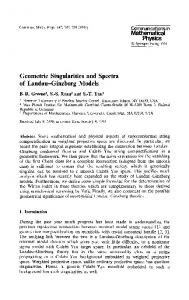
Fig. 1. Points (yj,Uj) of the Poisson process (marked by •) correspond to high local maxima of the Gaussian curve ξ(x). Critical parabolas define discontinuity points and zeros of the limit velocity process v(t,x). Then, our main result can be formulated as follows. Theorem 2.1. Let u(t, x) be the solution (1.2) of the Burgers' equation (1.1) with the initial datum ξ(x) = £z,(x), x G R, of the form (2.1) and satisfying conditions (2.3) and (2.4). Then, as L —• oo, the finite dimensional distributions of u(L2t,L2x),(t,x) G R+ x R, tend to the corresponding distributions of the random

field

v(t,x) =

yj*{t,x)

(2.5)

Here, yj*(t,x) Ξ yj* is the abscissa of the point of a Poisson process (yj,Uj)jez K2, with intensity e~ududy, which maximizes Uj — (x — yj)2/It, i.e. (χ-yr)2 it

it

on

(2.6)

The intuitive meaning of Theorem 2.1 can be best explained with the help of the geometric construction presented on Fig. 1 which, actually, goes back to the original Burgers' (1974) work. Also, notice that the limit random field v(t,x) does not depend on the viscosity parameter μ in Eq. (1.1), and that its shape is what one usually sees in the study of the Burgers' equation in the zero viscosity limit.


213

Proof of Theorem 2.1. To simplify the notation, we shall consider only the convergence of one-dimensional distributions of u(L2t,L2x) forμ = t= 1/2, x = 0. Afterwards, we shall explain how the general case can be obtained. Put HL :=u(L2 (2.7) (2.8)

1ogI where c\ = log(v^2/2π). According to (1.2), (2.1), -2fyQχv[L2(ηL(y)-y2)]dy H

where tfLiy) —aL {j\{Ly) — ^L)

(2.10)

lL

Let yj \uj = ηUyf^) be positions and heights of local maxima of the process ^(x),x G R, respectively. Due to condition (2.4) of the theorem, their number is a.s. finite on any finite interval (see Leadbetter et al. (1983), Sect. 7.6). Let (yfj-\ujlύ) be the pair which maximizes ufύ - (yfL))2 = ηL(yfL)) - {y^f, j € Z, i.e.,

(In the case when the last maximum is achieved at several points, we chose the one with the smallest ordinate.) Now, put I(A^)

= J exp [L\ηL(y) - y2)] dy,

(2.12)

where

z l ^ = [y e R : \y - y(f\ < l/LaL] .

(2.13)

Then, HL of (2.9) can be written as HL = -2where y exp [L2(ηL(y) - y2)] dy / I(ΔJ*L))

RL =

J

QL=

S exp [L2(ηL(y) - / ) ] dy / I{Δf])

, ,

(2.14) (2.15)

7*

and PL=

J (y-y^L))^v[L2(ηdy)-y2)]dy/i(A^)).

(2.16)

214


Clearly, the convergence in distribution HL => v{\/2, 0) = -2yr

,

(2.17)

follows from the facts that yfL)

^ y

Ξ ^*

r

( 1 A 0

),

(2.18)

,

(2.19)

QL => 0 ,

(2.20)

RL=>0

and from the trivial bound \pL\ < 2/LaL —• 0(L —» oo). Proof of the theorem requires a study of the Poisson convergence of functionals of a Gaussian trajectory near high local maxima, in the spirit of Chapter 10 of Leadbetter, Lindgren, Rootzen (1983). Moreover, to prove (2.18) we need a criterion for convergence of the point process (yj,Uj)jez in a topology matched to the Burgers' equation. That topology will be introduced and studied in Sect. 4. The proof of Theorem 2.1 will then be completed in Sect. 5.

3. Poisson Convergence of Local Maxima Let Jt be the space of all locally finite point measures on R 2 , with the topology of vague convergence of measures, denoted by —> (see Kallenberg (1983)). Introduce also the space Jί of all locally finite point measures on R 2 , taking values in the Banach space C[—1,1] of continuous functions, equipped with the supremum norm. || ||. Elements v G Jί can be identified with countable sequences v = (yj,uj,gj)Jez ,

(3.1)

where (yj,uj) G R 2 and gj G C [ - l , 1], j G Z. Write v = (yj,Uj)jez. Then v can be identified with the element V £ δ^yj,Uj) G Jί. The convergence vL —> v (vi, v G Jί) is equivalent to the condition that VL —> v (in Jί) and that \\9j\L-9j\\ ->0

(3.2)

for any j G Z. It is clear that Jί, as well as Jί, are complete, metrizable spaces with respect to the above topology. Without any risk of misunderstanding, we will use the same notation => for the weak convergence of random elements from Jί, Jί, and/or from a finite dimensional Euclidean space. With the Gaussian process r\ι{x) of (2.10) we associate the point process v ^ = (yfL\uJL^)jez £ Jί of local maxima, and the point process γWL) — (y^ L ^

U

^L

^g^L ^

z

£j ι^

(3.3)

which includes the "germs" g^L\ ) G C[—1,1] of the trajectory near local maxima, where, for y G [—1,1],

gJL\y) = ηL(yfL) + y/LaL) -

ηL(yfύ)

'"') + y/LaL)-u^).

(3.4)


215

Proposition 3.1. The point process vto)=>v, where v = (yj,Uj,gj)jez, with v = (yj,uj)jez 2.1, and

(3.5)

being the Poisson process of Theorem ^

^

hU]

(3.6)

being a deterministic parabola. Proof. The lemma is equivalent to the statement that both viηL)

=> v ,

(3.7)

and P - lim | | ^ } - g\\ = 0 ,

(3.8)

for any j G Z such that the corresponding local maximum (yj \uj χ

) lies in a

2

fixed compact set [xi,%2] [^1,^2] C R for all, sufficiently large L. Relation (3.7) is well-known, see e.g. Leadbetter, Lindgren, Rootzen (1983), Theorem 9.5.2. Statement (3.8) can be proved using the Slepian model process representation near a local maximum (due to Lindgren (1970)) as follows. In view of the above, it suffices to prove that, for any ε > 0, ΣP \\\Q{jL) -g\\>ε,

(y^Kuf^)

e [χi,*2] x [uuu2]] - o ,

(3.9)

as L —> oo. Write the left-hand side as

[[P [\\g ^-g\\ > ε\yf ,u^] (

ύ

• 1 ( o ^ , ^ ) 6 [xuxi] x [uuu2] (3.10)

According to Theorem 3 of Lindgren (1970),

2

\λ2x \

^

> εl , 1

(3.11)

where vι = aι + (u + c\~)jaιand, for any u 6 R , η"(x) = vA(x) + ζ,(x) - ζ2,B(x),

x e [-1,1] ,

is the Slepian model process conditioned at a local maximum of height v at x = 0. Here A(x) = (λ4r(x) + λ2r"(x))/D, D = λ4 - λ\ > 0, while d(jc) and ζ2,Ό(x) are independent stochastic processes with

where B(x) = (A2r(x) + r (x))/D, and κ:y > 0 is a random variable with the density proportional to zexp[—(z — λ2v)2/2D],z > 0. The process ζ\(x) is a zero mean Gaussian process with the covariance function C(x,y) given in Lindgren (1970),

216


Eq. (8). Making use of condition (2.4), and the fact that A(0) = 1, Af(0) = A"(0) = 0, one easily obtains that aLvL(A(x/aL) - I) ^ 0 , uniformly in x e [—1, l],u e [uuu2]. Next, using the fact that ζ\(x) is a.s. continuously differentiable, and that ζ\(0) = ζ\(0) — 0, similarly as in Leadbetter, Lindgren, Rootzen (1983), p. 203, we conclude that sup aL\ζι(x/aL)\ -^ 0,

a.s .

Finally, noting that sup -aLvLλ2B(x/aL)+-λ2x and denoting by pLfU

0,

2

the probability in (3.11), we obtain that > ε] + o ( l ) - > 0 ,

PL,« = P[\l - (κΌL/λ2vL)\

(3.12)

uniformly in u£[u\,u2], as κv/λ2v —» 1 (v —»oo), in probability. Since (yfL\uJlL))jez = v{ηL) converges to a Poisson limit (see (3.7)), relations (3.10)(3.12) imply (3.8) and the proposition itself. QED Proposition 3.1 immediately yields the following lower bound for the exponential integral in (2.12). Corollary 3.1. For any compact A c R2, and any ε, δ > 0, there exists an Lo < oo such that, for every L > LQ, ( ) J

αo, β > βo,

< oo.

(4.3)


217

Proof. The lemma follows easily from the well-known properties of Jί and of the vague topology (Kallenberg (1983), 15.7), and from the following observation. Let vι —> v and sup£(/α/β/(vz,) + / α " #/(VL)) < oo for some αo < 0 f° r z'4=7 It follows from (2.5) that both the distribution of (6.1), and its joint moment (ft-point correlation function) p^n\t\,x\,...,tn,xn) = Eυ(t\,x\)...v(tn,xn), can be obtained from the distribution P*(-;(t,x)n)=P[(y*)ne']

(6.2)

(y*)n = (y*,...,y*n),

(6.3)

of the random vector where y* = yj? = yrc*,*) > / = 1,...,«, and we use the notation ( Λ = (^i (t,χ)n

Λ)eR",

= ((tι,χλ),...9(tn,xn))

e ( R + x R)n .

In particular,

p^(t,x)n

= / ft X~^P* (d(y)nl (t,x)n) . n ,=1

R

(6.4)

'

We have ()

( '(^)«)'

(6 5 )

where the sum is taken over all partitions (A)m = (A\,...,Am) of {1,...,«},^4/ Φ0, ^ n ^ = 0 ( i + y ) , U ^ , 4 = { l , . . . , « } , m = l , . . . , « , a n d ^ ^ ^ j ^ α x ^ ) is a measure on R w which can be identified with the distribution of (y*)n on the mdimensional hyperplane y* = yk,

i^Λk,

A=l,...,m.

(6.6)

Note that the last event occurs if, and only if, for every k = l , . . . , m , and any Poisson point (yj9Uj),jΦk, the following inequality is true: W/ < Λ feOy) ,

(6.7)

where te(7) = uk + —((y-xtf

- (yk -Xi)2)

(6.8)

is the parabola passing through the point (yk,Uk) and "centered" at xi9i G ^ . Using the well-known formula for the Poisson probabilities, we obtain from (6.7) that for


224

each partition (A)m, the measure P^m( l(t9x)n) is absolutely continuous in R m , and that the corresponding Radon-Nikodym density is given by

-Σ««-/V V
*2 = — : —, (6.13) h -t\ t 2 - t\ or x\/t\ —χ2lh. Substituting (6.13) into (6.11) and (6.12), after some elementary, but tedious, transformations we arrive at the formula 1

p

(ti,x\',t2,x2)

oo

= — J (z — x\)(z — x2)A~ hh-oo

(z;x2,x2)dz

" / l z i(l ~ hh -oo where

/

\y\\z\

The corresponding expression for fixed time {t\ — t2 = t) covariance was obtained in Gurbatov, Malachov, Saichev (1991) p. 181, and is somewhat simpler, namely p{2Xt,xι\t9x2)=~{ t dx where P,(2x) = (1/v^πO / [e(x+z)

l2t

Φt{x+z)

+ e{x~z)

/2

'Φt(x -

with, as usual, Φt(x) = (l/V2πt) /f.^ e u l2tdu, being the probability that the points x\9 x2, x2 - x\ = 2x9 belong to the same line segment of continuity of the sawtooth process v(t9x) (see Gurbatov, Malachov, Saichev (1991), pp. 175-181, for details).

References 1. Albeverio, S., Molchanov, S.A., Surgailis, D.: Stratified structure of the Universe and Burgers' equation: A probabilistic approach. Prob. Theory Rel. Fields (1995), to appear 2. Bulinskii, A.V., Molchanov, S.A.: Asymptotic Gaussianness of solutions of the Burgers' equation with random initial data. Teorya Veroyat. Prim. 36, 271-235 (1991) 3. Burgers, J.: The Nonlinear Diffusion Equation. Amsterdam: Dordrecht (1974) 4. Chorin, A.J.: Lectures on Turbulence Theory. Berkeley CA: Publish or Perish (1975) 5. Fournier, J.-D., Frisch, U.: L'equation de Burgers deterministe et statistique. J. Mec. Theor. Appl. 2, 699-750 (1983) 6. Funaki, T., Surgailis, D., Woyczynski, W.A.: Gibbs-Cox random fields and Burgers' turbulence. Ann. Applied Probability 5, to appear (1995) 7. Gurbatov, S., Malakhov, A., Saichev, A.: Nonlinear Random Waves and Turbulence in Nondispersive Media: Waves, Rays and Particles. Manchester: Manchester University Press (1991) 8. Hopf, E.: The partial differential equation ut + uux = μuXλ. Comm. Pure Appl. Math. 3, 201 (1950)

226


9. Hu, Y., Woyczynski, W.A.: An extremal rearrangement property of statistical solutions of the Burgers' equation, Ann. Applied Probability 4, 838-858 (1994) 10. Kallenberg, O.: Random Measures. New York: Academic Press (1983) 11. Kraichnan, R.H.: Lagrangian-history statistical theory for Burgers' equation. Physics of Fluids 11, 265-277 (1968) 12. Kraichnan, R.H.: The structure of isotropic turbulence at very high Reynolds numbers. J. Fluid Mech. 5, 497-543 (1959) 13. Kwapien, S., Woyczynski, W.A.: Random Series and Stochastic Integrals: Single and Multiple, Boston: Birkhauser (1992) 14. Leadbetter, M.R., Lindgren, G., Rootzen H.: Extremes and Related Properties of Random Sequences and Processes. Berlin, Heidelberg, New York: Springer (1983) 15. Lindgren, G.: Some properties of a normal process mear a local maximum. Ann. Math. Stat. 41, 1870-1883 (1970) 16. Rice S.O.: Mathematical analysis of random noise. Bell System Tech. J. 24, 46-156 (1945) 17. Shandarin, S.F., Zeldovich, Ya.B.: Turbulence, intermittency, structures in a self-gravitating medium: The large scale structure of the Universe. Rev. Modern Phys. 61, 185-220 (1989) 18. Sinai, Ya.G.: Two results concerning asymptotic behavior of solutions of the Burgers equation with force. J. Stat. Phys. 64, 1-12 (1992) 19. Sinai, Ya.G.: Statistics of shocks in solutions of inviscid Burgers' equation. Commun. Math. Phys. 148, 601-621 (1992) 20. Surgailis, D., Woyczynski, W.A.: Scaling limits of solutions of the Burgers' equation with singular Gaussian initial data, in Chaos Expansions, Multiple Wiener-Ito Integrals and Their Applications, C. Houdre and V. Perez-Abreu, Eds, pp. 145-161, Boca Raton, Ann Arbor CRC Press (1994) 21. Woyczynski, W.A.: Stochastic Burgers' Flows. In: Nonlinear Waves and Weak Turbulence. Boston: Birkhauser, pp. 279-311 (1993) Communicated by Ya.G. Sinai