Mathematical Principles of Fuzzy Logic

Mathematical Principles of Fuzzy Logic

MATHEMATICAL PRINCIPLES OF FUZZY LOGIC

´ NOVAK ´ VILEM University of Ostrava Institute for Research and Applications of Fuzzy Modeling Brafova 7, 701 03 Ostrava 1, Czech Republic

IRINA PERFILIEVA Moscow State Academy of Instrument Making Stromynka 20, 107846 Moscow, Russia and University of Ostrava Institute for Research and Applications of Fuzzy Modeling Brafova 7, 701 03 Ostrava 1, Czech Republic

ˇÍ MOCKO ˇ R ˇ JIR University of Ostrava Institute for Research and Applications of Fuzzy Modeling Brafova 7, 701 03 Ostrava 1, Czech Republic

Kluwer Academic Publishers Boston/Dordrecht/London

To David and Martin, to Vitalij, to Soˇ na, Marek and Kateˇrina, with love

Contents

List of Figures

ix

List of Tables

xi

Preface

xiii

1. FUZZY LOGIC: WHAT, WHY, FOR WHICH? 1.1 Vagueness and Uncertainty 1.2 Vagueness and Fuzzy Sets 1.3 What Is Fuzzy Logic 1.4 Outline of the Agenda of Fuzzy Logic

1 2 6 9 12

2. ALGEBRAIC STRUCTURES FOR LOGICAL CALCULI 2.1 Algebras for Logics 2.1.1 Boolean algebras 2.1.2 Residuated lattices and MV-algebras 2.2 Filters and Representation Theorems 2.3 Elements of the theory of t-norms 2.4 Introduction to Topos Theory 2.4.1 Topos theory 2.4.2 Lattice of subobjects in topos

15 16 16 23 35 41 52 52 56

3. LOGICAL CALCULI AND MODEL THEORY 3.1 Classical Logic 3.1.1 Propositional logic 3.1.2 Predicate logic 3.1.3 Many-sorted predicate logic 3.2 Classical Model Theory 3.3 Formal Logical Systems 3.4 Model Theory in Categories

61 61 62 67 73 73 77 82

4. FUZZY LOGIC IN NARROW SENSE 4.1 Graded Formal Logical Systems 4.2 Truth Values 4.2.1 Intuition on truth values and operations with them 4.2.2 Truth values as algebras 4.2.3 Why Lukasiewicz algebra

93 95 104 104 109 110

v

vi


4.3

4.4

4.5

4.6

4.2.4 Enriching structure of truth values Predicate Fuzzy Logic of First-Order 4.3.1 Syntax and semantics 4.3.2 Basic properties of fuzzy theories 4.3.3 Consistency of fuzzy theories 4.3.4 Extension of fuzzy theories 4.3.5 Henkin fuzzy theories 4.3.6 Complete fuzzy theories 4.3.7 Lindenbaum algebra of formulas and its properties 4.3.8 Completeness theorems 4.3.9 Sorites fuzzy theories 4.3.10 Partial inconsistency and the consistency threshold 4.3.11 Additional connectives 4.3.12 Disposing irrational logical constants Fuzzy Theories with Equality and Open Fuzzy Theories 4.4.1 Fuzzy theories with equality 4.4.2 Consistency theorem in fuzzy logic 4.4.3 Herbrand theorem in fuzzy logic Model Theory in Fuzzy Logic 4.5.1 Basic concepts of fuzzy model theory 4.5.2 Chains of models 4.5.3 Ultraproduct theorem Recursive Properties of Fuzzy Theories

111 112 113 118 127 129 136 137 140 145 147 148 150 152 156 156 157 163 165 165 169 170 173

5. FUNCTIONAL SYSTEMS IN FUZZY LOGIC THEORIES 5.1 Fuzzy Logic Functions and Their Representation by Formulas 5.1.1 Formulas and their relation to fuzzy logic functions 5.1.2 Piecewise linear functions and their representation by formulas 5.2 Normal Forms for FL-Functions and Formulas of Propositional Fuzzy Logic 5.2.1 Normal forms for L-valued FL-functions 5.2.2 Normal forms for functions represented by formulas 5.3 FL-Relations and Their Connection with Formulas of Predicate Fuzzy Logic 5.3.1 FL-Relations and Their Representation by Formulas 5.3.2 Normal Forms and Approximation Theorems 5.3.3 Representation of FL-relations and Consistency of Fuzzy Theories 5.4 Approximation of Continuous Functions by Fuzzy Logic Normal Forms 5.4.1 Approximation of continuous functions by FL- relations 5.4.2 Approximation of continuous functions determined by a defuzzification operation 5.5 Representation of Continuous Functions by the Conjunctive Normal Form

177 179 179 183 187 188 193 198 199 201 206 208 208

6. FUZZY LOGIC IN BROADER SENSE 6.1 Partial Formalization of Natural Language 6.1.1 Evaluating and simple conditional linguistic syntagms 6.1.2 Translation of evaluating syntagms and predications into fuzzy logic 6.1.3 The meaning of simple evaluating syntagms 6.2 Formal Scheme of FLb 6.3 Special Theories in FLb 6.3.1 Independence of formulas

221 222 222 225 229 237 240 240

211 216

Contents

6.3.2 6.3.3

Deduction on simple linguistic descriptions Fuzzy approximation based on simple linguistic descriptions

vii 245 247

7. TOPOI AND CATEGORIES OF FUZZY SETS 7.1 Category of Ω-sets as generalization of fuzzy sets 7.2 Category of Ω-fuzzy sets 7.2.1 Ω-fuzzy sets over MV-algebras 7.3 Interpretation of formulas in the category CΩ − Set

257 259 274 275 289

8. FEW HISTORICAL AND CONCLUDING REMARKS

301

Appendices

306

A– Brief overview of some selected concepts

307

References

309

List of Figures

1.1 1.2 6.1

Membership function of the fuzzy set of “small numbers”. Possible forms of the fuzzy sets assigned as the meaning to the basic syntagms “small”, “medium age”, “old” from T (Age). Typical membership functions of simple evaluating syntagms.

7 13 231

ix

List of Tables

xi

Preface

This book is an attempt to provide a systematic course of the formal theory of fuzzy logic. We made a lot of effort to be precise, but at the same time to explain the motivation and interpretation of all the results and, if possible, to accompany the theory by examples. There are a lot of other books on various aspects of fuzzy logic. Our book is more specific from the point of view of several aspects. First, it is based on logical formalism demonstrating that fuzzy logic is a well developed logical theory. Second, it includes the theory of functional systems in fuzzy logic, which provide explanation of what, and how can be represented by formulas of fuzzy logic calculi. Third, except for the generalization of the classical way of interpretation within the environment of fuzzy sets constructed over classical sets, it also presents much more general interpretation of fuzzy logic within the environment of other proper categories of fuzzy sets stemming either from the topos theory, or even generalizing the latter. Last but not least, the leading philosophical point of view is presentation of fuzzy logic especially as the theory of vagueness as well as the theory of the common-sense human reasoning, which is based on the use of natural language, the distinguished feature of which is vagueness of its semantics. We expect the book to be read by people interested in fuzzy logic and related areas, and also by logicians, mathematicians and computer scientists interested in mathematical aspects of fuzzy logic. It can be used in special courses of fuzzy logic, artificial and computational intelligence, in master and post-gradual university studies, in advanced courses on various applications including fuzzy control, decision-making and others. The book is divided into eight chapters. The first chapter is introductory and it provides motivation for the development of fuzzy logic, describes its structure and outlines its potential for applications. Fuzzy logic is there divided into that in narrow sense (FLn), which is a special many-valued logic aiming at description of the vagueness phenomenon and that in broader sense (FLb), whose aim is to provide a formal theory for modeling of natural human deduction based on the use of natural language. It is argued that characterization of the vagueness phenomenon is fundamental for further development of fuzzy logic as well as its applications. xiii

xiv


The second chapter is an overview of the basic algebraic concepts necessary for characterization of the structure of truth values and for understanding to the subsequent chapters. The third chapter briefly reminds basic concepts of classical logic, and also the notation which is employed further. The main chapters of the book are fourth to seventh. The fourth chapter contains explanation of fuzzy logic in narrow sense. We confine ourselves mainly to fuzzy logic based on the Lukasiewicz algebra of the truth values. Many reasons have been given arguing that this requirement is a necessary consequence of the assumptions, which seem to be natural and convincing. Among them, essential are continuity of the connectives (this follows from the conviction that vagueness phenomenon requires continuity) and completeness (balance between syntax and semantics). We prove lemmas and theorems characterizing behaviour of FLn, including deduction, contradiction, and others. The main result is the completeness theorem. Besides this, we also outline fundamentals of the model theory and discuss questions concerning computability. The fifth chapter describes functional systems related to propositional and predicate calculi of fuzzy logic. A notable role here is played by the well known McNaughton theorem. We provide a constructive proof of it and then, deduce a canonical representation of formulas of propositional fuzzy logic as well as some special representation of formulas of predicate fuzzy logic. A special attention has been paid to the generalization of disjunctive and conjunctive normal forms into fuzzy logic. Among the main properties of them, the ability to represent approximately continuous functions including evaluation of the quality of the approximation has been investigated. The sixth chapter extends the previous theory to obtain a theory of parts of natural language to constitute fuzzy logic in broader sense. We present a formalization of the concepts of intension and extension, evaluating linguistic syntagms and linguistic description (a set of IF-THEN rules), and demonstrate some theorems characterizing their behaviour. The seventh chapter is more abstract and deals with fuzzy sets and fuzzy logic within category theory. First, we present properties of three possible categories of fuzzy sets. The subsequent sections provide the reader with a general picture of fuzzy logic interpreted in topos and its place in topos logic. We tried to show two possible approaches. The first one is based on topos theory and Heyting algebra structures defined on the set of subobjects. The second one is based on the MV-algebra structures defined on these sets. In this book, we present some of the results and consequences, which could be useful from the point of view of fuzzy set theory. In particular, we tried to show explicitly similarities between the obtained categories and topoi, and to show how the internal logic in these categories could be directly developed. The book is concluded by a short, eighth chapter giving a brief overview of the history of fuzzy logic and outlining some of its actual problems to be solved in the future. Sections 2.4, 3.4 and Chapter 7 have been written by J. Moˇckoˇr. Chapter 5 has been written by I. Perfilieva and Chapters 4 and 6 by V. Novák. The rest has has been written by by the latter two authors together.

PREFACE

xv

This book has been prepared mostly in the Institute for Research and Applications of Fuzzy Modeling of the University of Ostrava, Czech Republic, which has been established on the basis of the project VS 96037 of the Ministry of Education, Youth and Physical Training of the Czech Republic. Some parts have been prepared also in the Moscow State Academy of Instrument-Making and Informatics, Russia, and Institute of the Theory of Information and Automation of the Academy of Sciences of the Czech Republic. We wish to express our thanks to all who helped us in the preparation of this book. On the first place, we thank to people whose work has been for us the ˇ main source of knowledge and inspiration, namely P. Hájek from UI AS CR, U. H¨ ohle from the University of Wuppertal, D. Mundici form the University of Milano and A. diNola from the University of Salerno. Further, we thank to the people who have read the manuscript and helped us to improve it on many places, namely to R. Bˇelohlávek and A. Dvoˇrák from IRAFM, University of Ostrava, and to S. Gottwald from the University of Leipzig. We want also to thank to our Chinese friends, M. Ying and G. Chen from Beijing Tschingua University, and G. Wang from ShaanXi Normal University for their hospitality, which helped to write some parts of this book during the stay of the first two authors in China. Last but not least, we want to thank to Prof. T. Kreck, director of the Institut f¨ ur Mathematik in Oberwolfach, and also to other workers of it for providing us unexceptionable working conditions in which significant portions of the book have been written.

Ostrava, May 1999 Vilém Novák, Irina Perfilieva, Jiˇr´ı Moˇckoˇr

1

FUZZY LOGIC: WHAT, WHY, FOR WHICH?

The discussion about the philosophical background and the role of fuzzy logic in science has not been finished till now. Since this book focusses on the mathematical principles of fuzzy logic, it is necessary to explain our point of view on the questions and concepts which led to it. Our aim is to demonstrate the reader that the key role in the roots of fuzzy logic is played by the vagueness phenomenon, which gives rise to problems not addressed by classical logic, but which are important to solve. For this purpose, we divided the chapter as follows. In Section 1.1, we analyze two complementary phenomena, namely uncertainty and vagueness. A detailed discussion of both of them should reveal the reader that fuzzy logic deals with the latter while probability and few other theories1 deal with the former. Section 1.2 continues discussion on vagueness and demonstrates the way how it is captured by fuzzy set theory, which is unseparably joined with fuzzy logic. Sections 1.3 and 1.4 give answer to the questions, what is fuzzy logic, what is its agenda and what is it useful for. Fuzzy set theory as well as fuzzy logic originated from ideas of Lotfi A. Zadeh. His seminal paper [ 136] published in 1965 contains the concept of fuzzy set and establishes basic principles of its theory. The most elaborated form of the basic idea of fuzzy logic can be found in [ 140, 141].

1 In

connection with fuzzy logic, one may meet, for example, the possibility theory. As will be seen, this addresses uncertainty rather than vagueness.

1

2


1.1

Vagueness and Uncertainty

The discussion in this section focuses on two phenomena whose importance in science raised especially in this century, namely uncertainty and vagueness. Both these concepts characterize situations in which we regard2 phenomena surrounding us; they are concerned with the amount of knowledge we have at disposal (or can have at disposal), which, however, is limited (mostly in principle). Our main goal is to show that these phenomena are two, rather complementary facets of a more general phenomenon which we will call indeterminacy 3 . Uncertainty. This phenomenon4 emerges due to the lack of knowledge about the occurrence of some event. It is encountered when an experiment (process, test, etc.) is to proceed, the result of which is not known to us. Let us stress that there is no uncertainty after the experiment was realized and the result is known to us. Note that the word “occurrence” inherently involves time, i.e. uncertainty is always connected with the question whether the given event may be regarded within some time period, or not. This becomes apparent on the typical example with tossing a player’s cube. The phenomenon to occur is the number of dots on the cube and it occurs after the experiment (i.e. tossing the cube one times) has been realized. A specific form of uncertainty is randomness. This has first been touched in science by the probability theory which has been founded by Jakob Bernoulli (1654-1705). He himself has not abandoned the deterministic point of view and took his theory as an attempt to characterize our expectation of the process of occurring phenomena in the world. Randomness was considered to raise mainly due to extensive number of outer influences causing ambiguity in the result, thus preventing us to describe it as deterministic. As late as in the 20th century, mainly in connection with important discoveries in atomic physics and quantum mechanics, randomness had been recognized to be unavoidable and a deep feature of the nature. In quantum mechanics , the concept of randomness is fundamental since the theory provides only the probability of results. As already outlined, the mathematical model (i.e. quantified characterization) of the uncertainty phenomenon is provided especially by the probability theory. In everyday terminology, probability can be thought of as a numerical measure of the likelihood that a particular event will occur. Recall that the 2 By

“regarding” we mean learning the world in the most general way, i.e. by senses as well as by reason. 3 We have chosen the term “indeterminacy” to encompass both phenomena discussed below, namely uncertainty as well as vagueness. This term, in the meaning very close to ours, can be found also in other sources, for example in Merriam Webster or Encyclopedia Brittanica. Note that in the literature, for example on fuzzy set theory, one may meet the term “uncertainty” in our meaning of “indeterminacy”. 4 The concept of “phenomenon” is left unexplained and taken as primitive. We suppose that the reader has some idea of what phenomenon is and we will better give some examples than attempt at providing a kind of exhausting philosophical explanation which, all in all, still might turn out to be unsatisfactory.


3

probability values are taken from the scale [0, 1] where values near 1 indicate that an event is likely to occur while those near 0 indicate the opposite. The probability of 0.5 means that an event is equally likely to occur as well as not to occur. There are also other mathematical theories addressing the uncertainty phenomenon, for example the possibility theory, belief measures and others. Vagueness. This phenomenon raises during the process of grouping together objects5 having some property ϕ (of objects). Its result will be called a grouping of objects. In a slightly formal way, the grouping can be written as X = {x | x has the property ϕ}

(1.1)

where x varies over objects. It is important to stress that, in general, the grouping X cannot be taken as a set since the property ϕ may not make us possible to characterize the grouping X precisely and unambiguously; there can exist borderline elements x for which it is unclear whether they have the property ϕ (and thus belong to X), or not. For example, is it possible to imagine “all tall people”, “all beautiful flowers on the meadow”, “all witty novels”, etc? These are typical examples of vaguely formed groupings of objects put together using, sometimes extremely complicated, property (try to define “beautiful flower”!). On the other hand, it is always possible to characterize, at least some typical objects, i.e. objects having typically the property in concern. For example, everybody can show a “blue sweater” or “huge building” but it is impossible to show “all huge buildings”. The objects, which can be unambiguously decided to have ϕ, will be called prototypes. In general, we say that X, which is delineated using a property enabling borderline cases, has unsharp boundaries. The following example will often be brought back in the sequel. Example 1.1 A typical vague property is to be a small natural number. Can we imagine all the small natural numbers? Clearly, 0 is small, 1 is small as well, etc. But where does this sequence finish? The only sure fact is that there exists a number, say 1, 000, 000, 000, which is not small. An attempt at sharp (exact) explanation would mean to be able to find a small natural number n, 0 < n < 1, 000, 000, 000 such that n + 1 is not small. However, such a conclusion can hardly be defended. If n is small then n+1 must 5 The

concepts of object and property are also taken as primitive. P. Vopˇ enka in [ 130] provides the following characterization. An object is a phenomenon which we separate in the world, i.e. a phenomenon to which we concede its individuality making it distinct from the other phenomena. Objects are usually accompanied by other kind of phenomena called properties. The same property may be applicable to more than one object. Thus, for example, a “pen” is an object accompanied by the properties “to be blue, narrow, fine”, etc., but we may also have “blue flowers”, “blue ink”, “blue eyes”, etc. It is natural for the human mind to construe as objects so much phenomena as possible. Thus, properties may be also often viewed as objects (cf., for example, “roundness, colour, length”, etc.).

4


be small, as well. Hence, there is no last small number before 1, 000, 000, 000 and no first number n < 1, 000, 000, 000 which is not small. We can distinguish small numbers from big ones but we are not able to say unambiguously about each number whether it is small or not. The property of “small” is vague and small numbers disappear inside the sequence of numbers ranging from 0 to 1,000,000,000. Consequently, they form a vague grouping of numbers. 2 Vagueness has not been investigated so long as uncertainty. The interest in it appeared in science as late as in this century. One of the first philosophical papers about it has been published by B. Russell in 1923 (see [ 117]). Another important one [ 10] was written by M. Black 14 years later. However, the real interest came only after the fuzzy set theory had been founded. Let us stress that vagueness stems from the way how people regard the world and phenomena in it. Our mind forms concepts via some kind of “idealization” process. However, the nature itself is only in a partial coincidence with such idealization and namely, there is no vagueness in the nature. Vagueness is an opposite to exactness and we argue that it cannot be avoided in the human way of regarding the world. Any attempt to explain an extensive detailed description necessarily leads to using vague concepts since precise description contains abundant number of details. To understand it, we must group them together — and this can hardly be done precisely. It is likely that the explanation would significantly rely on the use of natural language since vagueness is often connected with its use. However, the problem lays deeper, in the way how people regard the phenomena around them. We may thus conclude that the increase of exactness leads to an increase in the amount of information whose relevancy then decreases until a point is reached after which the preciseness and relevancy are mutually excluding characteristics. This is the famous incompatibility principle described by L. A. Zadeh in [ 139]. It demonstrates that vagueness is necessary to convey relevant information. Vagueness should be distinguished from generality and from ambiguity. In our terms, to be more general means to take into account more (various) groupings of objects, while ambiguity occurs in the language when more alternative meanings are assigned to the same word expression. For example, “colour” is more general than “red”, since the former concerns various groupings of objects being red, green, etc. and each concrete colour represents a vague property. Continuity of vagueness. A typical feature of vagueness is its continuity. This means that if an object has a vague property and another one differs very little from it, then it must have the same property. In other words, a small difference between objects cannot lead to abrupt change in the decision of whether either of them has, or has not a vague property. The transition from having a (vague) property to not having it is smooth. As an example, let us recall from [ 10] the “museum of applied logic” consisting of a series of “chairs”. It begins with a typical chair and ends up with a lump of wood apparently not being a chair. Each two neighbouring chairs in the series differ by some small piece cut from one of them. But since this piece


5

can be arbitrarily small, there are no two neighbouring members in this series such that one is a chair and the second one is not. Consequently, the meaning of “chair” is vague and the transition from chair to non-chair is continuous. Let us stress that the continuity feature of the vagueness phenomenon will play an important role throughout this book. A mathematical theory of the vagueness phenomenon is most successfully provided by fuzzy logic. Another deep mathematical theory addressing, among others, also vagueness is the Alternative Set Theory (AST) (see [ 129, 130] and possibly also [ 89]). Comparison of uncertainty and vagueness. Let us now compare both discussed phenomena, which, as noted above, are two facets of the indeterminacy. It is principal for the uncertainty that occurrence of some phenomenon (one of many ones) is a result of an experiment. The substance of the former is irrelevant. More phenomena may occur, but we have not enough knowledge to determine, which one. The situation may thus be characterized as a classification of one result to fall into some of many classes. Vagueness concerns the way how the phenomenon itself is delineated and disregards whether it occurs or not. The phenomenon is represented by “one” unsharp grouping of “many” objects. Hence, we may briefly say that vagueness raises as many-to-one relation while uncertainty raises as one-to-many. It has to be stressed that in the reality, we encounter indeterminacy with both its facets present. The difference between vagueness and uncertainty may also be characterized from another side on the basis of the conflict between actuality and potentiality as discussed in the set theory. In classical set theory, every set is understood to be actualized, i.e. we imagine all its elements to be already existing and at disposal to us in one moment. This concerns both finite as well as infinite sets. Though we can always see only part of the infinite set, our reasoning about any set stems from the assumption that it is at our disposal as a whole. On the other hand, most events around us are only potential, i.e. they may, but need not, to occur or happen. Thence, the difference between actuality and potentiality corresponds to the difference between vagueness and uncertainty. Vagueness stems from the actualized non-sharply delineated groupings while uncertainty is encountered when dealing with still non- actualized ranges of objects. The latter means that we may speculate about the range X, but only part of it indeed exists. Furthermore, once an actualized (i.e. already existing) grouping of objects from the range X is at our disposal, it has sense to speak only about the truth of the fact that some element belongs to it. Indeed, let an object y we are thinking of be created. If we learn that it has a property ϕ (cf. (1.1)), we know that it falls into X 6 , i.e. we know that it is true that y ∈ X. However, in general it is uncertain whether y will be created (will exist) or not and thus, we cannot speak about the truth of y ∈ X.

6 More

precisely, it falls into the existing part of X.

6


1.2

Vagueness and Fuzzy Sets

In the previous section, we have widely discussed the vagueness phenomenon, which for a long time has been neglected by the European science. “Blackand-white” reasoning is apparent especially in mathematics: either the fact holds, or it does not, and nothing else. In science, we cannot avoid this way of thinking as any kind of releasing from it led to serious mistakes in the past. On the other hand, strictly two-valued thinking brings us nearer to the world of Platon than to the common-day-to-day life. The latter is not so simple. There are no purely good or purely bad people; if few drops fall down then it is difficult to say whether it rains; and even white snow is often a little black (especially in industrial towns). Vagueness is hidden in the way how people regard phenomena surrounding them. Mathematics faces the problem, how vague groupings of objects can be characterized. Classical set theory does not carry any vagueness since there was no interest in it. Fuzzy set theory is an attempt to find such an approximation of vague groupings which in situations where, for example, natural language plays a significant role, would be more convenient than classical set theory. Graded approach. Throughout this book, we will follow a very general principle, which we will call the graded approach, or as a kind of jargon, the fuzzy approach. This means the use of a scale when characterizing a relation between object and its property. The graded approach seems to be a general principle of the human mind, which uses it when trying to specify whether the object possesses the property fully or only partly, though the given property is vague. For example, we often say “almost white dress”, “very strong engine”, “too unpleasant situation”, etc. In all these examples, we may encounter hidden degrees of intensity of the property in concern. The graded approach will be mathematized by means of a special scale being an ordered set. In order to be sufficiently general and to be able to capture the continuity feature of vagueness, we will suppose that this set is uncountable. Furthermore, to be able to represent various manipulations with the properties partly possessed by objects, we will endow the scale by additional operations. The result is a specific algebra. There are several classes of algebras used as scales in the graded approach. They will be studied in Chapter 2. The result of the graded approach to vague groupings are fuzzy sets. We present some basic ideas of the fuzzy set theory in the next subsection. Fuzzy set theory. The decision whether the concrete object x has the property ϕ (e.g. “small”, “tall”, “light”, “blue”, etc.) is tantamount to the question whether it is true that x has it (in positive case, we will usually write ϕ(x)). However, such a question cannot be unambiguously answered. A reasonable solution consists in using some kind of a scale whose elements would express various degrees of truth of ϕ(x). Let U be a sufficiently large set from which we take the objects x. This set is called the universe. Note that this assumption is not restrictive since such a set always exists. For example, when talking about height of people (in cm),


7

we may put U = {x ∈ R | 0 ≤ x ≤ 300}. Furthermore, let L be a scale of truth values having the smallest 0 and greatest 1 elements, respectively. We usually put L = [0, 1] but this is only an unnecessary commonsense caused by the fact that this interval is very natural and transparent. Thus, 1 expresses that ϕ(x) holds (x has the property ϕ) without any doubt while 0 means that ϕ(x) does not hold at all. The other values mean that ϕ(x) holds only partly. Definition 1.1 The fuzzy set A is identified with a function A : U −→ L

(1.2)

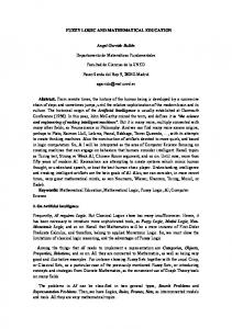
assigning a value A(x) ∈ L to each element x ∈ U . The value A(x) ∈ L is the membership degree of x in A. The function (1.2) is also called the membership function of the fuzzy set A. We will therefore use the same symbol for both and write A ⊂ U if A is a fuzzy ∼ set in the universe U . Explicitly, we will write down the fuzzy set as { A(x) x | x ∈ U } (1.3) where the couple A(x) x means “the element x belongs to A with the membership degree A(x)”, A(x) ∈ L. The value A(x) expresses the degree of truth that the element x belongs to A. 1

0.5

10

Figure 1.1.

80

150

N

Membership function of the fuzzy set of “small numbers”.

Recall Example 1.1 of the vague grouping of small numbers. In the fuzzy set theory, it can be approximated by the fuzzy set given by the (continuous) membership function depicted on Figure 1.1. In this picture, the numbers smaller than or equal to 10 are “surely small”, i.e. they are prototypes of the property “small”. Then the truth of the fact that the given number x is small diminishes until x = 150 beyond which it completely vanishes. Thus, the fuzzy set of small numbers can be written as Small(x) = { 1 0, . . . , 1 10, . . . , 0.5 80, . . . , 0.1 149}. Of course, the concrete numbers depend on the context in which we consider the property of “being a small number”. However, the course of the membership function is the same in all contexts.

8


Note that the membership function is a generalization of the characteristic function of the ordinary set. The crucial difference between the ordinary set and fuzzy set is thus in using of the scale L. Few basic concepts of fuzzy set theory. Let us now very briefly overview some basic notions of the fuzzy set theory. More details can be found in the extensive literature (see e.g.[ 22, 58, 85, 87], or from newer ones [ 57]). Let the fuzzy set A ⊂ U be given by the membership function (1.2) where ∼ L = [0, 1]. Let A, B ⊂ U . Then A ⊆ B if A(x) ≤ B(x) holds for all x ∈ U . ∼ The set of all fuzzy sets on U is F(U ) = {A | A ⊂ U } = LU . ∼ Note that F(U ) contains also all ordinary subsets of U . Given the fuzzy set A ⊂ U , it can be characterized in several ways. The ∼ following are important ordinary sets defined on the basis of A. (i) Support Supp(A) = {x | A(x) > 0},

(1.4)

(ii) a-cut Aa = {x | A(x) ≥ a},

a ∈ (0, 1],

(1.5)

(iii) Kernel Ker(A) = {x | A(x) = 1}.

(1.6)

The fuzzy set A is normal if Ker(A) 6= ∅. The empty fuzzy set is defined by ∅ = { 0 x | x ∈ U }. Obviously, this is the ordinary empty set. The basic operations with fuzzy sets are defined using their membership functions. Given fuzzy sets A, B ⊂ U . ∼ (i) Union of A and B is a fuzzy set A∪B ⊂ U with the membership function ∼ C = A ∪ B,

iff

C(x) = A(x) ∨ B(x),

x∈U

(1.7)

where ∨ denotes ‘supremum’. (ii) Intersection of A and B is a fuzzy set A ∩ B ⊂ U with the membership ∼ function C = A ∩ B,

iff

C(x) = A(x) ∧ B(x),

x∈U

(1.8)

where ∧ denotes ‘infimum’. Both union as well as intersection of two fuzzy sets may be extended to arbitrary classes of fuzzy sets provided that suprema and infima of arbitrary sets exist in L. (iii) Complement A¯ is the fuzzy set ¯ A(x) = ¬A(x) = 1 − A(x),

x ∈ U.

(1.9)


9

Note that the above definition of the basic operations with fuzzy sets is not the only possibility. The operations of infimum, supremum and negation used in equations (1.7)–(1.9) belong to more general classes of operations, which are analyzed in Section 2.3. We finish with the definition of the concept of a fuzzy relation which generalizes the classical concept of relation and which is quite often used in the sequel. Definition 1.2 Let U1 , . . . , Un be sets. An n-ary fuzzy relation R is a fuzzy set R ⊂ U1 × · · · × Un . ∼ 1.3

What Is Fuzzy Logic

The term “fuzzy logic” has been used since the late sixties. At first, it had the meaning of any logic possessing more than two truth values. Later on, after the famous paper of L. A. Zadeh [ 141] it received two other meanings, namely the theory of approximate reasoning and the theory of linguistic logic. The latter, somewhat marginal theory, is one of logics whose truth values are expressions of natural language (for example, true, more or less true, etc.). The former is the main most often used meaning7 . In general, fuzzy logic can be characterized as the many-valued logic with special properties aiming at modeling of the vagueness phenomenon and some parts of the meaning of natural language via graded approach. L. A. Zadeh formulates paradigm of fuzzy logic in the preface of [ 71] as follows: “In a narrow sense, fuzzy logic, FLn, is a logical system which aims at formalization of approximate reasoning. In this sense FLn is an extension of multivalued logic. However, the agenda of FLn is quite different from that of traditional multivalued logics. In particular, such key concepts as the concept of a linguistic variable, canonical form, fuzzy if- then rule, fuzzy quantification and defuzzification, predicate modification, truth qualification, the extension principle, the compositional rule of inference and interpolative reasoning, among others, are not addressed in traditional systems.” In this book, we will differentiate fuzzy logic more subtly and distinguish fuzzy logic in narrow and broader sense. Fuzzy logic in narrow sense, FLn, is a special many-valued logic which aims at providing formal background for the graded approach to vagueness. Fuzzy logic in broader sense, FLb, is an extension of FLn and it aims at developing mathematical model of natural human reasoning, in which principal role is played by the natural language. It must be stressed that, in the same way as classical logic, fuzzy logic presented in this book is mostly truth functional. This means that the truth value of a compound formula is a function of the truth values of its constituents. We have no significant reason to abandon this assumption. 7 Unfortunately,

nowadays the meaning of the term “fuzzy logic” is often blurred by interpreting it as any kind of formalism based on the fuzzy set theory, which is used in the applications. We will avoid such understanding in this book.

10


In general, fuzzy logic is the result of the graded approach to the formal logical systems. It is important to stress that this is not a futile result of striving for endless generalization. Due to the graded approach, fuzzy logic provides solution of some, classically non-solvable problems. For example, there are well known ancient paradoxes of sorites 8 (heap) and falakros (bald men). Let us remind them briefly. One grain of wheat does not make a heap. Neither make it two grains, three, etc. Hence, there are no heaps.

The essence of the falakros paradox is the same. A man having no hair, or only one hair is apparently bald. The same holds for a man with two hair, etc. Hence, all men are bald.

These paradoxes rise if we understand the properties “to be a heap” and “to be bald” sharply, i.e. if we neglect their vagueness. Note that both these properties have the same character as the property to be small applied to natural numbers, which has already been discussed in Example 1.1. How vagueness of the these properties acts in the logical reasoning? Apparently, classical two-valued logic is not able to cope with it. The situation is as follows. Let FN(x) denote the proposition “the number x is small” (x be natural). The problem lays in the truth verification of implication FN(x) ⇒ FN(x + 1), i.e. classical induction cannot be applied to vague property. If the latter is taken classically (i.e. absolute true) then starting from FN(0) we necessarily arrive to the above paradoxes. However, for different subsequents of x, the verification of the proposition FN(x) ⇒ FN(x + 1) is different. In general, verification that x is small does not imply that we will be able to verify that also x + 1 is small with the same effort. For example, if we verify that 1000 is small by counting one thousand lines then verification that 1001 is also small means that we must count one line more, i.e. our effort to verify that 1001 is small is a little (imperceptibly) greater than that for 1000. Consequently, the above implication is not fully convincing. A solution offered by fuzzy logic is to assume that the implication FN(x) ⇒ FN(x + 1) is true only in some degree close to 1, say 1 − ε where ε > 0. Then sorites (as well as falakros) paradox disappears. We will give precise formulation of this reasoning in Chapter 4. Other example, where FLn offers an interesting solution, is the liar paradox (see [ 43]). Due to the discussion about vagueness phenomenon and the graded (fuzzy) approach to it, we will consistently take the latter as the core of generalization of as much classical concepts as possible. Most formal logical systems consist of two levels: syntax and semantics. The consistent graded approach will lead us to introduce grades in both levels. Hence, we will deal with the graded 8 The

name “sorites” derives form the Greek word “soros” which means “heap” and originally refers to a puzzle attributed to Megarian logician Eubulides of Miletus, who formulated also other known puzzles such as The Falakros or The Liar. In the up-to-date logic, the name sorites paradox refers to a sequence of syllogisms starting with a true statement and ending with a false one.


11

consequence operation, and furthermore, with evaluated formulas, fuzzy sets of axioms, degree of provability, graded interpretation of formulas in the models, etc. The formal apparatus developed in this book provides us the following outcome. First, because graded approach serves us for modeling of the vagueness phenomenon, we are able to deal with any possible truth value on both levels, namely syntactical (make graded syntactical derivations) as well as semantical (evaluate truth degrees of formulas in the interpretation). Note that unlike other multivalued logics, all truth values in FLn are equal in their importance, i.e. there are no designated truth values. Second, FLn and especially FLb as the extension of the latter seem to be working theories, which may be used as formal apparatus explicating the approximate reasoning schemes. We will deal with this question in Chapters 5 and 6. Third, FLn is a generalization of classical logic. It opens different, more general way for explanation of, at least some of the classical problems. We may also expect new problems of classical mathematics influenced directly by FLn. Our way of introducing the graded approach both in syntax as well as semantics is not the only possibility. For example, P. Hájek in his book [ 41] uses only classical syntax, because he has shown that the graded syntax of FLn can be modeled within classical Lukasiewicz logic. However, to be able to realize this, he uses specific formulas and modified understanding of the syntactical consequence. The duality in generalization is faced here: either we take the graded approach and show that all classical concepts are special case of it, or take classical concepts and show that the graded approach can be embedded within them. In this book, we took the former view while P. Hájek took in his book the latter one. The development of fuzzy logic is far from being complete. Since it has a specific agenda, which, as will be seen later, is closely connected with modeling of the semantics of some parts of natural language, various its extensions are possible. Let us mention some of them. Extension by new connectives (unary, binary, or other kinds of them). This is motivated by the necessity to interpret the so called close coordination in natural language (roughly speaking, the connection of adjectives with nouns) locally, i.e. with respect to the linguistic context. For example, the linguistic connective ‘and’ cannot be interpreted by only one kind of conjunction in all situations. In fuzzy logic, generalization of the conjunction is represented by the, so called, t-norms (see Chapter 2), which are certain binary operations on the interval [0, 1]. The concrete connective depends on the mutual relation between the conjuncts, thus leading to the use various t- norms (minimum, product, Lukasiewicz product, or other kind). Furthermore, this reveals also the possibility to model the meaning of the linguistic modifiers (words such as “very, roughly”, etc.) and the linguistic quantifiers (words such as “most, a lot of”, etc.). In both cases, significant role may be played by specific unary connectives. It is interesting to study

12


conditions under which it is possible to extend FLn by additional connectives without harming its basic properties. Extension by modalities (possible, necessary, usual, etc.), i.e. pushing fuzzy logic also towards modeling of some acts of the uncertainty phenomenon. The goal is to include them in such a way that modalities would naturally become part of the whole system of FLn. Extension by nonstandard inference rules. Such rules may provide more sophisticated inference schemes of human reasoning. For example, a problem related to nonstandard rules is realization of reasoning schemes not well elaborated so far, namely abduction (deriving assumptions from conclusions), default reasoning, and others. These schemes seem to fit well the program of the development of fuzzy logic. This list is by no means finished and we challenge the reader to take it rather as an outline of possible ways of extension of fuzzy logic (not all of them are encompassed in this book), and to search his own ones. 1.4

Outline of the Agenda of Fuzzy Logic

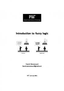
This section is devoted to some items of the L. A. Zadeh’s fuzzy logic agenda mentioned in Section 1.3. Our aim is to prepare some notions used later and to give the reader a clearer understanding to what we are speaking about. The section may be omitted in first reading. Linguistic variable. One of the fundamental concepts introduced by L. A. Zadeh in [ 141] is that of linguistic variable. It is the quintuple hX, T (X), U, G, M i, where X is the name of the variable, T (X) is the set of its values (term set) which are linguistic expressions (syntagms 9 ), U is the universe, G syntactical rule using which we can form syntagms A, B, . . . ∈ T(X), and M is semantical rule, using which every syntagm A ∈ T (X) is assigned its meaning being a fuzzy set A in the universe U , A ⊂ U . ∼ A typical example of the linguistic variable is X := Age. Its term set T (Age) consists of the syntagms such as young, very young, medium age, quite old, more or less young, not old but not young, etc. The universe U ⊆ R is some set of real numbers (note that we may speak about age of various things). The syntactic rule G may be a context-free grammar. The semantic rule M assigns meaning to the terms from T (Age) being various modifications of fuzzy sets depicted on Fig. 1.2. Clearly, there is a lot of other linguistic variables, such as “height, size, temperature, press”, etc.

9A

syntagm is any part of the sentence having a special meaning and formed according to the grammatical rules.


13

1 “young”

“medium age”

50

“old”

90(years)

Figure 1.2. Possible forms of the fuzzy sets assigned as the meaning to the basic syntagms “small”, “medium age”, “old” from T (Age).

Approximate reasoning. Linguistic variables have a quite wide scope of applications. The most important is their use in the approximate reasoning scheme, such as the behaviour of the car driver below: Condition:

Observation: Conclusion:

IF the obstacle is near AND the car speed is big THEN break very much IF the obstacle is far AND the car speed is rather small THEN break a little the obstacle is quite near AND the car speed is big break quite much

This scheme contains vague expressions both in the condition consisting of the so called fuzzy IF-THEN rules, as well as in the observation. Note that such scheme is quite natural for the human mind. As a matter of fact, when driving a car the outer conditions vary so much that we could hardly be able to drive without ability to cope with vaguely stated rules. This is a very strong feature of our mind possible mainly due to its ability to cope with the vagueness phenomenon. Any attempt to give precise solution of tasks like this (think, e.g. about solution of the parking a car) necessarily fails. And it is a great challenge to find a formal system enabling to mimic human mind (at least in approximate reasoning schemes like that above). Fuzzy logic offers a model of the above approximate reasoning scheme. The original proposal of L. A. Zadeh is the so called generalized modus ponens. In Chapter 5, we present the concept of fuzzy logic in broader sense (FLb) which includes the approximate reasoning scheme, but its goal is more general — to model natural human reasoning, in which principal role is played by natural language. Fuzzy quantifiers. Even more complicated situation is faced when using fuzzy quantifiers, i.e. words or syntagms such as “many, most, often, almost, quite much”, etc. For example, we might extend the above scheme by the following rule: In danger, most obstacles should be overcome left, provided that no car is approaching.

Other example with fuzzy quantifiers can be: Many young people like modern music but few of them play an instrument. How many of all young people like modern music and play an instrument?

14


the concept of linguistic variable presented above is not fully satisfactory. The meaning of syntagms depends also on the context, yet there are some general laws inside. One of the reasons for the criticism is neglecting of the concepts of intension and extension. Intension of the meaning, roughly speaking, is the property contained in it. It does not depend on the context and expresses the very content of the meaning. Extension is the reflection of the intension in the universe and it leads to groupings of objects. Thus, for example, the intension of “young” presents itself in various worlds equally but leading to various groupings of “young objects”. Apparently, “young dog” has the meaning different from “young man” and even the latter may be different in Africa, Europe, or Japan. One immediately sees that most of the examples given above have been demonstrated on extensions, but with intensions on mind. The concept of the linguistic variable apparently deals only with extensions. To make it to fit better the linguistic theory, it is necessary to encompass also the concept of intension. The necessity to include linguistic semantics in the fuzzy logic led to the concept of the fuzzy logic in broader sense (FLb) where the intension is interpreted as a special fuzzy set of formulas. The extension is then its interpretation in various models (cf. Chapter 6). On the basis of it, a model of the linguistic semantics of a selected part of natural language consisting of the so called evaluating syntagms is elaborated. Let us stress that FLb is based on FLn, which provides necessary tools for making the inference schemes to work, and for proving some reasonable properties of them. FLb has, in our opinion, a potential for the development of the Zadeh’s fuzzy logic agenda and for proving interesting properties of it.

2

ALGEBRAIC STRUCTURES FOR LOGICAL CALCULI

As stated in the previous chapter, fuzzy logic presented in this book is mostly truth functional. The truth values are taken from the support of some algebraic structure and its operations are assigned to the logical connectives. Hence, the truth value of a compound formula is obtained using algebraic operations of the given algebra from its constituents. In this chapter, we present an overview of basic algebraic structures, which are used for truth values of various logical calculi. The first two sections contain presentation of Boolean algebras, residuated lattices and MV-algebras. All these structures play an important role in the development of logic. The third section is an overview of specific operations in the interval [0, 1] called t-norms, which are natural interpretation of the connective AND in fuzzy logic. The chapter is closed with overview of topos theory and lattice of subobjects in topos. Notational convention. The following notational convention will be employed throughout this book. If there is some correspondence among various kinds of mathematical objects then they will be denoted by the same letter from different font families. For example, if L is an algebra then its support is denoted by the corresponding roman letter L. In general, A, A, A, a denote objects being somehow related to each other. The symbol := means “is defined by”. By N we denote the set of natural numbers. The sets of rational and real numbers are denoted by Q and R, respectively. The expression “if and only if” is usually written as “iff”. Similarly, the 15

16


expression “with respect to” is often shortened as “w.r.t”. The symbols I, J, K usually serve as auxiliary to denote some (arbitrary) sets of indices (subscripts, superscripts, etc.). Besides this we assume that the reader is acquainted with the common mathematical notation. However, if we consider a symbol to be more specific then we introduce in the text. 2.1 2.1.1

Algebras for Logics Boolean algebras

We start this section with the study of abstract Boolean algebras. Their definition will be given using the full list of generating identities. We choose this approach among others, especially to be able to show the existing close relation between the generating identities and logical axioms of classical logical calculus. Moreover, the way for generalization leading to non-classical logical algebras such as MV-algebras, etc. is thus opened. Having on mind the second purpose, we will suggest two different definitions of a Boolean algebra. The first, most familiar one, uses lattice operations, and the second one uses ring operations. It is worth to be mentioned that in the case of a Boolean algebra, both approaches are interchangeable while in other, non-classical logical algebras, both of them are present. We will conclude the subsection with a variant of the representation theorem given by Tarski and show some consequences of it leading to normal forms. Boolean algebra as a special lattice. A Boolean algebra is introduced here as a lattice with special properties. This is the way well established in the literature (see e.g. [ 16]). For better readability, we recall that a lattice is an ordered set containing with each pair of elements their least upper bound (supremum) as well as the greatest lower bound (infimum). Since sup and inf are uniquely determined, they can be considered as two binary operations, namely ∨ (join) and ∧ (meet) respectively, so that the lattice becomes at the same time an algebra endowed with these two operations. In symbols, we write sup(a, b) = a ∨ b,

inf(a, b) = a ∧ b.

The following lemma exposes the basic lattice properties. These are normally included in its definition though they can easily be deduced from the definition given above. Lemma 2.1 Let L be a lattice. Then the following identities (also called laws) are true: a ∨ (b ∨ c) = (a ∨ b) ∨ c, a ∨ b = b ∨ a,

a ∧ (b ∧ c) = (a ∧ b) ∧ c, (associativity) a ∧ b = b ∧ a,

a ∨ (a ∧ b) = a,

a ∧ (a ∨ b) = a,

a ∨ a = a,

a ∧ a = a.

(2.1)

(commutativity) (2.2) (absorption)

(2.3)

(idempotency)

(2.4)


17

Conversely, if L = hL, ∨, ∧i is an algebra with two binary operations fulfilling (2.1)– (2.3) then an ordering ≤ could be defined on L as follows: a ≤ b iff

a ∨ b = b,

(equivalently a ∧ b = a),

so that the ordered set (L, ≤) forms a lattice where sup(a, b) = a ∨ b and

inf(a, b) = a ∧ b.

The proof of this lemma is not complicated and uses only the definition and the uniqueness of sup and inf. Important instances of lattices are distributive lattices and lattices with complements. Definition 2.1 A lattice L is distributive if the following identities (distributivity laws) are true: a ∨ (b ∧ c) = (a ∨ b) ∧ (a ∨ c),

(2.5)

a ∧ (b ∨ c) = (a ∧ b) ∨ (a ∧ c).

(2.6)

Definition 2.2 A lattice L is a lattice with complements if it has the least element 0 and a unary operation of complement ‘0 ’, so that the following identities are true: a00 = a, 0

0

0

(a ∨ b) = a ∧ b , 0

a ∧ a = 0.

(law of double negation)

(2.7)

(the first de Morgan law)

(2.8)

(law of contradiction)

(2.9)

Let us put 1 = 00 . It is easy to show that 1 is the greatest element of L. The interested reader can find more information about lattices, for example, in [ 9, 37]. Definition 2.3 A Boolean algebra is a distributive lattice with complements. With respect to this definition, a Boolean algebra is also called a Boolean lattice. The full list of the generating identities is given by (2.1)–(2.9). In symbols, a Boolean algebra is denoted by L = hL, ∨, ∧,0 , 0, 1i. In the theory of Boolean algebras, the complement is usually denoted by ‘0 ’. However, one may also meet the symbol ‘¯’ and in the papers on logic, the symbol ‘¬’. The latter one is most often used in this book. A Boolean algebra L is finite if its support L is finite. In the sequel, we will refer to the following examples of Boolean algebras. Example 2.1 (Boolean algebra for classical logic) This algebra serves for the truth evaluation of formulas of classical logic. Two values, namely “false” and “true”, which are usually denoted by 0 and 1,

18


respectively, are sufficient for this purpose. Thus, the Boolean algebra in this case is based on the set consisting of two elements only, i.e. LB = h{0, 1}, ∨, ∧, ¬i where the operations “∨, ∧, ¬” are defined using the following tables: ∨

0

1

∧

0

1

¬

0 1

0 1

1 1

0 1

0 0

0 1

0 1

1 0

Since these operations are heavily used in classical logic, they are known under the names corresponding to the respective logical connectives “disjunction”, “conjunction” and “negation”. The other two known logical connectives of “implication” and “equivalence” enrich the set of the basic operations above by → and ↔, respectively defined by the following tables: →

0

1

↔

0

1

0 1

1 0

1 1

0 1

1 0

0 1

Note that the operations →, ↔ can be derived from the basic ones using the following expressions: a → b = a0 ∨ b

a ↔ b = (a → b) ∧ (b → a). 2

Example 2.2 (Boolean algebra of subsets) Let A be an arbitrary nonempty set and P (A) = {0, 1}A be a set of all its subsets. The Boolean algebra based on this set is B(A) = h{0, 1}A , ∪, ∩,¯, ∅, Ai where “∪”,“∩” and “¯” are the ordinary operations of union, intersection and complement, respectively. 2 Example 2.3 ((Algebra of Boolean functions)) Let P2n , n ≥ 1, be a set of all functions f (x1 , . . . , xn ) defined on {0, 1} and taking values from this set. Such functions are called Boolean. The respective Boolean algebra based on P2n is LnP = hP2n , ∨, ∧, ¬, 0, 1i where the operations “∨”, “∧” and “¬” are defined pointwise, and 0, 1 denote the respective constant functions. 2 Example 2.4 (Boolean algebra of propositions) This algebra is based on the set of all propositions, that is, the sentences which can be evaluated either by “true” or by “false”. Every two propositions P , Q


19

are assigned the following three compound ones, namely “P or Q”, “P and Q”, “not P ” being the result of the basic operations “∨”, “∧” and “¬”, respectively. Two propositions are equal if their evaluations coincide. The least element 0 of this algebra is a proposition evaluated by “false”. 2 Among all Boolean algebras, special attention will be paid to those having generating identities true for any (infinite) families of their elements. Definition 2.4 A Boolean algebra L is complete if the underlying lattice is complete that is, each subset has the least upper bound as well as the greatest lower bound. In this case 0 = inf L = sup ∅ and 1 = sup L = inf ∅. Definition 2.5 A Boolean algebra is completely distributive if for any family of its elements (aij )i∈I,j∈J the equality   ! ^ _ _ ^  aij  = aiα(i) i∈I

j∈J

α∈J I

i∈I

holds, provided that the elements defined on both its sides exist. The example of complete and completely distributive Boolean algebra is given by B(A) (see Example 2.2) for any set A. Boolean algebra as a special ring. In comparison with the previous way of introducing of the Boolean algebra, the algebra we suggest now is not so popular. However, it is important for us due to necessity for further generalizations. Definition 2.6 A Boolean ring is a commutative ring R = hL, +, ·,0 , 0, 1i with the unary operation of complement a0 = 1 − a, unit element, and such that every element is idempotent, i.e., a · a = a. The set of generating identities for a Boolean ring is the following: a + (b + c) = (a + b) + c,

a · (b · c) = (a · b) · c,

a + b = b + a,

a · b = b · a,

a + (−a) = 0,

a · a = a,

a + 0 = a,

a · 1 = a,

(2.10)

a · (b + c) = a · b + a · c. Lemma 2.2 In a Boolean ring, each element is equal to its opposite, i.e. a = −a. Proof: Using (2.10), we obtain a sequence of equalities, true for any two elements a, b, namely a+b = (a+b)·(a+b) = a·a+a·b+b·a+b·b = a+a·b+b·a+b.

20


This gives a · b + b · a = 0. Setting a = b, the equations a + a = 0 and a = −a follow. 2 The following proposition establishes the equivalence between Boolean algebra and ring. Lemma 2.3 Let R = hL, +, ·,0 , 0, 1i be a Boolean ring and let a ∨ b = a + b + a · b, a ∧ b = a · b. Then the algebra L = hL, ∨, ∧,0 , 0, 1i is Boolean. Conversely, if in a Boolean algebra L = hL, ∨, ∧,0 , 0, 1i the ring operations are defined using the formulas a + b = (a ∧ b0 ) ∨ (a0 ∧ b), a·b=a∧b then the algebra R = hL, +, ·,0 , 0, 1i is a Boolean ring. Proof: To prove both parts of this lemma, it is sufficient to derive the first group of generating identities from the second one and vice-versa. As an example, we will demonstrate it by choosing one identity from each side. (a) The distributivity of ∨ with respect to ∧. For the proof, we will transform each side of the identity to the same expression. a ∨ (b ∧ c) = a + b · c + a · b · c, (a ∨ b) ∧ (a ∨ c) = (a + b + a · b) · (a + c + a · c) = = a · a + a · c + a · a · c + b · a + b · c + b · a · c+ +a·b·a+a·b·c+a·b·a·c= = a + b · c + a · b · c. (b) The distributivity of · with respect to +. The method of the proof will be the same as above. a · (b + c) = a ∧ ((b ∧ c0 ) ∨ (b0 ∧ c)), (a · b) + (a · c) = ((a ∧ b) ∧ (a ∧ c)0 ) ∨ ((a ∧ b)0 ∧ (a ∧ c)) = = (a ∧ b ∧ a0 ) ∨ (a ∧ b ∧ c0 ) ∨ (a0 ∧ a ∧ c) ∨ (b0 ∧ a ∧ c) = = a ∧ ((b ∧ c0 ) ∨ (b0 ∧ c)). 2 Lemma 2.4 In a Boolean ring with lattice operations ∨ and ∧, the following identities are true: (a) a + a0 = 1,


21

(b) a ∧ b = (a + b0 ) · b, (c) a ∨ b = a · b0 + b, (d) (a + b0 ) · b = (b + a0 ) · a, (e) a · b0 + b = b · a0 + a. Proof: (a) a + a0 = a + (1 − a) = 1 + (a − a) = 1, (b) (a + b0 ) · b = (a + (1 − b)) · b = a · b + b − b · b = a · b + (b − b) = a · b = a ∧ b, (c) a · b0 + b = a · (1 − b) + b = a − a · b + b = a + b + a · b = a ∨ b, (d) follows from (b), (e) follows from (c). 2 Duality. Note that the generating identities (2.1)–(2.9) of a Boolean algebra are such that if we at the same time replace 0 by 1, 1 by 0, ∨ by ∧ and ∧ by ∨, then we again obtain generating identities. This rule is known as the duality principle. Equalities obtained one from the other by applying the duality principle are called dual . Validity of this principle can easily be checked for (2.1)– (2.6) since both, formula as well as its dual are there present. We show that (2.8) and (2.9) have also their duals and that they are identities. Indeed, from the identity (a ∨ b)0 = a0 ∧ b0 (the first de Morgan law) we can easily deduce the identity a0 ∨ b0 = (a0 ∨ b0 )00 = (a00 ∧ b00 )0 = (a ∧ b)0 , which is called the second de Morgan law. Similarly, from the identity a ∧ a0 = 0 (the law of contradiction) we deduce the dual identity 1 = (a ∧ a0 )0 = (a00 ∧ a0 )0 = (a0 ∨ a)00 = a0 ∨ a, which is called the law of the excluded middle. Important application of the duality principle gives us the representation of each element of a Boolean algebra in two normal forms. We are going to show it below. Representation theorem and normal forms. Among the examples of a Boolean algebra, the most important is Example 2.2 because it serves as a canonical representation of any Boolean algebra. The following theorem known as the representation theorem justifies this assertion. Usually, this theorem is connected with the name of M. H. Stone as he suggested the most general formulation. Here we present a simpler version first proved by A. Tarski. Theorem 2.1 Every complete and completely distributive Boolean algebra is isomorphic to B(A) for some set A. Proof: Let L be the given algebra with the set of elements L. The following evident equality ^ 1= (a ∨ a0 ) a∈L

22


could be rewritten using the complete distributivity into   !  _ ^ ^  1= a ∧ b0  . C∈2L

(2.11)

b6∈C

a∈C

V V Put t(C) = ( a∈C a) ∧ ( b6∈C b0 ). We show that t(C) is either 0 or an atom of the algebra L (i.e. minimal element different from 0). Indeed, suppose that t(C) 6= 0 but there exists c ∈ L, c 6= 0 and c ≤ t(C). In general, two cases are possible: (a) c ∈ C, whence t(C) ≤ c and consequently, c = t(C); (b) c 6∈ C, whence t(C) ≤ c0 which together with c ≤ t(C) gives c ≤ c0 . Consequently, c = c ∧ c0 = 0, which contradicts with the choice of c. Let A denote the set of all atoms t(C) 6= 0. We show that L is isomorphic to B(A). To do it, we assign to every subset of the set A its least upper bound in L (which exists due to the completeness of L) and conversely, to each W element c ∈ L we assign the subset {t(C) | t(C) ≤ c}. By (2.11), c = c ∧ ( C∈2L t(C)) W and, consequently, c = {t(C) | t(C) ≤ c} or c is the least upper bound of the subset corresponding to it. Hence, we have obtained a one-to-one correspondence between {0, 1}A and L, which, as may easily be seen, preserves the ordering and thus, it is the isomorphism. 2 Corollary 2.1 Every finite Boolean algebra is isomorphic to B(A) for some finite set A. Proof: The proof easily follows from the fact that each finite Boolean algebra is complete and completely distributive. In this case, A is evidently the set of all atoms of the given Boolean algebra. 2 Remark 2.1 A generalization of Corollary 2.1 stating that every Boolean algebra is isomorphic to some algebra of sets is known as Stone representation theorem. Corollary 2.2 Let L be a finite Boolean algebra and A be its set of atoms. Then each element x of L can uniquely be represented in two forms, namely _ ^ x= (a ∧ b0 ), (2.12) a∈A a≤x

x=

^ a∈A a≤x0

b∈A\{a}

(a0 ∨

_

b)

(2.13)

b∈A\{a}

which are called the perfect disjunctive normal form and the perfect conjunctive normal form, respectively. Proof: First, we W prove (2.12). Let x be an arbitrary element from L. Then the equality x = a∈A a directly follows from the proof of Theorem 2.1. Hence, a≤x


23

it is sufficient to prove that if a, b ∈ A and b ∈ A \ {a} then a ∧ b0 = a. Indeed, since a and b are atoms and b ∈ A \ {a} then a ∧ b = 0 which finally gives a = a ∧ (b ∨ b0 ) = (a ∧ b) ∨ (a ∧ b0 ) = 0 ∨ (a ∧ b0 ) = (a ∧ b0 ). To prove (2.13), it is sufficient to represent the complement x0 in the perfect disjunctive normal form and then apply the first de Morgan law (2.8): x0 =

_

^

(a ∧

a∈A a≤x0

b0 ),

b∈A\{a}

0

 _ x00 =  (a ∧ a∈A a≤x0

^

x=

a∈A a≤x0

a0 ∨

and finally

b∈A\{a}

 ^

 b0 ) , 

_

b .

b∈A\{a}

2 2.1.2

Residuated lattices and MV-algebras

In order to have more than two values for evaluation of formulas, many attempts have been done to generalize the classical algebra for logic (see Example 2.1). On this way, two special structures took a distinguished role, namely residuated lattices and MV-algebras. In this subsection, we will briefly overview the main properties of them. Suppose that the set L of truth values forms a lattice with respect to inf (∧) and sup (∨) and it contains the least (0) and the greatest (1) elements. It has been demonstrated (see, e.g. [ 57]) that there is no possibility to define a unary operation of complement on L so that all the laws (2.1)–(2.9) of the Boolean algebra hold true. Therefore, on the way of generalization we may only increase the number of operations and distribute various laws among them. We will see that in the case of MV-algebras, this requires to add two specific operations of multiplication (⊗) and addition (⊕) and then to share the full list of Boolean laws over five operations ∨, ∧, ⊕, ⊗, ¬ and two constants 0, 1. Moreover, the operations ⊕ and ⊗ have at the same time some of the properties of the ring operations taken from the Boolean rings. As may be expected, if L degenerates to two-element set then the operations ⊕ and ⊗ coincide with ∨ and ∧, respectively. A residuated lattice can be placed between Boolean and MV- algebras. The list of its operations contains, besides the lattice ones, also two additional operations called multiplication and residuation. In the case that L = {0, 1}, these coincide with ∧ and →, respectively. The results in this subsection are due to many authors. Among them, let us name L. P. Belluce, A. DiNola, P. Hájek, U. Höhle, S. Gottwald, D. Mundici, J. Pavelka, and others. A lot of results, especially those concerning residuated lattices, are taken from the book [ 51].

24


Residuated lattices. Definition 2.7 A residuated lattice is an algebra L = hL, ∨, ∧, ⊗, →, 0, 1i.

(2.14)

with four binary operations and two constants such that (i) hL, ∨, ∧, 0, 1i is a lattice with the ordering ≤ defined using the operations ∨, ∧ as usual, and 0, 1 are its least and the greatest elements, respectively; (ii) hL, ⊗, 1i is a commutative monoid, that is, ⊗ is a commutative and associative operation with the identity a ⊗ 1 = a; (iii) the operation ⊗ is isotone in both arguments; (iv) the operation → is a residuation operation with respect to ⊗, i.e. a ⊗ b ≤ c iff

a ≤ b → c.

(2.15)

We see that in comparison with the ordinary lattice, this structure is enriched by a special couple h⊗, →i of operations called the adjoint couple. The defining relation (2.15) is called the adjunction property. We will call ⊗ the multiplication and → the residuation. Let us remark that there are several other names for residuated lattice, namely integral commutative, residuated l-monoid (or cl-monoid, if it is complete); residuated commutative Abelian semigroup; complete lattice ordered semigroup. The term “residuated lattice” has been introduced by Dilworth and Ward in [ 18, 19]. The following examples of residuated lattices will be quite often referred to. Example 2.5 (Boolean algebra for classical logic, cf. Example 2.1) LB = h{0, 1}, ∨, ∧, →, 0, 1i where → is the classical implication, is the simplest residuated lattice (the multiplication ⊗ = ∧). In general, every Boolean algebra is a residuated lattice when putting a → b = a0 ∨ b. 2 ¨ del algebra) Example 2.6 (Go LG = h[0, 1], ∨, ∧, →G , 0, 1i where the multiplication ⊗ = ∧ and ( a →G b =

1 b

if a ≤ b, if b < a.

(2.16)

G¨ odel algebra is a special case of the Heyting algebra used in intuitionistic logic. We will return to Heyting algebras in Subsection 2.4.3. 2


25

Example 2.7 (Goguen algebra) LP = h[0, 1], ∨, ∧, , →P , 0, 1i where the multiplication = · is the ordinary product of reals and ( 1 if a ≤ b, a →P b = b if b < a. a

(2.17) 2

Example 2.8 (Lukasiewicz algebra) LL = h[0, 1], ∨, ∧, ⊗, →L , 0, 1i

(2.18)

where a ⊗ b = 0 ∨ (a + b − 1), a →L b = 1 ∧ (1 − a + b).

(Lukasiewicz conjunction)

(2.19)

(Lukasiewicz implication)

(2.20) 2

Example 2.9 (Residuated lattice of [0, 1]-valued functions) Let X be a nonempty set. For each two functions f, g ∈ [0, 1]X we put (f ∨ g)(x) = f (x) ∨ g(x), (f ∧ g)(x) = f (x) ∧ g(x),

(f ⊗ g)(x) = f (x) ⊗ g(x), (f → g)(x) = f (x) → g(x)

(2.21) (2.22)

for all x ∈ X where ∨, ∧, ⊗, → are the corresponding operations of the Lukasiewicz algebra (Example 2.8). Furthermore, let 1 and 0 be constant functions taking the values 1 and 0, respectively. Then Lf unc (X) = h[0, 1]X , ∨ , ∧ , ⊗ , → , 0, 1i 2

is a residuated lattice.

The subsequent lemma shows some commonly used properties of residuated lattices. Lemma 2.5 Let L be a residuated lattice given by (2.14). Then for every a, b, c ∈ L the following holds true. (a) a ⊗ b ≤ a,

a ⊗ b ≤ b,

a ⊗ b ≤ a ∧ b,

(b) b ≤ a → b, (c) a ⊗ (a → b) ≤ b,

b ≤ a → (a ⊗ b),

(d) if a ≤ b then c→a≤c→b

(isotonicity in the second argument),

a→c≥b→c

(antitonicity in the first argument),

26


(e) a ⊗ (a → 0) = 0, (f) a → (b → c) = (a ⊗ b) → c, (g) a ≤ b iff

a → b = 1,

a = 1 → a,

(h) (a ∨ b) ⊗ c = (a ⊗ c) ∨ (b ⊗ c), (i) a ∨ b ≤ ((a → b) → b) ∧ ((b → a) → a). Proof: (a) is an easy consequence of isotonicity, and (b)–(c) of the adjunction property. (d) Using (c), we obtain c⊗(c → a) ≤ a ≤ b, which follows the first inequality. The second inequality immediately follows from a ⊗ (b → c) ≤ b ⊗ (b → c) ≤ c. (e)–(f) follow from the adjunction and (c). (g) a ⊗ 1 ≤ b, i.e. 1 ≤ a → b. The second part is obtained from 1 → a = 1 ⊗ (1 → a) ≤ a ≤ 1 → a due to (b). (h) a⊗c ≤ (a∨b)⊗c and b⊗c ≤ (a∨b)⊗c. Thus, (a⊗c)∨(b⊗c) ≤ (a∨b)⊗c. On the other hand, a ⊗ c ≤ (a ⊗ c) ∨ (b ⊗ c) and b ⊗ c ≤ (a ⊗ c) ∨ (b ⊗ c). Then (a ∨ b) ≤ c → (a ⊗ c) ∨ (b ⊗ c) by the adjunction and properties of supremum. Again by the adjunction, we obtain (a ∨ b) ⊗ c ≤ (a ⊗ c) ∨ (b ⊗ c). (i) Using (a), (c) and (h), we obtain the inequality (a ∨ b) ⊗ (a → b) = (a⊗(a → b))∨(b⊗(a → b)) ≤ b and similarly for a. Hence, a∨b ≤ (a → b) → b as well as a ∨ b ≤ (b → a) → a which gives the required inequality. 2 To be convinced that a residuated lattice is a generalization of the Boolean one, let us prove the following lemma. Lemma 2.6 Let L be a residuated lattice given by (2.14). If 1 = a ∨ (a → 0) holds for every a ∈ L then L is a Boolean lattice and ⊗ = ∧. Proof: It is necessary to prove that the distributive law as well as the laws of double negation, de Morgan and contradiction are valid. We will prove idempotency and the first two mentioned properties. Put a0 = a → 0. Then using Lemma 2.5(e) and (h) we obtain a = a ⊗ 1 = a ⊗ (a ∨ a0 ) = (a ⊗ a) ∨ 0 = a ⊗ a and thus, ⊗ is idempotent. Then a ∧ b = (a ∧ b) ⊗ (a ∧ b) ≤ a ⊗ b, i.e. ⊗ = ∧. From this and Lemma 2.5(h), the distributivity easily follows. The law of double negation is proved by the following sequence of equalities: a = a ∧ 1 = a ∧ (a0 ∨ a00 ) = (a ∧ a0 ) ∨ (a ∧ a00 ) = a ∧ a00 = = (a ∧ a00 ) ∨ (a0 ∧ a00 ) = a00 ∧ (a ∨ a0 ) = a00 ∧ 1 = a00 . 2


27

Additional operations and their properties. To be used as an algebra for many-valued logic, residuated lattices should be completed by additional operations corresponding (among others) to the logical connectives. Analogously as in classical logic, they can be obtained as derived operations from the basic ones. ¬a = a → 0

(negation),

(2.23)

(biresiduation),

(2.24)

(addition),

(2.25)

a = a ⊗ ··· ⊗ a | {z }

(n-fold multiplication),

(2.26)

na = a ⊕ · · · ⊕ a | {z }

(n-fold addition).

(2.27)

a ↔ b = (a → b) ∧ (b → a) a ⊕ b = ¬(¬a ⊗ ¬b) n

n−times

n−times

It follows from the antitonicity of → in the first variable (Lemma 2.5(d)) that the negation is order reversing, i.e. if a ≤ b then ¬b ≤ ¬a.

(2.28)

Lemma 2.7 Let L be a residuated lattice given by (2.14). Then the following holds true for every a, b, c, d ∈ L. (a) a ↔ 1 = a,

a = b iff

a ↔ b = 1,

(b) (a ↔ b) ∧ (c ↔ d) ≤ (a ∧ c) ↔ (b ∧ d), (c) (a ↔ b) ∧ (c ↔ d) ≤ (a ∨ c) ↔ (b ∨ d), (d) (a ↔ b) ⊗ (c ↔ d) ≤ (a ⊗ c) ↔ (b ⊗ d), (e) (a ↔ b) ⊗ (c ↔ d) ≤ (a → c) ↔ (b → d), (f) (a ↔ b) ⊗ (b ↔ c) ≤ (a ↔ c). Proof: We will prove only one of the inequalities. The other ones are proved using analogous technique and thus, left to the reader. (b) For any a, b, c, d ∈ L we have ((a ↔ b) ∧ (c ↔ d)) ⊗ (a ∧ c) ≤ ((a → b) ∧ (c → d)) ⊗ (a ∧ c) ≤ ((a → b) ⊗ a) ∧ ((c → d) ⊗ c) ≤ b ∧ d. Hence, (a ↔ b) ∧ (c ↔ d) ≤ (a ∧ c) → (b ∧ d). By symmetry of biresiduation, we obtain also (a ↔ b) ∧ (c ↔ d) ≤ (b ∧ d) → (a ∧ c) which yields the required inequality. 2 The following operation is trivial in Boolean lattices and thus, it makes sense only for the residuated ones. It partially compensates the absence of the law of idempotency and is called the square root. This concept has been introduced by U. H¨ ohle.

28


Definition 2.8 Let L be a residuated lattice with the support L. If there exists a unary √ operation : L −→ L fulfilling the following properties √ √ (S1) a ⊗ a = a, √ (S2) b ⊗ b ≤ a implies b ≤ a for every a, b ∈ L, then we say that L has square roots. √ Obviously, is uniquely determined. Example 2.10 Lukasiewicz algebra LL has square roots given by √

a=

a+1 2

where a ∈ [0, 1]. In general, √

√ √ a + 2k − 1 k ··· a = 2 a = . | {z } 2k k−times

Therefore,

√

√ 2k − 1 1 2k and ¬ 0 = k . k 2 2 Goguen algebra LP has square roots coinciding with the ordinary square roots of real numbers. 2 2k

0=

The following lemma summarizes some of the properties of square roots. Lemma 2.8 Let L be a residuated lattice with square roots. The following holds for every a, b ∈ L. √ √ √ (a) a ≤ a, a ≤ b implies a ≤ b, √ √ √ (b) a ⊗ b ≤ a ⊗ b, √ √ √ (c) a → b = a → b, √ √ √ (d) a ∧ b = a ∧ b, √ √ (e) a ∧ b ≤ a ⊗ b ≤ a ∨ b. Linear ordering and completeness of residuated lattices. Lattice completeness is a property usually required when evaluating quantified formulas. As we will see, the completeness provides also a natural possibility how the residuation operation can be directly defined using the multiplication, or viceversa (see Lemma 2.9(a),(b)). Definition 2.9 Let L be a residuated lattice.


29

(i) L is linearly ordered if a ≤ b or b ≤ a holds for every a, b ∈ L. (ii) L is complete if the underlying lattice is complete. (iii) L is divisible if a ≤ b implies existence of c ∈ L such that b ⊗ c = a. Lemma 2.9 Let L be a complete residuated lattice. Then the following identities hold for every a, b ∈ L and sets {ai | i ∈ I}, {bi | i ∈ I} of elements from L over arbitrary set of indices I. W (a) a → b = {x | a ⊗ x ≤ b}, V (b) a ⊗ b = {x | a ≤ b → x}. W W (c) ( i∈I ai ) ⊗ b = i∈I (ai ⊗ b), V V (d) i∈I (a → bi ) = a → ( i∈I bi ), V W (e) i∈I (ai → b) = ( i∈I ai ) → b, W W (f) i∈I (a → bi ) ≤ a → ( i∈I bi ), W V (g) i∈I (ai → b) ≤ ( i∈I ai ) → b. Proof: Put K = {x | a ⊗ x ≤ b}. W (a) By adjunction, x ≤ a → b for every x ∈ K. Hence, x∈K x ≤ a → b. Vice-versa, W a ⊗ (a → b) ≤ b (by Lemma 2.5 (c)), i.e. a → b ∈ K, which gives a → b ≤ x∈K x. (b)–(e) are proved analogously. (f) and (g) are the consequences of the isotonicity of → in the second argument and antitonicity in the first one. 2 If the index set I is finite then the properties (c)–(g) of this lemma hold in every residuated lattice. A special case of residuated lattices are BL-algebras1 , which have been introduced by P. H´ ajek to develop a kernel logical calculus, which would be included in various kinds of many- valued logical calculi. From the algebraic point of view, BL-algebras enrich residuated lattices by two special properties given in the definition below. Definition 2.10 Let L be a residuated lattice. It is called the BL-algebra if the following holds for every a, b ∈ L. (i) a ⊗ (a → b) = a ∧ b, (ii) (a → b) ∨ (b → a) = 1 (prelinearity axiom). Lemma 2.10 (a) A linearly ordered residuated lattice L is a BL-algebra iff it fulfils condition (i) of Definition 2.10. 1 ‘BL’

means “basic logic”.

30


(b) If a linearly ordered residuated lattice L is divisible then it is a BL-algebra. (c) The following identity holds true in any BL-algebra a ∨ b = ((a → b) → b) ∧ ((b → a) → a). Proof: (a) We must check the prelinearity axiom. If L is linearly ordered then either a ≤ b or b ≤ a holds for every a, b ∈ L. By Lemma 2.5(g) we obtain the assertion. (b) By (a) it is sufficient to prove the prelinearity. Suppose a ≤ b, then a ∧ b = a = a ⊗ 1 = a ⊗ (a → b). Now, let b < a. Then a ∧ b = b and a ⊗ (a → b) ≤ b. Since L is divisible, there is c such that a ⊗ c = b. The assertion then follows from the adjunction and the isotonicity of ⊗. (c) The corresponding inequality is obtained by Lemma 2.5(i). We have to prove the opposite one. Indeed, using the prelinearity we have (((a → b) → b) ∧ ((b → a) → a)) ⊗ ((a → b) ∨ (b → a)) = = ((a → b) ⊗ (((a → b) → b) ∧ ((b → a) → a)))∨ ∨((b → a) ⊗ (((b → a) → a) ∧ ((a → b) → b))) ≤ ≤ ((a → b) ⊗ ((a → b) → b)) ∨ ((b → a) ⊗ ((b → a) → a)) ≤ b ∨ a. 2 Remark 2.2 It is not difficult to deduce from the proof of (b) that the divisibility property is equivalent in residuated lattices with the condition (i) of Definition 2.10. Example 2.11 The Lukasiewicz, G¨ odel and Goguen algebras from Example 2.5 are BL-algebras. Indeed, by Lemma 2.10(a) it is sufficient to prove the identity a⊗(a → b) = a∧b. Let a ≤ b. Then a ∧ b = a and in all three cases a → b = 1 and thus, a ⊗ (a → b) = a. Let b < a. Then a ∧ b = b and we obtain for the respective algebras the following. LP : a ⊗ (a → b) = a · ab = b. LG : a ⊗ (a → b) = a ∧ b = b. LL : a ⊗ (a → b) = a + (1 − a + b) − 1 = b. 2 MV-algebras. The notion of MV-algebra2 was introduced by C. C. Chang [ 12] for an algebraic system, which would correspond to the ℵ0 -valued propositional calculus. MV-algebras have been developed as generalizations of Boolean algebras to be able to transfer the Boolean prime ideal theorem to the general case and thus, to prove completeness of the ℵ0 -valued logic. However, it turned out that MV-algebras as well as BL-algebras stand for the algebraic structures of truth values for various non-classical logical calculi including fuzzy logics. As in each example of the algebras presented above, the MV-algebra can also be

2 ‘MV’

means “many-valued”.


31

treated as a special kind of the lattice supplied with two additional algebraic operations called addition and multiplication. From the algebraic point of view, the MV-algebra differs from the Boolean one by absence of the idempotency law for their algebraic operations (addition and multiplication) and also, by the lack of the law of excluded middle for the lattice operations. It is also worth noticing that there are some common properties of an MValgebra and a Boolean ring. For example, each identity from Lemma 2.4 is valid also in an MV-algebra. From this point of view, an MV-algebra restricted only to algebraic operations can also be treated as a generalization of a Boolean ring. The following definition of an MV-algebra, is not the most economic one. It originates from the definition given by C. C. Chang (see [ 12]). Definition 2.11 An MV-algebra is an algebra L = hL, ⊕, ⊗, ¬, 0, 1i

(2.29)

in which the following identities are valid. a ⊕ b = b ⊕ a,

a ⊗ b = b ⊗ a,

(2.30)

a ⊕ (b ⊕ c) = (a ⊕ b) ⊕ c,

a ⊗ (b ⊗ c) = (a ⊗ b) ⊗ c,

(2.31)

a ⊕ 0 = a,

a ⊗ 1 = a,

(2.32)

a ⊕ 1 = 1,

a ⊗ 0 = 0,

(2.33)

a ⊕ ¬a = 1,

a ⊗ ¬a = 0,

(2.34)

¬(a ⊕ b) = ¬a ⊗ ¬b,

¬(a ⊗ b) = ¬a ⊕ ¬b,

(2.35)

¬0 = 1,

(2.36)

a = ¬¬a, ¬(¬a ⊕ b) ⊕ b = ¬(¬b ⊕ a) ⊕ a.

(2.37)

Most of these identities have obvious interpretation. Note that the identity (2.34) is the law of the excluded middle, the identity (2.35) is the de Morgan law for the operations ⊗ and ⊕ and the first identity of (2.36) is the law of double negation. The last identity (2.37) is specific and it states that the supremum operation is commutative, as can be seen from the definition (2.41) below. The following are the examples of an MV-algebra. Example 2.12 (Lukasiewicz algebra) The Lukasiewicz algebra LL from Example 2.8 is an MV- algebra. It can be written as LL = h[0, 1], ⊕, ⊗, ¬, 0, 1i (2.38) where ⊗ is the Lukasiewicz conjunction defined in (2.19), ⊕ is called the Lukasiewicz disjunction defined by a ⊕ b = 1 ∧ (a + b)

(2.39)

32


2

and ¬ is the negation operation defined by ¬a = 1 − a.

Example 2.13 (MV-algebra of [0, 1]-valued functions) The residuated lattice Lf unc (X) of [0, 1]-valued functions on a nonempty X from Example 2.9 on page 25 is an MV-algebra. 2 Example 2.14 (MV-algebra of dyadic numbers) Let D ⊆ [0, 1] be the set of all rational dyadic numbers on [0, 1], i.e. [ i n | i ∈ {0, 1, . . . , 2 } . D= 2n n∈N

Put a ⊕ b = 1 ∧ (a + b), a ⊗ b = max(0, a + b − 1), ¬a = 1 − a. for all a, b ∈ D. Then D = hD, ⊕, ⊗, ¬, 0, 1i is an MV-algebra, which has the square roots defined in Example 2.10. In particular, it is an MV-subalgebra of the Lukasiewicz algebra LL . 2 Definition 2.12 Let L be an MV-algebra given by (2.29). L is locally finite if to every a 6= 1 there is n ∈ N such that an = 0, or equivalently, to every a 6= 0 there is n ∈ N such that na = 1. (In other terminology this property is called a nilpotentness.) For example, Lukasiewicz MV-algebra LL is locally finite. In the sequel, suppose that we are given some MV-algebra L. Put a≤b

iff ¬a ⊕ b = 1

(2.40)

and verify the properties of partial ordering. Indeed, the reflexivity easily follows from (2.34), the antisymmetry is justified by assuming that ¬a ⊕ b = 1 and ¬b ⊕ a = 1 and deducing that a = ¬¬((¬a ⊕ b) ⊗ a) = ¬(¬(¬a ⊕ ¬¬b) ⊕ ¬a) = ¬(¬(¬b ⊕ ¬¬a) ⊕ ¬b) = = (¬b ⊕ a) ⊗ b = b. The transitivity is left to the reader. The lattice operations can be introduced by a ∨ b = ¬(¬a ⊕ b) ⊕ b = (a ⊗ ¬b) ⊕ b,

(2.41)

a ∧ b = ¬(¬a ∨ ¬b) = (a ⊕ ¬b) ⊗ b.

(2.42)

Moreover, put a → b = ¬a ⊕ b and see that this is a residuation w.r.t. ⊗. Theorem 2.2 (a) Every MV-algebra is a residuated lattice.

33


(b) A residuated lattice L is an MV-algebra iff (a → b) → b = a ∨ b

(2.43)

holds for every a, b ∈ L. (c) A residuated lattice L is an MV-algebra iff it is divisible and keeps the law of double negation (2.36). (d) A BL-algebra is MV-algebra iff it fulfils the law of double negation. Proof: (a) It is necessary to show that the operation → has the properties of residuation. We will demonstrate only adjunction. Using (2.31), (2.35) and (2.36), the inequality a ⊗ b ≤ c is equivalent to a ⊗ b ⊗ ¬c = 0. From the other side, the inequality a ≤ b → c is equivalent to a ⊗ ¬(¬b ⊕ c) = 0. Using (2.35), (2.36) and (2.31) we conclude that the latter is also equivalent to a ⊗ b ⊗ ¬c = 0. (b) If a residuated lattice L fulfils condition (2.43) then by (2.23) we have a = a ∨ 0 = (a → 0) → 0 = ¬¬a, which gives (2.36). The other conditions of MV-algebra can be easily verified. The opposite implication is given by (2.41). (c) see [ 49]. (d) follows from (c) and Remark 2.2 after Lemma 2.10. 2 Corollary 2.3 An MV-algebra is a Boolean algebra if the operation ⊗ (or, equivalently, ⊕) is idempotent. Proof: Since MV-algebra is a residuated lattice then by Lemma 2.6 on page 26, it is sufficient to prove that a ∨ ¬a = 1. Indeed, a ∨ ¬a = (a ⊗ ¬¬a) ⊕ ¬a = (a ⊗ a) ⊕ ¬a = a ⊕ ¬a = 1. 2 Observe that every MV-algebra is a BL-algebra. By Theorem 2.2 (b) both G¨ odel LG as well Goguen LP algebras are not MV-algebras. Indeed, let a < 1 and b = 0. Then in both cases a ∨ b = a but (a → b) → b = 1. The following lemma demonstrates some characteristic, commonly known properties of MV-algebras. In the formulation of them, we use Theorem 2.2(a), according to which the MV-algebra is a residuated lattice. Lemma 2.11 The following are identities in every MV-algebra. (a) (a → b) ∨ (b → a) = 1, (b) (a ∧ b) → c = (a → c) ∨ (b → c), (c) a → (b ∨ c) = (a → b) ∨ (a → c), (d) a → b = ¬b → ¬a. (e) a → (a ⊗ b) = ¬a ∨ b.

34


Proof: We prove (d) and (e). (d) using the definition of → and the law of double negation (2.36), we can write a → b = ¬a ⊕ b = ¬¬b ⊕ ¬a = ¬b → ¬a. (e) Using (2.41) we obtain ¬a ∨ b = (b ⊗ ¬¬a) ⊕ ¬a = a → (a ⊗ b). 2 As usual, an MV-algebra is complete if the underlying lattice is complete. Lemma 2.12 Let L be a complete MV-algebra. Then the following holds true for every a, b ∈ L and sets {ai | i ∈ I}, {bi | i ∈ I} of elements from L over arbitrary set of indices I. W V V W (a) i∈I ai = ¬ i∈I ¬ai , i∈I ai = ¬ i∈I ¬ai , W W V V (b) a ∧ ( i∈I bi ) = i∈I (a ∧ bi ), a ∨ ( i∈I bi ) = i∈I (a ∨ bi ), V V (c) a ⊗ ( i∈I bi ) = i∈I (a ⊗ bi ), W V (d) i∈I (ai → b) = ( i∈I ai ) → b, W W (e) i∈I (a → bi ) = a → ( i∈I bi ). W W Proof: (a) The inequality ai ≤ i∈I ai Wfor all i ∈VI implies ¬ i∈I ai ≤ ¬ai due to (2.28). From it follows that V ¬ i∈I ai ≤ i∈I ¬ai . The opposite inequality is obtained similarly from i∈I ¬ai ≤ ¬ai . The second equality of (a) is left to the reader. W W (b) The inequality i∈I (a ∧ bi ) ≤ a ∧ i∈I bi is obvious. Vice-versa, using Lemma 2.9(c) and (2.42) we have ! ! ! _ _ _ _ _ a∧ bi = a ⊕ ¬ bi ⊗ bi = a⊕¬ bi ⊗ bi ≤ i∈I

i∈I

≤

_

i∈I

((a ⊕ ¬bi ) ⊗ bi ) =

i∈I

i∈I

_

i∈I

(a ∧ bi ).

i∈I

W where the inequality follows from ¬ i∈I bi ≤ ¬bi by (2.28). The second equality of (b) follows from (a). (c) By Lemma 2.9(d) and Lemma 2.11(e) together with just obtained (b), we come to the following ^ ^ ^ ^ a→ (a ⊗ bi ) = (a → (a ⊗ bi )) = (¬a ∨ bi ) = ¬a ∨ bi . i∈I

i∈I

i∈I

i∈I

Let us now multiply both sides by a. By Theorem 2.2(d), L is also a BL-algebra, then the multiplied left- hand side is ! ! ^ ^ ^ a⊗ a→ (a ⊗ bi ) = a ∧ (a ⊗ bi ) = (a ⊗ bi ). i∈I

i∈I

i∈I


35

By Lemma 2.5(h), the multiplied right-hand side is ! ! ^ ^ ^ a ⊗ ¬a ∨ bi = (a ⊗ ¬a) ∨ a ⊗ bi = a ⊗ bi . i∈I

i∈I

i∈I

(d) First, note that ¬(a → b) = a ⊗ ¬b. Then, using (c) we have ! ^ ^ (ai ⊗ ¬b) = ai ⊗ ¬b, i∈I

i∈I

i.e. i∈I ¬(ai → b) = ¬ ( i∈I ai ) → b which gives (d) using the law of double negation (2.36) and (a). (e) is left to the reader. 2 V

2.2

V

Filters and Representation Theorems

In the center of interest of this section there are three representation theorems of MV-algebras: representation by subdirect product of linearly ordered MValgebras, representation by fuzzy sets and representation by the Lukasiewicz algebra. Whenever possible, lemmas and theorems are formulated for the case of general residuated lattice. Since every MV-algebra is also the residuated lattice (cf. Theorem 2.2 on page 32), every property of the latter is obviously valid also for the former. The results presented in this section heavily rely on the results presented by C. C. Chang in [ 12], U. Höhle in [ 48] and R. Cignolli, I. M. L. D’Ottaviano and D. Mundici in [ 84]. Filters and congruences. Filter theory provides one of the fundamental algebraic techniques, which makes it possible to investigate deep and principal characteristics of the underlying algebras. We introduce few basic definitions and also demonstrate a close connection between filters and congruences. Definition 2.13 Let L be a residuated lattice. A subset F ⊆ L is a filter of L if it fulfils the following conditions: (i) 1 ∈ F , (ii) if a ∈ F and a ≤ b then b ∈ F , (iii) if a, b ∈ F then a ⊗ b ∈ F . A filter F is called proper if it does not contain 0. Note that a dual concept of ideal of L can be introduced as well. In our case, it is a matter of preference which one to choose. Thus, we will base our constructions on filters. In the sequel, we suppose that L is a residuated lattice and F is a proper filter of it. Since an MV-algebra is a particular case of a

36


residuated lattice, it inherits all the properties of the latter. In some specific cases, which will be specially indicated, the symbol L will be used to denote an MV- algebra as well. A proper filter F is called prime if a∨b∈F

implies a ∈ F

or b ∈ F.

It can be easily demonstrated that F is prime iff either a → b ∈ F or b → a ∈ F . A proper filter F is called maximal if for any other filter G, F ⊆ G implies F = G. We will call a maximal filter an ultrafilter . The following is the classical lemma concerning the existence of ultrafilters. Lemma 2.13 Every proper filter F can be extended to an ultrafilter containing it. Proof: Let S F = {Fi | i ∈ I} be a chain of filters containing a proper filter F . Obviously, F is a filter containing F . Then use Zorn’s lemma. 2 The lemma below is a good example of the filter based technique. It has also it’s own importance in the proof of the first representation theorem. Lemma 2.14 Let L be an MV-algebra and a ∈ L, a 6= 1. Then there is a prime filter F of L not containing a. Proof: Let a ∈ L and a 6= 1. By F(a) we denote the set of all filters, which do not contain a. Obviously, {1} ∈ F(a) and therefore, F(a) is nonempty. Using Zorn’s lemma, there is a maximal element F in F(a) w.r.t. the ordinary inclusion. We show that F is prime. Suppose the opposite. Let b1 ∨ b2 ∈ F and b1 , b2 6∈ F . Since F is a maximal element in F(a), there are c1 , c2 ∈ F and natural numbers n1 , n2 such that bn1 1 ⊗ c1 ≤ a and bn2 2 ⊗ c2 ≤ a. (Indeed, otherwise we could construct filter F 0 containing b1 or b2 and not containing a such that F ⊂ F 0 which contradicts with maximality of F .) Consequently, (b1 ∨ b2 )n1 +n2 ⊗ c1 ⊗ c2 ≤ a, which follows that a ∈ F — a contradiction.

2

Definition 2.14 Let L be a residuated lattice given by (2.14). ∼ = is a congruence relation on L if it is an equivalence relation on L and additionally, if a, b, c, d ∈ L are such that a ∼ = c, b ∼ = d then a∨b∼ = c ∨ d, ∼ c ⊗ d, a⊗b=

a∧b∼ = c ∧ d, ∼ c → d. a→b=

Obviously, the congruence relation on L preserves the additional operations ⊕, ↔, and ¬ on L as well. In the following theorem, we show that filters and


37

congruences in residuated lattices (and, consequently, in MV-algebras) can be treated equally. Theorem 2.3 Let L be a residuated lattice. (a) For any congruence ∼ = on L, the set F = {a ∈ L | a ∼ = 1} is a filter of L. (b) For any filter F of L, the relation ∼ =F on L defined by a∼ =F b iff

a↔b∈F

is a congruence on L. (c) The assertions (a) and (b) establish a bijection between the set of all filters of L and the set of all congruences on L. Proof: (a) Let a, b ∈ F . Then a ∼ = 1 and b ∼ = 1, which gives a ⊗ b ∼ = 1, i.e. a ⊗ b ∈ F . Let a ∈ F and a ≤ b. Then a ∨ b = b and we obtain b=a∨b∼ = 1 ∨ b = 1. (b) Let a ∼ =F d. Then a ↔ c ∈ F and b ↔ d ∈ F . Using =F c and b ∼ Lemma 2.7(a)–(f) we easily obtain that ∼ =F is a congruence. (c) Let F ⊆ L be a filter, ∼ =F a corresponding congruence and F∼ =F a filter = F . corresponding to ∼ =F . We show that F∼ =F Let a ∈ F . Then a = a ↔ 1, i.e. a ∼ =F 1 and, hence, a ∈ F∼ =F . Vice-versa, ∼ 1, i.e. a ↔ 1 ∈ F , which means that a ∈ F. 2 let a ∈ F∼ . Then a = F =F Let L be a residuated lattice and ∼ = be a congruence on it. Given an element a ∈ L, we denote the corresponding equivalence class by [a] and by L| ∼ = the factor set given by ∼ =. Furthermore, we define on L| ∼ = the operations of a residuated lattice by putting [a] ∨ [b] = [a ∨ b]

[a] ∧ [b] = [a ∧ b],

[a] ⊗ [b] = [a ⊗ b]

[a] → [b] = [a → b],

¬[a] = [¬a]. Thus, we have defined the algebra L| ∼ = = hL| ∼ =, ∨, ∧, ⊗, →, [0], [1]i of the same type as is L, which is called the factor algebra of L. The following lemma demonstrates that the factor-algebra of an MV-algebra is an MV-algebra as well.

38


Theorem 2.4 Let L be an MV-algebra, F be a proper filter and ∼ =F a corresponding congruence on L. Then (a) The factor algebra L| ∼ =F is an MV- algebra. ∼ (b) L| =F is linearly ordered iff F is a prime filter. Proof: (a) It is sufficient to verify the identities (2.30)– (2.37) of an MValgebra over L| ∼ =F . For the demonstration let us choose (2.35). We have to prove that ¬([a] ⊕ [b]) = ¬[a] ⊗ ¬[b]. Indeed, ¬([a] ⊕ [b]) = [¬(a ⊕ b)] = [¬a ⊗ ¬b] = ¬[a] ⊗ ¬[b]. (b) Let L| ∼ =F be linearly ordered. Then either [a] ≤ [b] or [b] ≤ [a] holds for every a, b ∈ L. But then either a → b ∈ F or b → a ∈ F , i.e. F is prime. Vice-versa, let F be a prime filter of MV-algebra L. Then a → b ∈ F , i.e. [a] ≤ [b] or b → a ∈ F , i.e. [b] ≤ [a] and consequently, L| ∼ =F is linearly ordered. 2 The factor-algebra L| ∼ =F w.r.t. a filter F of L will also be denoted by L|F . The following lemma characterizes L|F when F is an ultrafilter of L. Lemma 2.15 Let L be a residuated lattice and F be a proper filter of L. Then F is an ultrafilter iff L|F is locally finite. Proof: Let F be an ultrafilter L, a ∈ L and [0] < [a] < [1]. By Theorem 2.3, a 6∈ F . At first we show that there are b ∈ F and n ∈ N such that an ⊗ b = 0. Indeed, in the opposite case we can construct a filter F 0 such that F ∪ {a} ⊂ F 0 — a contradiction with maximality of F . By the adjunction, b ≤ an → 0, hence an → 0 ∈ F , which follows [a]n = [0]. Vice-versa, let L|F be locally finite, but F be not maximal. Then there are a proper filter G of L and an element a ∈ L such that F ⊂ G and a ∈ G\F . Due to the local finiteness of L|F , there is n such that [a]n = [0] and thus, an → 0 ∈ F . But then an , an → 0 ∈ G and by Definition 2.13(iii) of filter, we obtain 0 ∈ G — a contradiction. Hence, F is maximal. 2 Definition 2.15 Let L be a residuated lattice. We say that L is semisimple if the intersection of all ultrafilters of L coincides with the trivial filter {1}. We say that L is simple if its only filters are {1} and L. Obviously, nilpotent (locally finite) residuated lattices are simple and, of course, the Lukasiewicz MV-algebra LL is simple as well. The following lemma presents a certain criterion of semisimplicity. Its proof can be found in [ 84]. Lemma 2.16 Let L be an MV-algebra and F be a filter of it. Then L|F is semisimple iff F is an intersection of all ultrafilters of L.


39

Semisimplicity of MV-algebras is a property required in the representation theorems given below, which generalize the representation theorem for Boolean algebras. At first, we present a theorem, by which semisimple MV-algebras are strongly connected with the divisibility property. Theorem 2.5 (a) Every divisible locally finite residuated lattice is an MV-algebra. (b) Given a semisimple residuated lattice. Then it is divisible iff it is an MV-algebra. 2

Proof: See Lemma 4.11 and Theorem 4.10 from [ 48].

Representation theorems for MV-algebras. As stressed many times, MV-algebras are generalization of Boolean ones. Thus, it is expected to have at disposal analogies of the main properties of the latter. In the center of them, there is a representation theorem, which gives a canonical image of any Boolean algebra. In this subsection, we will show how this theorem can be generalized and suggest three different analogies of it for the cases of MV-algebras with some additional properties. We begin with definitions of all the necessary terms. Definition 2.16 Let L1 = hL1 , ⊕1 , ⊗1 , ¬1 , 11 , 01 i and L2 = hL2 , ⊕2 , ⊗2 , ¬2 , 12 , 02 i be MValgebras. A homomorphism from L1 to L2 is a function h : L1 −→ L2 preserving the operations, i.e. it fulfils the equalities h(x ⊗1 y) = h(x) ⊗2 h(y), h(¬1 x) = ¬2 h(x),

h(x ⊕1 y) = h(x) ⊕2 h(y),

h(01 ) = 02 ,

h(11 ) = 12 .

If h is a surjection, injection or bijection then we call it epimorphism, monomorphism or isomorphism, respectively. Definition 2.17 Let {Aj | j ∈ J} be a system of algebras of the same type where J is some index set. Their Q direct product is an algebra A whose support is the Cartesian product A = j∈J Aj with projections pj : A −→ Aj , and the operations on A are defined so that if g is an n-ary operation on Aj , j ∈ J then for every a1 , . . . , an ∈ A we can define g(a1 , . . . , an ) using its projections pj (g(a1 , . . . , an )) = g(pj (a1 ), . . . , pj (an )),

j ∈ J.

The direct product of the algebras {Aj | j ∈ J} will be denoted by j ∈ J}.

Q

j∈J {Aj

|

Before we formulate the first representation theorem for MV- algebras let us recall the original one for Boolean algebras using the introduced terminology. It states that every complete and completely distributive Boolean algebra L is

40


Q isomorphic with a direct product A LB of Boolean algebras for classical logic LB (see Example 2.1) where A is the set of atoms of L. Theorem 2.6 (Representation by linearly ordered MV- algebras) Every MV-algebra is isomorphic with a subalgebra of a direct product of linearly ordered MV-algebras. Proof: Let L be an MV-algebra and F = {F | F ⊆ L is a prime filter} be the set of all its prime filters. By Theorem 2.4(b), L|F is linearly ordered for every F ∈ F. Put Y L|F L∗ = F ∈F

and define a function f : L −→ L by ∗

f (a) = h[a]F | F ∈ Fi where [a]F ∈ L|F is the equivalence class w.r.t. the congruence ∼ =F . It is easy to verify that f (L) is a subalgebra of L∗ . It remains to prove that f is an injection. Let a 6= b. Then taking into account prelinearity, either a → b < 1 or b → a < 1. Assume the first. By Lemma 2.14, there is a prime filter F ∈ F not containing a → b. By the proof of Theorem 2.4(b), [a]F 6≤ [b]F , i.e. [a]F 6= [b]F and thus, f (a) 6= f (b). 2 The following theorem demonstates the distinguished role of Lukasiewicz algebra among other infinite and complete MV-algebras. In Chapter 4 we will see that the assumptions about an MV-algebra, which lead to the isomorphism with Lukasiewicz algebra are quite reasonable for the structure of truth values of FLn. Theorem 2.7 (Representation by Lukasiewicz algebra) (a) Every infinite, locally finite, complete MV-algebra is isomorphic with the Lukasiewicz algebra LL . (b) Let M be the set of all ultrafilters of an MV-algebra L. Then L is semisimple iff it is isomorphic with a subalgebra of a direct product of Q Lukasiewicz algebras M LL . The proof can be found in [ 48]. The third representation theorem is also a generalization of the similar one (cf. Theorem 2.1) for Boolean algebras. It can be easily seen fromQthe reformulation of the latter that the direct product of Boolean algebras A LB has the support consisting of all the functions defined on A and taking values from {0, 1}. Theorem 2.8 (Representation by fuzzy sets) Let X be a compact Hausdorff space and LfCunc (X) be a subalgebra of Lf unc (X) consisting of all continuous functions on X. Then every semisimple MV-algebra L is isomorphic with an algebra of continuous functions LfCunc (X).


41

The proof can be found in [ 84]. Theorem 2.83 is called the “representation by fuzzy sets” because, as defined in Chapter 1, fuzzy sets are identified with special functions A : X −→ L. Thence, we may conclude that the representation for MV-algebras has a similar role for fuzzy sets as the general Stone representation theorem has for sets. Thus, we have still another demonstration that fuzzy sets can indeed be taken as generalization of sets. Injective algebras. At the end of this section, we will, in addition, present the concept of the injectivity property, which will be used in Chapter 6. Definition 2.18 An MV-algebra L is injective if given an MV-subalgebra K of L, MV-algebra M and a homomorphism g : K −→ M , it is possible to extend g uniquely to a homomorphism g 0 : L −→ M . The proof of the following theorem can be found in [ 30, 48]. Theorem 2.9 The Lukasiewicz MV-algebra LL is injective. 2.3

Elements of the theory of t-norms

The previous two sections focused on the basic structures for truth values of fuzzy and many-valued logic. The central role is played by the residuated lattice, which is a lattice endowed by two more operations of multiplication and the corresponding residuation. We have presented three distinguished examples, namely, Lukasiewicz, Gödel and Goguen algebras, which are residuated lattices based on [0, 1] differing from each other by the chosen multiplication (and residuation). However, the class of such examples is significantly wider. In this section we will study the general class of multiplications known as triangular norms (briefly t-norms). These are binary operations t : [0, 1]2 −→ [0, 1], which have been introduced by K. Menger4 in [ 77] and later elaborated into the up-to-date form by B. Schweizer and A. Sklar in [ 122]. They became interesting for fuzzy logic because they preserve the fundamental properties of the conjunction ‘and’ (to hold at the same time), namely commutativity, monotonicity, associativity and boundedness and thus, they serve as a natural generalization of the classical conjunction to many valued reasoning systems. 3 This

theorem holds for semisimple MV-algebras only. Though this class is wide enough to cover many important examples of MV-algebras, it would be interesting to know whether there is a representation theorem for all the MV-algebras. The following more general proposition due to A. di Nola can be found in [ 20]. Every MV-algebra L is isomorphic with an algebra of functions L∗F with values in the interval [0, 1]∗ of nonstandard reals. 4 His motivation for introduction of the triangular norms was not logical. The main goal was to generalize the concept of the triangular inequality.

42


A concept associated with the t-norm is the triangular conorm (t-conorm) s : [0, 1]2 −→ [0, 1]. This corresponds to the behaviour of truth values when joined by the connective ‘or’. The other two concepts studied in this section are the residuation operation, which we already know from Section 2.1, and the negation operation n : [0, 1] −→ [0, 1] generalizing behaviour of the logical negation. Since t-norms can also be seen as functions on [0, 1], they can be studied not only from the algebraic point of view, but also as real functions. In this section, we will mostly confine to the properties of the continuous t-norms because these are especially interesting due to the continuity property of the vagueness phenomenon. Some of the results presented in this section are taken especially from the monograph [ 56] in preparation by E. P. Klement, R. Mesiar and E. Pap, and also from the monograph [ 57] by G. J. Klir and B. Yuan. However, they may be found also elsewhere in the extensive literature on t-norms. Basic properties of triangular norms and conorms. Definition 2.19 A t-norm is a binary operation t : [0, 1]2 −→ [0, 1] such that the following axioms are satisfied for all a, b, c ∈ [0, 1]: (i) commutativity a t b = b t a, (ii) associativity a t (b t c) = (a t b) t c, (iii) monotonicity a ≤ b implies

a t c ≤ b t c,

(iv) boundary condition 1 t a = a. Note that due to the commutativity, we also have a t 1 = a. Moreover, every t-norm fulfils the additional boundary condition 0 t a = a t 0 = 0 for all a ∈ [0, 1]. Indeed, for all a ∈ [0, 1] we have a ≤ 1 and thus, a t 0 ≤ 1 t 0 = 0. Note also that all t-norms coincide on {0, 1}. Example 2.15 The most important t-norms are minimum ‘∧’, product ‘·’ and Lukasiewicz conjunction ‘⊗’ (2.19), which are known already from Section 2.1. Other examples of t-norms are drastic product ( min(a, b) if max(a, b) = 1, a tW b = 0 otherwise,

43


or nilpotent minimum (also called Fodor t-norm) ( min(a, b) if a + b > 1, a tF b = 0 otherwise. 2 The following lemma follows from the commutativity and monotonicity. Lemma 2.17 Each t-norm is jointly monotone, i.e. a ≤ a0 and b ≤ b0 imply a t b ≤ a0 t b0 for every a, b, a0 , b0 ∈ [0, 1]. The t-norms can be (partially) ordered as functions, i.e. for every t-norms t1 , t2 we can put t1 ≤ t2

iff

a t1 b ≤ a t2 b,

a, b ∈ [0, 1].

(2.44)

If (2.44) holds then the t-norm t1 is weaker than t2 or, equivalently, t-norm t2 is stronger than t1 . We write t1 < t2 if t1 ≤ t2 and t1 6= t2 . It is not difficult to prove the following lemma. Lemma 2.18 For every t-norm t it holds that tW ≤ t ≤ ∧. This means that the drastic product tW is the weakest and ∧ the strongest tnorm. Furthermore, the following inequality holds for the t-norms introduced above: tW < ⊗ < · < ∧, Given a t-norm t, we put ant = |a t ·{z · · t a} . n−times

A dual concept to t-norm is that of t-conorm. Definition 2.20 A t-conorm is a binary operation s : [0, 1]2 −→ [0, 1], which fulfils the axioms (i)–(iii) from Definition 2.19, and for all a ∈ [0, 1] it fulfils the following boundary condition: 0 s a = a. (2.45) A t-conorm is dual to the given t-norm t if a s b = 1 − (1 − a) t (1 − b) holds for all a, b ∈ [0, 1].

44


Note that due to the commutativity, a s 0 = a holds for all a ∈ [0, 1]. Moreover, every t-conorm fulfils the additional boundary condition 1 s a = a s 1 = 1. Example 2.16 The most important t-conorms dual to the t-norms from Example 2.15 are the following. Dual to minimum is maximum ‘∨’, dual to product is probabilistic sum a sP b = a + b − a · b, dual to Lukasiewicz conjunction is Lukasiewicz disjunction a ⊕ b = min(1, a + b), dual to drastic product is drastic sum ( max(a, b) if min(a, b) = 0, a sW b = 1 otherwise, and dual to nilpotent minimum is nilpotent maximum ( max(a, b) if a + b < 1, a tF b = 1 otherwise. 2 Analogously as in the case of t-norms, we can introduce ordering of tconorms. Then, similarly as in Lemma 2.18, we have the following lemma. Lemma 2.19 For every t-conorm s it holds that ∨ ≤ s ≤ sW . This means that maximum is the weakest and the drastic sum the strongest t-conorm. For the t-conorms introduced above, we have ∨ < sP < ⊕ < sW . Given a t-conorm s, we put nas = a · · s a} . | s ·{z n−times

Triangular norms with special properties. The set of t-norms can be classified into various, partly overlapping groups according to their specific properties. We will focus especially to three classes, namely continuous, Archimedean and non-Archimedean t-norms. To be able to speak about properties of t-norms, we need to represent the latter also as real functions on [0, 1]. In the sequel, both representations will be equivalently used.

45


Lemma 2.20 (a) A t-norm t is continuous iff it is continuous in its first component. (b) A t-norm t is left(right)-continuous iff it is left(right)-continuous in its first component. This means that for each b ∈ [0, 1] and each sequence (an )n∈N of elements from [0, 1] either sup(an t b) = sup an t b (2.46) n∈N

n∈N

for the left-continuity, and inf (an t b) =

n∈N

inf an

n∈N

tb

(2.47)

for the right-continuity. Example 2.17 The minimum, product and Lukasiewicz conjunction are continuous and, hence, left- as well as right-continuous. An example of a non-continuous left-continuous t-norm is the nilpotent minimum tF . 2 Definition 2.21 (i) A t-norm t is called strictly monotone if atb 0 and b, c ∈ (0, 1) such that b < c we have a t b = f −1 (f (a) + f (b)) < f −1 (f (a) + f (c)) = a t c,


47

i.e. t is strictly monotone. Vice-versa, if f (0) < +∞ then for each a ∈ (0, 1) there is n such that nf (a) ≥ f (0). Hence, by (2.48) ant = 0, i.e. t is nilpotent and thus, not strictly monotone. This proves (a) as well as the “only if” part of (b). The “if” part of (b): Let t be nilpotent. Then for each a ∈ (0, 1) there is n such that ant = 0. Hence, by (2.48) we have 0 = atan−1 = f −1 (min(f (0), f (a)+ f (an−1 ))). This gives us f (0) ≤ f (a) + f (an−1 ), which implies that f (0) < +∞ because f is strictly decreasing. 2 Ordinal sums of t-norms. The concept enabling us to construct new tnorms is that of the ordinal sum. Besides others, it makes us possible to prove that in the study of the continuous t-norms, three basic t-norms, namely product, Lukasiewicz conjunction and minimum, have a distinguished role. This has further consequences especially for the many-valued logic (cf. [ 41]). Definition 2.23 Let (ti )i∈I be an arbitrary family of t- norms and ((ui , vi ))i∈I be a family of pairwise disjoint open subintervals of [0, 1]. Then the function ( b−ui i t if a, b ∈ (ui , vi ), ui + (vi − ui ) · va−u i −u v −u i i i i (2.51) atb= min(a, b) otherwise is called the ordinal sum of the t-norms (ti )i∈I . Theorem 2.12 The ordinal sum of t-norms is a t-norm. The index set I may be finite as well as infinite. Obviously, if I = ∅ then we obtain the minimum ∧. At the same time, every t-norm can be seen as a trivial ordinal sum of itself. Analogously, we can define also ordinal sum of t-conorms. The following two theorems provide an interesting classification of the continuous t-norms. Theorem 2.13 (a) A continuous Archimedean t-norm t : [0, 1]2 −→ [0, 1] is nilpotent iff it is isomorphic with the Lukasiewicz t-norm ⊗, i.e. there is a strictly increasing continuous bijection ϕ : [0, 1] −→ [0, 1] such that a t b = ϕ−1 (ϕ(a) ⊗ ϕ(b)) holds for all a, b ∈ [0, 1]. (b) A continuous Archimedean t-norm t : [0, 1]2 −→ [0, 1] is strict iff it is isomorphic with the product t-norm, i.e. there is a strictly increasing continuous bijection ϕ : [0, 1] −→ [0, 1] such that a t b = ϕ−1 (ϕ(a) · ϕ(b)) holds for all a, b ∈ [0, 1].

48


Theorem 2.14 A function t : [0, 1]2 −→ [0, 1] is a continuous t-norm iff it is an ordinal sum of continuous Archimedean t-norms. It follows from Theorem 2.11 and Lemma 2.21 that every continuous Archimedean t-norm is either strict of nilpotent. By Theorem 2.13, this furthermore follows that it is isomorphic either to the product ‘·’ or to Lukasiewicz t-norm ‘⊗’. But then, by Theorem 2.14 we conclude that every continuous t-norm is isomorphic either to product, or to Lukasiewicz t-norm, or it is equal to minimum ‘∧’, or in the sense of the ordinal sum it is a ‘mixture’ of all of them. Therefore, we will call these three t-norms the basic ones. However, this result has also an impact on the deliberation about fuzzy logic since it is possible to reduce drastically the variety of possibilities how the interpretation of logical connectives should be chosen5 . Residuation and biresiduation. It follows from the definition of the tnorm that it is a monoidal operation on [0, 1]. Furthermore, h[0, 1], ∧, ∨i is a complete lattice. Therefore, we can introduce the residuation operation in the same way as is done in Lemma 2.9(a) on page 29. Definition 2.24 Let t be a t-norm. The residuation operation →t : [0, 1]2 −→ [0, 1] is defined by _ a →t b = {z | a t z ≤ b}. (2.52) If t is generated by a continuous additive generator f then the corresponding residuation is given by a →t b = f −1 (max(0, f (b) − f (a))) .

(2.53)

Lemma 2.22 Let t be a left-continuous t-norm. Then a →t b = 1 iff a ≤ b. Proof: Let a ≤ b. Then a t 1 = a ≤ b, i.e. we have a →t b = 1 by (2.52). Conversely, let a →t b = 1 and let (zn )n∈N be a sequence of reals from [0, 1] fulfilling (2.52). Using Lemma 2.20 we obtain a t (supn∈N zn ) = a t 1 = a ≤ b. 2 Proposition 2.1 The following are the residuation operations corresponding to the basic tnorms: (a) G¨ odel implication →G given in (2.16) is a residuation operation corresponding to minimum ‘∧’. (b) Goguen implication →P given in (2.17) is a residuation operation corresponding to multiplication ‘·’. 5 For

the details see [ 41]


49

(c) Lukasiewicz implication →L given in (2.20) is a residuation operation corresponding to Lukasiewicz conjunction ‘⊗’. Proof: All these t-norms are left-continuous and thus, a ≤ b implies a →t b = 1 by Lemma 2.22. Let b < a. Then the greatest z such that a ∧ z ≤ b is z = b. Similarly we get z = b/a for the Goguen implication and z = 1 − a + b for the Lukasiewicz implication. 2 Theorem 2.15 Let t be a continuous t-norm and →t the corresponding residuation. Then a t (a →t b) = a ∧ b. Proof: Let a ≤ b. ThenWa t (a →t b) = aWt 1 = a. Let b < a. Since t is left-continuous, we have a t {z | a t z ≤ b} = {a t z | a t z ≤ b}. Furthermore, since t is continuous, there is z ∈ [0, 1] such that a t z = b. Consequently, a t (a →t b) = b. 2 This theorem and the fact that [0, 1] is linearly ordered immediately gives us the following (cf. Lemma 2.10). Corollary 2.4 Let t be a continuous t-norm. Then the algebra Lt = h[0, 1], ∨, ∧, t, →t , 0, 1i

(2.54)

is a BL-algebra. Definition 2.25 Let t be a t-norm. The biresiduation operation ↔t (cf. (2.24)) is the operation ↔t : [0, 1]2 −→ [0, 1] defined by a ↔t b = (a →t b) ∧ (b →t a).

(2.55)

Since [0, 1] is linearly ordered then for the left-continuous t, at least one of the arguments on the right hand side of (2.55) is equal to 1. Hence, the minimum operation can be replaced by an arbitrary t-norm. Furthermore, for the leftcontinuous t we have also a ↔t b = (a ∨ b) →t (a ∧ b). Proposition 2.2 The following are biresiduation operations corresponding to the above introduced basic t-norms: (a) For minimum ∧: ( 1 if a = b, a ↔G b = a ∧ b otherwise,

a, b ∈ [0, 1].

50


(b) For product ·: a ↔P b =

a∧b = exp (−| ln a − ln b|) , a∨b

a, b ∈ [0, 1]

where 0/0 := 1, resp. ∞ − ∞ := 0. (c) For Lukasiewicz conjunction ⊗: a ↔L b = 1 − |a − b|,

a, b ∈ [0, 1].

If a t-norm t is generated by a continuous additive generator f , then a ↔t b = f −1 (|f (a) − f (b)|),

a, b ∈ [0, 1].

(2.56)

Negation. In the definition of t-conorm, we have used the operation ¬a = 1 − a, which, as the reader surely have noticed, works as a negation operation. It has originally been used by L. A. Zadeh for the definition of the complement of a fuzzy set. His choice was good since it turned out that this operation is a convenient interpretation of the negation in fuzzy logic. However, it is an interesting question, what properties must be fulfilled by an operation to be considered as a many-valued negation. Since every generalization should preserve the original, it seems that the weakest requirement is merely to reverse 0 to 1 and vice-versa. However, such a negation may hardly be sufficient. Therefore, a more specific definition of the negation operation is necessary. We will focus on it in this subsection. Definition 2.26 The negation is a non-increasing operation n : [0, 1] −→ [0, 1] such that n(0) = 1 and n(1) = 0. The negation is involutive if n(n(a)) = a holds for every a ∈ [0, 1]. The negation n is strict if it is continuous and a < b implies n(a) > n(b). It is strong if it is strict and involutive. Example 2.20 A typical example of the involutive negation is n(a) = 1 − a. This is obtained from Lukasiewicz implication by putting nL (a) = a →L 0. This negation is even strong. The negation nG (a) = a →G 0 is non involutive since nG (0) = 1 but nG (a) = 0 for every a ∈ (0, 1]. 2 Theorem 2.16 The function n : [0, 1] −→ [0, 1] is a strong negation iff there is a continuous strictly increasing function f : [0, 1] −→ [0, ∞) such that f (0) = 0 and n(a) = f −1 (f (1) − f (a)) holds for every a ∈ [0, 1]. Proof: Let n be a strong negation. Put f (a) =

1 (1 − n(a) + a). 2

(2.57)

51


Then f (a) is a continuous strictly increasing function, for which f (1) = 1 and f (n(a)) =

1 1 (1 − n(n(a)) + n(a)) = (1 − a + n(a)) = 1 − f (a) = f (1) − f (a). 2 2

This immediately gives (2.57). Conversely, if f fulfils the conditions of the theorem then the operation n defined by (2.57) is strictly decreasing and n(0) = 1 and n(1) = 0. Thus, n is strict. Furthermore, n(n(a)) = f −1 (f (1) − f (f −1 (f (1) − f (a)))) = f −1 (f (a)) = a, 2

i.e. n is also involutive and we conclude that it is strong. The function f from Theorem 2.16 is called a generator of the negation n. Let t be a t-norm and n be a negation. Put a s b = n(n(a) t n(b)),

a, b ∈ [0, 1].

(2.58)

This defines an operation s dual to the t-norm t. However, note that this needs not necessarily be a t-conorm. For example, let t = ∧ and n = nG from Example 2.20. Then a s 0 = n(min(n(a), n(0))) = 1, which means that the boundary condition is harmed. Lemma 2.23 Let n be an involutive negation. (a) If t is a t-norm then the operation s defined in (2.58) is a t-conorm. (b) If s is a t-conorm then the operation t defined by a t b = n(n(a) s n(b)),

a, b ∈ [0, 1]

(2.59)

is a t-norm. Remark 2.3 The operations t, s and n, where the latter is an involutive negation may form so called de Morgan triples. More precisely, if either (and consequently both) of the equations (2.58) or (2.59) holds then the triple of operations ht, s, ni

52


is called the de Morgan triple6 . It can be proved that there is no de Morgan triple with the operations t 6= ∧ and s 6= ∨ fulfilling both the distributive law as well as the law of the excluded middle with respect to the operations t, s. 2.4

Introduction to Topos Theory

Motivation. S. Eilenberg and S. MacLane created categories in the 1940s as a way of relating systems of algebraic structures and systems of topological spaces in algebraic topology. In 1960s, F. W. Lawvere presents purely categorical definitions of many of classical mathematical structures which result in a way of categorical foundation for mathematics. A. Grothendieck and his students introduced new structures constructed from sets by categorical methods for solving several classical problems in geometry and number theory. Among these structures, the structure of a topos turned out to be the most important. A topos is a special kind of a category defined by axioms which allow that certain constructions with sets can be done in this category too. The introduction of the topos theory as a generalization of the set theory is revolutionary. The new idea is based on the fact that for the investigation and definition of some objects, we can use relations between objects instead of elements of these objects. In this section we present very shortly some basic notions of the topos theory which will be useful in later sections. We would like to emphasize that topos theory and its first order theory can serve as a foundation of a mathematics, alternative to the common foundation by familiar axiomatizations of the membership relation, as in the axioms of Zermelo-Fraenkel set theory. However, the “internal logic” of such foundation is intuitionistic. From this point of view, various topoi can provide very different “worlds” of mathematics. We want to show that one of such world can be some part of fuzzy set theory. The reader who is interested in this theory can find further details in [ 33] or [ 52]. We suppose that the reader is familiar with some basic notions from category theory and especially with notions of various limits and colimits of functors (like products, sums, equalizers, pullbacks etc.). The reader who needs more information is advised to read at first some of the relevant parts of [ 67]. Let us remark that in this section as well as in Section 3.4 and the whole Chapter 7 we will use specific arrows typical for the category theory. 2.4.1

Topos theory

Motivation. Topos is a special kind of a category defined by axioms saying that certain constructions well known with sets can be done in this category too. In this sense, topos is a generalized set theory. The most frequently used topos is the category Set of abstract sets and mappings in which the development has been frozen so that morphisms XY are completely determined by “external” elements of X, where by an external

6 Note

that in [ 57], de Morgan triples are called dual triples.


53

element x of an object X we understand a morphism x : ToX defined over the terminal object To. We begin this short introduction with the notion of an elementary topos which enables us to apply a number of set-theoretic constructions, well known from the category Set. Subobject classifier. In set theory, the power-set construction plays an important role. Let us denote 2 := {0, 1}. Then the resulting object P (X) = 2X , i.e. the set of all subsets of a set X (for any set X) has a significant property, which may be expressed using a bijection between the set P (X) and the set of all mappings X2. This bijection assigns to any subset A ⊆ X a characteristic map χA : X2 which is defined by the following rule: ( 1, if x ∈ A (∀x ∈ X) χA (x) = 0, if x ∈ / A. In the sequel, we will use the symbol To to denote the terminal object in the corresponding category (i.e. To is the one-element set {0} in Set), and the symbol ! to denote the unique map ATo. Then it should be observed that the diagram A X !

χA

Toembedding 2 is the pullback. This construction of one of the basic properties of the category Set motivates the following definition. Definition 2.27 Let E be a category with the terminal object To. By a subobject classifier in E we mean an object Ω ∈ E together with a morphism To> Ω such that the following axiom (called Ω − axiom) is satisfied. For any monomorphism f : ad there exists the unique morphism (called the characteristic morphism of f ) χf : dΩ such that the diagram a !

d χf

To> Ω is a pullback. Note, that a subobject classifier, provided that it exists in a category E, is unique up to isomorphism. For any object d of a category E by SubE (d) (or simply Sub(d))) we denote the set of all subobjects of d. Sometimes, for simplicity, the sentence “f is a subobject of d” means that f is a monomorphism xd for some object x. It easily follows that Sub(−) may be considered as a functor Sub(−) : Eop Set. In a category E with the subobject classifier > :

54


To → Ω we obtain for any object d ∈ E a bijection σd : Sub(d) HomE (d, Ω), which represents a natural isomorphism of functors Sub(−) and HomE (−, Ω), i.e. we can write σ : Sub(−) HomE (−, Ω). Exponential objects. Another important property of the category Set represents the notion of exponential objects B A for any sets B, A, i.e., B A = {f | f is a map AB}. To characterize the object B A using only the properties of morphisms, i.e. using internal properties of this object instead of external definition by its external elements, we observe that a morphism ev : B A ×AB such that ev((f, x)) = f (x) is associated with the set B A . This morphism is called the evaluation. Moreover, the categorical description of B A is motivated by the fact that the morphism ev has some universal property among functions g of the type C × A@ > g >> B. In fact, for every such function g there exists precisely one map gb : CB A such that the diagram ev B A × A −−−−→ B x



g b×1A 

g

C × A −−−−→ B commutes. Using this universal property we obtain that the functor HomSet (−× A, B) : SetSet is representable by this exponential object B A . More generally, a functor F : ESet is called representable if there exists an object a ∈ E such that there exists a natural isomorphism τ : F HomE (−, a). The object a is called the representing object. This property of the category Set leads us to the following definition. Definition 2.28 A category E is Cartesian closed if the functor HomE (− × a, b) is representable. The representing object is denoted by ba and it is called the exponential of b by a. Hence, a category E is Cartesian closed if for any two objects a, b ∈ E there exists an object ba ∈ E and a morphism ev : ba × ab such that for any object c ∈ E and any morphism g : c × ab there exists precisely one morphism gb : cba such that the diagram ev ba × a −−−−→ b x



g b×1a 

g

c × a −−−−→ b


55

commutes. The map g 7→ gb defines a bijection HomE (c × a, b) ' HomE (c, ba ),

(2.60)

which is a part of the natural isomorphism HomE (− × a, b) ' HomE (−, ba ). Elementary topos. Using these categorical tools we can now define the notion of an elementary topos. Definition 2.29 A category E is an elementary topos if E has finite limits, a subobject classifier and it is Cartesian closed. The definition of a topos may be given in an even simpler way. For this modified definition, for any object a ∈ E we introduce the notion of the power object of a as an object Pa in the category E which represents the functor Sub(− × a) : E@ > − × a >> Eop @ > Sub(−) >> Set. It can be proved that there exists a natural isomorphism φ : HomE (−, Pa) Sub(− × a). Then the following proposition holds, a proof of which may be found, for example in [ 3]. Theorem 2.17 A category E is a topos iff E has finite limits and every object of E has a power object. Instead of the proof of this theorem we observe only that in a topos E, we have Sub(b × a) ' HomE (b × a, Ω) ' HomE (b, Ωa ), for objects a, b ∈ E where the symbol ' is an abbreviation for the existence of a bijection. Moreover, these bijections are parts of natural isomorphisms, namely let us consider the following compositions of functors. Sub(− × a) :E@ > − × a >> E@ > Sub(−) >> Set, Sub(b × −) :E@ > b × − >> E@ > Sub(−) >> Set, HomE (− × a, Ω) :E@ > − × a >> E@ > HomE (−, Ω) >> Set, HomE (b × −, Ω) :E@ > b × − >> E@ > HomE (−, Ω) >> Set, HomE (b, Ω− ) :E@ > Ω− >> E@ > HomE (b, −) >> Set. Then the above mentioned bijections are elements of the following natural isomorphisms. Sub(− × a) HomE (− × a, Ω) HomE (−, Ωa ), Sub(b × −) HomE (b × −, Ω) HomE (b, Ω− ). In any topos E the object Ωa is the power object of a, i.e. Ωa = Pa.

56 2.4.2


Lattice of subobjects in topos

Motivation. A classical two-valued Boolean logic is closely connected with the two elements set {0, 1}, which is considered as the truth value set for logical formulas. In general, any truth value in this classical logic can be considered as a subset in this two element set. It means that the important role from this logical point of view has the power object P{0, 1} = P({0, 1}) = Sub({0, 1}) in the topos Set. This power object becomes a Boolean lattice, where infimum is the intersection and supremum the union of subsets in P{0, 1}. Since a topos is a generalization of a category Set, very natural idea is to consider analogical situation in arbitrary topos. To realize this project the first step is to investigate the structure of Sub(Ω) which is the analogy of Sub({0, 1}). Surprisingly, for some topoi we will receive a very similar structure as we do for the topos Set. On the other hand, for another topoi the structure of Sub(Ω) is more complicated and the resulting interpretation is different. We continue with some results about the structure of subobjects in an elementary topos, i.e about the set Sub(a). For monomorphisms f : ad, g : bd in a topos E, we set f ≤ g if there exists a morphism h : ab such that the diagram af d h

k

bg d commutes. Epi-mono decomposition of morphisms. Before giving the definition of truth-valued morphisms, we need to introduce another notion in a topos E which represents the well-known property in the topos Set. Namely, we need a generalization of the epi-mono decomposition property of functions in Set. An analogous fact also holds in the general elementary topos, as is shown in the following lemma. In this lemma we also introduce a new notation, which will be used in a sequel. Lemma 2.24 Let E be an elementary topos, and f : ab any morphism. Then there exists an object ∃f a in E (called the image of f ), epimorphism f ∗ : a∃f a and a monomorphism Im f : ∃f ab such that f = Im f ◦ f ∗ . Such a decomposition is unique up to isomorphism. The notation ∃f a = ∃f (a) does not look natural at the present time, but it will appear as very natural in the sequel when we interpret logical formulas of the form (∃y)A. As we mentioned above, the classical internal logic associated with the topos Set is closely connected with truth-valued functions ∧, ∨, →: Sub({0, 1}) × Sub({0, 1}) Sub({0, 1}), ¬ : Sub({0, 1}) Sub({0, 1}). These logical functions are sometimes constructed using truth tables (cf. Example 2.1 on page 17). We now show that even in general topos, we have very


57

similar situation when instead of the structure Sub({0, 1}) we will consider the structure Sub(Ω). Truth-valued morphisms. We proceed now to define some truth-valued morphisms. So, let E be any elementary topos with the subobject classifier To> Ω where To is the terminal object in E. Definition 2.30 We introduce the following notation: (a) Let Io be the initial object in E. By ⊥ we denote the characteristic morphism of the unique morphism ! : Io → To. (b) By ¬ : Ω → Ω we denote the characteristic morphism of the subobject ⊥ : ToΩ. (c) By ∩ : Ω × ΩΩ we denote the characteristic morphism of the product h>, >i : ToΩ × Ω. (d) Let >Ω be the following composition >Ω : Ω! To> Ω, and let α be the image of the morphism h>Ω , 1Ω i + h1Ω , >Ω i : Ω + ΩΩ × Ω, where + is the symbol for coproduct (= sum) of objects and the corresponding morphisms. Then, by ∪ : Ω × ΩΩ we denote the characteristic morphism of α (it is necessary to verify that α is a monomorphism). (e) Let e :≤ Ω × Ω be the equalizer of morphisms ∩ and pr1 (the first projection). Then the characteristic morphism of e is denoted by →Ω : Ω × ΩΩ. Example of truth-valued morphisms. Note that for any topos E, the set Sub(Ω) can be considered as an overset of {Io, To}. In fact, we can define a map {Io, To} Sub(Ω) such that Io 7→ ⊥ and To 7→ >. In the following theorem we show that this embedding preserves all the classical truth-valued functions. Theorem 2.18 In any elementary topos E the truth-valued morphisms > and ⊥ satisfy the following composition properties. ¬

∩

>

⊥

∪

>

⊥

→ >

⊥

> ⊥ ⊥ >

> > ⊥ ⊥

⊥ ⊥

> ⊥

> >

> ⊥

> ⊥

⊥ >

> >

58


Structure of subobjects in topos. We can now investigate the order structure of the set Sub(a). As mentioned above, in the category Set the partially ordered set (Sub(A), ≤) is a Boolean lattice for any set A. In a topos, the situation is more complicated. Nevertheless, the following principal theorem describes this structure completely. Theorem 2.19 For any elementary topos E and any object d of E, the set Sub(d) with classical ordering of subobjects is Heyting algebra. It is worthwhile to mention that the pseudo- complement −f of an element f : ad in Sub(d) is the pullback of > along ¬ ◦ χf , i.e., −f

−a −−−−→   y

d  ¬◦χf y

>

To −−−−→ Ω where the truth-valued morphism ¬ is defined in Definition 2.30. Internal lattice objects. We have investigated structure Sub(d) in a topos E. Although there is an analogy between Sub(d) for object d ∈ E and Sub(D) for a set D ∈ Set, there is a great difference between these two objects. Namely, although Sub(D) is also an object in the category Set, the structure Sub(d) is not an object in the topos E. Hence, Sub(d) can be considered an “external” version of this lattice of subobjects. Nevertheless, in any topos E an internal version of this “lattice of subobjects” elements can be defined as well. We now present the some facts about this object. Let E be an elementary topos. In general, by a lattice object in a topos E we understand an object L ∈ E together with two morphisms ∧ : L × LL,

∨ : L × LL,

which have to satisfy some commutative diagrams, derived from classical definitions of a lattice. For example, let us consider the absorption law x ∧ (y ∨ x) = x. The variables x, y from this law can be expressed as the corresponding projections of some products of the object L. Namely, the left-hand side of this law can be considered as the sequence of maps and projections (x, y)@ > h∆, 1y i >> ((x, x), y)@ > ∼ = >> (x, (x, y))@ > h1x , p2i >> @ > h1x , p2i >> (x, (y, x))@ > h1x , ∨i >> (x, y ∨ x)@ > ∧ >> x ∧ (y ∨ x), which corresponds to the following sequence of morphism in the category E. L × L@ > h∆, 1L i >> (L × L) × L@ > ∼ = >> L × (L × L)@ > h1L , p2i >> @ > h1L , p2i >> L × (L × L)@ > h1L , ∨i >> L × L@ > ∧ >> L


59

where ∆ is the diagonal morphism, ∼ = is the isomorphism of objects L × (L × L) and (L × L) × L and p2 is the twist morphism interchanging the factors of the product. Analogously, the right-hand side of this law can be expressed as the sequence (x, y)@ > prx >> x, which corresponds to the following morphism L × L@ > pr1 >> L. Putting together these sequences we obtain the following commutative diagram, which expresses the above mentioned law: h1L ,p2i◦∼ =

h∆,1L i

h1L ,∧i

L × L −−−−→ (L × L) × L −−−−−−−→ L × (L × L) −−−−→ L × L    pr1 ∨y y L

L

Furthermore, we say that the object L ∈ E is a Heyting algebra object in E or an internal Heyting algebra, if there exists an additional binary operation →: L × L → L satisfying the identities expressing the fact that the pair h→, ∧i is the adjoint pair. For example, the following lemma presents such a system of identities. Lemma 2.25 Let L be a lattice with 0 and 1 and a binary operation →. Then L is a Heyting algebra such that h→, ∧i is adjoint pair iff the operation → satisfies the identities x ∧ (x → y) = x ∧ y,

y ∧ (x → y) = y,

x → (y ∧ z) = (x → y) ∧ (x → z),

(x → x) = 1.

for all the elements x, y, z ∈ L. Using this “internal” definition of the Heyting algebra in a topos we can obtain the following “internal” version of Theorem 2.19. Theorem 2.20 For any object a in a topos E, the power object Pa is the internal Heyting algebra. Moreover, for each b ∈ E, the internal structure on Pa makes HomE (b, Pa) an external Heyting algebra so that the canonical morphism SubE (a × b) ∼ = HomE (b, Pa) is an isomorphism of the external Heyting algebras.

3

LOGICAL CALCULI AND MODEL THEORY

In this chapter, we present a brief overview of classical logical calculi and model theory. Our aim is twofold: first, we remind some of its main concepts and properties, and introduce notation. Second, our focus is directed especially to those properties which will be furthermore generalized due to the principle of the graded approach assumed in this book. In our opinion, this enables the reader to see the origins and way of the development of fuzzy logic. In endeavour for global point of view, we present general principles of formal logical systems (cf. A. Tarski [ 124]) in Section 3.3. They can be applied also to non-classical approaches and will be important for further explanation in Chapter 4. The interpretation, however, is there mostly a direct generalization of the classical approaches. A very abstract interpretation based on the category theory may have a special interest for fuzzy logic and it will be the topic of Chapter 7. A brief reminder of some fundamental notions of the model theory in categories is presented in Section 3.4. The reader who wishes to learn more about the topic of this chapter is referred to the special literature, for example [ 17, 121, 68, 76]. 3.1

Classical Logic

The fundamental concept of classical two-valued logic is that of a proposition. This is any kind of statement, which can be unambiguously decided to be true or false. For example, “37 is an odd number” is a proposition which is apparently true. In classical logic, no other possibility than true or false propositions are accepted. This works quite well in mathematics where all the statements are precisely formulated. However, note that classical logic is often used in 61

62


situations where the statements contain expressions of natural language, for example “the cost is big”. To be able to decide unambiguously, we must give a precise definition, e.g. “big means more than 10,000$”. A more realistic solution taking into account vagueness of such propositions is offered by fuzzy logic presented in the next chapter. However, in classical logic, vagueness is completely avoided. To express whether a proposition is true or false, we use the algebra for classical logic L = {0, 1} (cf. Example 2.1). Then we identify false with the element 0 and true with 1. These elements are called the truth values. 3.1.1

Propositional logic

This logic is the simplest kind of classical logic. The objects of its study are propositions, their interrelations and semantics. Propositional logic has two constituents: syntax and semantics. The first one is a formal deduction theory also called a propositional calculus while the second is its interpretation. Syntax. A propositional calculus is a special case of a formal logical system, which has been elaborated for study mathematical theories as objects of more general metatheory. Each formal theory consists of a language, a set of formulas, axioms and inference rules. In what follows we introduce all the components of the formal system for the propositional calculus. The formal language J of a propositional calculus is a set, which consists of: (i) A countable set of propositional variables {p, q, . . .}. (ii) Symbol for the logical binary connective of implication ⇒ . (iii) The symbol ⊥ for falsity. (iv) Various kinds of brackets as auxiliary symbols. Propositional variables are used to denote variable elementary propositions. The symbol ⊥ is also called the logical constant and it represents a proposition which is always false, for example “1 is not equal to 1”. Formulas are used to denote any kind of propositions: elementary and compound ones. The latter are formed from the former with help of logical connectives. In propositional calculus, formulas are the special finite sequences of symbols from J defined using the following inductive definition. Definition 3.1 (i) A propositional variable or the logical constant ⊥ is a (atomic) formula. (ii) If A, B are formulas then A ⇒ B is a formula. Formulas constructed using this definition are sometimes called well formed formulas. The set of all the well formed formulas of the given language J is denoted by FJ . In the sequel, we will usually speak about formulas omitting the attribute “well formed”. In the notation of formulas we will use brackets for the indication the order in using connectives.


63

Example 3.1 The expressions p, q, p ⇒ q, (p ⇒ q) ⇒ ⊥ are well formed formulas in the language J while p ⇒ , Ap ⇔ q, ⊥ ∧ ∨ s are not. 2 Except for the basic connective of implication ⇒ , we may also consider ¬), conjunction (∧ ∧), disjunction (∨ ∨) and other connectives, namely negation (¬ ⇔). They may be introduced either as basic connectives being equivalence (⇔ elements of the language J, or (in our case) defined as the derived ones, i.e. as shorts for special formulas, namely ¬ A := A ⇒ ⊥, A ∧ B := ¬ (A ⇒ ¬ B), A ∨ B := ¬ A ⇒ B, A ⇔ B := (A ⇒ B) ∧ (B ⇒ A).

negation

(3.1)

conjunction

(3.2)

disjunction

(3.3)

equivalence

(3.4)

We may also define the second logical constant > := ¬ ⊥ for ‘true’, as a formula which denotes truth and can be regarded as an always true proposition, such as “1 is equal to 1”. The next step in the description of the propositional calculus is choosing some formulas called (logical) axioms. Definition 3.2 Let A, B, C ∈ FJ be formulas. The set LAx of axioms consists of the following formulas: (CL1) ` A ⇒ (B ⇒ A). ¬B ⇒ ¬ A) ⇒ (A ⇒ B). (CL2) ` (¬ (CL3) ` (A ⇒ (B ⇒ C)) ⇒ ((A ⇒ B) ⇒ (A ⇒ C)). Let us stress that these are schemes of axioms. This means that we obtain an axiom D ∈ LAx whenever we substitute some concrete formula for A, B, and C in (CL1)–(CL3). Every such concrete axiom is called an instance of the axiom. The final step in the description of a propositional calculus is definition of inference (deduction) rules, which can be regarded as special partial operations on the set FJ . In formal logical systems, inference rules are treated purely formally, which means “blind” derivation of formulas without special attention to their meaning. Classical propositional calculus has the single inference rule known as modus ponens (or the detachment rule). This rule has the form rM P :

A, A ⇒ B . B

(3.5)

This rule is the crucial logical rule, which can be explained semantically as follows: knowing that the propositions represented by the formulas A and A ⇒ B are true, we infer that the proposition represented by the formula B is true as well.

64


Deduction. Definition 3.3 A proof in the propositional calculus is a finite sequence of formulas w := B1 , . . . , Bn where each formula Bi is either an instance of the logical axiom (CL1)–(CL3), or it is derived from some formulas Bj , Bk , j, k < i, using the rule of modus ponens. We say that the formula A := Bn is proved using the proof w. If a formula A is proved using some proof then we write ` A and say that A is provable in the propositional calculus, or that it is a formal theorem of it. The propositional calculus can be considered as the basic object among other formal logical systems. The specificity of the latter is reflected in the extension of the set of logical axioms LAx by the set of special axioms, SAx ⊂ FJ . Special axioms, together with the logical ones and the inference rule of modus ponens determine a propositional theory T . We say that a formula A is proved in T if there exists a proof w such that w := B1 , . . . , Bn where A := Bn and each formula Bi is either an instance of logical axiom (CL1)–(CL3), or a special axiom, or it is derived from some formulas Bj , Bk , j, k < i, using the rule of modus ponens. In this case we write T ` A and say that A is provable in the propositional theory T (or, it is a theorem of T ). Let Γ ⊆ FJ be a set of formulas and T be a theory with a set of special axioms SAx. Then by T 0 = T ∪ Γ we denote a theory whose set of special axioms is SAx ∪ Γ. The theory T 0 is called the extension of the theory T . Extension of a theory is characterized in the following theorem, being one of the basic theorems of classical propositional logic. Theorem 3.1 (Deduction) Let T be a theory and A, B ∈ FJ . Then T À⇒ B

iff

T ∪ {A} ` B.

Semantics. Semantics in logic means to say, which propositions are true and which are false. More formally, we assign a truth value from {0, 1} to the formulas from FJ . This procedure will be called the truth valuation of formulas from FJ . The truth valuation of formulas is heavily based on the principle of the truth functionality. This means that the truth value of a formula is computed from the truth values of its parts using special operations assigned to the logical connectives. With respect to this, we come to the following definition. Definition 3.4 A truth valuation of formulas in the propositional calculus is a function D : FJ −→ {0, 1} defined as follows. If A is a propositional variable p say, then


65

without any restrictions D(p) ∈ {0, 1}. Otherwise, D(⊥) = 0, D(A ⇒ B) = D(A) → D(B), and for the derived connectives ¬A) = ¬D(A), D(¬ D(A ∧ B) = D(A) ∧ D(B),

D(A ∨ B) = D(A) ∨ D(B), D(A ⇔ B) = D(A) ↔ D(B)

where the operations on [0, 1] “→, ¬, ∨, ∧, ↔” have been defined in Example 2.1 using the truth tables. Definition 3.5 (i) A formula A is a tautological consequence of formulas B1 , . . . , Bn if in every truth valuation D : FJ −→ {0, 1} such that D(Bi ) = 1, i = 1, . . . , n it holds that D(A) = 1. (ii) A formula A is a tautology if it is true for all truth valuations, i.e. D(A) = 1 holds for all D : FJ −→ {0, 1}. If A is a tautology then we write |= A. A formula is a tautology if it is a tautological consequence of the empty set of formulas. Note that all the formulas (CL1)–(CL3) are tautologies. The above definition is a special case of the following. Definition 3.6 Let T be a theory with a set SAx of special axioms. A truth valuation D is a model of the theory T if D(A) = 1 holds for all formulas A ∈ SAx. This relation is denoted by D |= T . A formula A is true in T , T |= A, if it is true in all models of T , i.e. if D(A) = 1 for all D |= T . In Subsection 2.1.1, the concept of normal form in Boolean algebras has been introduced. Its consequence in the propositional logic are the concepts of conjunctive and disjunctive normal forms. These may serve as a useful technical simplification for dealing with more complicated formulas since, as seen from Theorem 3.2 below, they make possible to transform each formula into one of two standard shapes. In Chapter 5, we will extensively develop the theory of normal forms in fuzzy logic. Definition 3.7 Let Bi , i = 1, . . . , n, be atomic formulas or their negations. A conjunction Bi1 ∧· · ·∧Bir , 1 ≤ r ≤ n of pairwise disjoint components is called an elementary conjunction. Analogously, a disjunction Bi1 ∨ · · · ∨ Bir , 1 ≤ r ≤ n of pairwise disjoint components is called an elementary disjunction. (i) A formula A∨ := C1 ∨ · · · ∨ Cs , s ≥ 1, is in the conjunctive normal form. (ii) A formula A∧ := C1 ∧ · · · ∧ Cs , s ≥ 1, is in the disjunctive normal form. Theorem 3.2 (Normal forms) To every formula A there is a conjunctive normal form A∧ and a disjunctive normal form A∨ such that |= A ⇔ A∧ and |= A ⇔ A∨ .

66


Consistency and completeness. One of the fundamental problems when dealing with some formal theory is to decide, whether it is consistent or contradictory. Both concepts are complementary as can be seen from the following definition. Definition 3.8 A theory T is contradictory if T ` A holds for every formula A ∈ FJ . Otherwise it is consistent. A theory T is maximally consistent if every theory T 0 such that T ⊂ T 0 is contradictory. Theorem 3.3 (Consistency) A theory T is contradictory iff there is a formula A such that T ` A ∧ ¬ A. The formula A ∧ ¬ A is called the contradiction. Lemma 3.1 ¬A} is contradictory iff T ` A. A theory T ∪ {¬ The following lemma will be proved in a more general setting in Section 3.3 (Lemma 3.6). Lemma 3.2 Every consistent theory T is contained in some maximally consistent theory. Note that both provability as well as truth in the model are two different ways how to characterize true formulas. The principal balance between them is reflected by the soundness property. Theorem 3.4 (Soundness) T ` A implies

T |= A

holds for every formula A ∈ FJ . A stronger property is completeness which states that provable formulas are just those being true. In other words, both ways of characterization of true formulas lead to the same result. Theorem 3.5 (Weak completeness) À

iff

|= A

holds for every tautology A ∈ FJ . Since there are formulas which are not tautologies (for example, (A ⇒ B) ⇒ B), it follows from this and the consistency theorem that classical propositional logic is consistent. The above theorem characterizes completeness only for tautologies. A more general result is obtained in the following theorem.


67

Theorem 3.6 (Completeness) T À

iff

T |= A

holds for every formula A ∈ FJ . The proof of the weak completeness1 follows immediately from the completeness when putting SAx = ∅. There are also direct proofs of the weak completeness (cf. [ 17, 121]). 3.1.2

Predicate logic

The expressive power of propositional calculus is not sufficient to describe more complex mathematical concepts since it deals only with whole propositions and has no possibility to work with constituent them objects. The way out is the extension of propositional calculus to predicate one. This section gives a brief overview of classical first-order predicate calculus, which makes possible to quantify objects. Predicate calculus is the other example of a formal logical system and thus, we will introduce it analogously to propositional calculus. Syntax.

The formal language J of classical predicate calculus consists of:

(i) Countable set of object variables x, y, . . .. (ii) Finite or countable set of object constants u1 , u2 , . . .. (iii) Finite or countable set of n-ary2 functional symbols f, g, . . .. (iv) Nonempty finite or countable set of n-ary predicate symbols P, Q, . . .. (v) Symbol (logical constant) for the falsity ⊥. (vi) Symbol for the logical binary connective of implication ⇒ . (vii) Symbol for the general quantifier ∀. (viii) Various kinds of brackets as auxiliary symbols. Terms in predicate calculus are used to denote objects. Definition 3.9 (i) A variable x or constant u is a (atomic) term. (ii) Let f be an n-ary functional symbol and t1 , . . . , tn terms. Then the expression f (t1 , . . . , tn ) is a term. Formulas of classical predicate calculus are defined as follows.

1 Let

us remark that the terminology is not well-established. Some authors speak about “strong completeness” instead of “completeness”. J. R. Shoenfield in [ 121] calls weak completeness the “tautology theorem”. 2 To simplify the notation, we will generally write arity of various symbols as n without specific stress that it may differ from symbol to symbol, but always keeping this fact on mind.

68


Definition 3.10 (i) The logical constant ⊥ is an (atomic) formula. (ii) Let P be an n-ary predicate symbol and t1 , . . . , tn be terms. Then the expression P (t1 , . . . , tn ) is a (atomic) formula. (iii) If A, B are formulas then A ⇒ B is a formula. (iv) If x is a variable and A a formula then (∀x)A is a formula. The derived connectives are defined in the same way as in propositional calculus, i.e. as shorts for formulas (3.1)–(3.4). The existential quantifier is ¬A. defined as a short for the formula (∃x)A := ¬ (∀x)¬ Given a formula (∀x)A. Then the scope of the quantifier (∀x) is the formula A. If the variable x is in the scope of (∀x) then it is bound in A. If x is not in the scope of any quantifier then it is free. The set of free variables F V (t) of the term t consists of all distinct variables occurring in t. Analogously we can define the set BV (A) of bound variables of the formula A. Note that, in general, F V (A) ∩ BV (A) 6= ∅. A term t is closed if F V (t) = ∅ and open otherwise. If F V (A) ⊆ {x1 , . . . , xn } then we will often write A(x1 , . . . , xn ). A formula A is closed (a sentence) if F V (A) = ∅. It is open if it contains no quantifiers. Let A(x) be a formula and t a term. By Ax [t] we denote a formula in which all the free occurrences of the variable x are replaced by the term t. The term t is substitutible for the variable x ∈ F V (A) if there is no variable y ∈ F V (t) such that x is in the scope of the quantifier ∀y in A, i.e. that y would become bound in Ax [t]. Example 3.2 The formula P (x, f (x, y)) is atomic. The scope of (∀x) in A := Q(x) ∨ (∀x)P (x, f (x, y)) is the formula P (x, f (x, y)). The variable x is bound in (∀x)P (x, f (x, y)) but both free as well as bound in A. The variable y is free in A. If t is the term then Ay [t] is (∀x)P (x, f (x, t)) ∨ Q(x). If, for example, t := h(z, u) then it is substitutible for y in A, but t := g(x, z) is not. 2 An instance of a formula A(x1 , . . . , xn ) is a formula Ax1 ,...,xn [t1 , . . . , tn ]. A closure of a formula A(x1 , . . . , xn ) is a formula (∀x1 ) · · · (∀xn )A. Let A, B, C ∈ FJ be formulas and t be a term. The set LAx of logical axioms of classical predicate calculus are all formulas of the form (CL1)- -(CL3) (i.e., all propositional logical axioms are also predicate logical axioms) as well as formulas of the form (CL4) ` (∀x)A(x) ⇒ Ax [t], provided that t is substitutible for x in A. (CL5) ` (∀x)(A ⇒ B) ⇒ (A ⇒ (∀x)B) where x is not free in A. The formula of the form (CL4) is the substitution axiom. Basic inference (deduction) rules of first-order predicate calculus is the rule of modus ponens (3.5) and the rule of generalization rG :

A . (∀x)A

(3.6)


69

The first-order formal theory is a set of formulas T ⊆ FJ , which can be characterized as a triple T = hLAx, SAx, {rM P , rG }i. If SAx = ∅ then T is (classical) predicate calculus. The notions of a proof and a proof in a theory are defined in the same way as in the propositional calculus. Theorem 3.7 (Deduction) Let T be a theory and A, B ∈ FJ formulas such that A is closed. Then T À⇒ B

iff T ∪ {A} ` B.

The first-order theory with equality. Let us extend the language J of predicate calculus by the binary predicate symbol = . Furthermore, the atomic formula based on this symbol will be shortly written as t1 = t2 where t1 , t2 are some terms. The following are (logical) equality axioms. (EQ1) ` x = x (identity axiom) (EQ2) Let f be an n-ary functional symbol. Then ` (x1 = y1 ) ⇒ (· · · ⇒ ((xn = yn ) ⇒ (f (x1 , . . . , xn ) = f (y1 , . . . , yn )) · · · ). (EQ3) Let P be an n-ary predicate symbol. Then ` (x1 = y1 ) ⇒ (· · · ⇒ ((xn = yn ) ⇒ (P (x1 , . . . , xn ) ⇒ P (y1 , . . . , yn )) · · · ). Theorem 3.8 (Equality) (i) Let the term s0 be obtained from the term s by means of replacement of some occurrences of terms t1 , . . . , tn in s by terms t01 , . . . , t0n , respectively. If T ` t1 = t01 , . . ., T ` tn = t0n then T ` s = s0 . (ii) Let the formula A0 be obtained from the formula A by means of replacement of some occurrences of terms t1 , . . . , tn (containing no bound variables) in A by terms t01 , . . . , t0n , respectively. If T ` t1 = t01 , . . ., T ` tn = t0n then T ` A ⇔ A0 . Semantics. Semantics of predicate calculus is determined within a certain structure, which gives a meaning to symbols from the language. Definition 3.11 Let J be the language of predicate calculus. The structure for J is D = hD, PD , . . . , fD , . . . , u, . . .i where D is a nonempty set, PD ⊆ Dn , . . . are n-ary relations assigned to each n-ary predicate symbol P, . . ., and fD : Dn −→ D are n-ary functions on D assigned to each n-ary functional symbol f . Finally, the u, . . . ∈ D are designated elements of D assigned to each constant u, . . . of J.

70


There are several equivalent ways how we can define interpretation of terms and formulas. In this book, we will employ the following. Let D be a structure for the language J. We extend J to the language J(D) by new constants being names for all the elements from D. These constants will be denoted by the corresponding bold-face letter, i.e. if d ∈ D then d is a constant in J(D) denoting it. Hence, J(D) = J ∪ {d | d ∈ D}. Definition 3.12 (i) Interpretation of closed terms: D(ui ) = ui , D(d) = d,

ui ∈ J, ui ∈ D, d ∈ D,

D(f (t1 , . . . , tn )) = fD (D(t1 ), . . . , D(tn )). (ii) Interpretation of closed formulas: let t1 , . . . , tn be closed terms. Then D(⊥) = 0, D(P (t1 , . . . , tn )) = PD (D(t1 ), . . . , D(tn )), D(A ⇒ B) = D(A) → D(B), D((∀x)A) = inf{D(Ax [d]) | d ∈ D}, and in the case of the derived connectives D(A ∨ B) = D(A) ∨ D(B), D(A ⇔ B) = D(A) ↔ D(B)

D(A ∧ B) = D(A) ∧ D(B), D((∃x)A) = sup{D(Ax [d]) | d ∈ D}.

Note that the same element d ∈ D may be assigned to two constants, namely to the additional constant d being its name, and, provided it is one of the designated elements d = ui of the structure D, to the constant ui of the language J. If D(A) = 1 then we will write D |= A. In the previous definition, only closed formulas (sentences) have been considered. If A(x1 , . . . , xn ) is not a closed formula, we must first define an evaluation e : F V (A) −→ D of its free variables x1 , . . . , xn such that e(x1 ) = d1 , . . ., e(xn ) = dn . Then the interpretation of A can be given by the interpretation of Ax1 ,...,xn [d1 , . . . , dn ], which is a closed formula. Definition 3.13 A formula A(x1 , . . . , xn ) is satisfied in D by the evaluation e, e(x1 ) = d1 , . . ., e(xn ) = dn , if D(Ax1 ,...,xn [d1 , . . . , dn ]) = 1. A formula A(x1 , . . . , xn ) is satisfiable in D if it is satisfied for some evaluation e. A formula A is true in D, D |= A, if it is satisfied by all evaluations e. A formula A is false in D if it is not satisfied by all evaluations e. Some properties of first-order theories. Let T be a theory given by a set of special axioms SAx. The structure D is a model of T , D |= T , if all its

71


special axioms A ∈ SAx are true in D, i.e. if D |= A holds for all A ∈ SAx. Then T |= A if A is true in all models of T . Theorems 3.2, 3.3, 3.4 can be proved also in predicate logic. We will furthermore list some other theorems whose proofs can be found in the special literature. Let us remark that these are generalized also in fuzzy logic (see Chapter 4). Definition 3.14 (i) A formula A is in prenex form if A := (Qx1 ) · · · (Qxn )B

(3.7)

where Q is either of the quantifiers ∀ or ∃, and B is an open formula. (ii) A formula A0 is a variant of A if A0 is obtained from A by successive replacements of its subformulas of the form (∀x)B(x) by the formulas (∀y)Bx [y], provided that y is not free in B. The formula B from (3.7) is called matrix and (Qx1 ) · · · (Qxn ) its prefix . Theorem 3.9 (a) For every A ∈ FJ there is A0 ∈ FJ in prenex form such that ` A ⇔ A0 . (b) If A0 is a variant of A then ` A0 ⇔ A. Definition 3.15 Let T be a theory in the language J, J 0 ⊃ J an extension of J and Γ ⊂ FJ 0 some set of formulas of the language J 0 . Then the theory T 0 = T ∪ Γ is called an extension of T . The extension T 0 is simple if J 0 = J. It is conservative if T 0 ` A implies T ` A holds for every formula A ∈ FJ . Obviously, if T 0 is an extension of T then T ` A implies T 0 ` A. Theorem 3.10 (Constants) Let T 0 be an extension of T by adding new constants, i.e. J(T 0 ) = J(T ) ∪ {c1 , . . . , cn }. Then T ` A iff T 0 ` Ax1 ,...,xn [c1 , . . . , cn ] holds true, i.e. extension of a theory by new constants is conservative. Definition 3.16 Theories T and T 0 are equivalent if one is extension of the other one, i.e. they have the same language and T ` A iff T 0 ` A holds for every formula. Lemma 3.3 The theories T and T 0 are equivalent iff they have the same models. A theory T is called Henkin if for every sentence (∀x)A(x) there is a constant uA such that T ` Ax [uA ] ⇒ (∀x)A(x). (3.8) Formula (3.8) is also called Henkin axiom. The constant uA is called special for (∀x)A(x). It can be proved that we can conservatively extend every theory to the Henkin one.

72


A formula A is decidable in T if either T ` A or T ` ¬ A. A theory T is complete if every formula A ∈ FJ is decidable in it. Note that, in general, there exist undecidable formulas. However, it can be proved that every consistent theory has a simple complete extension. The following two important theorems of classical logic are usually referred to as G¨ odel’s completeness theorems. Theorem 3.11 (Completeness II) A theory T is consistent iff it has a model. Theorem 3.12 (Completeness I) T ` A iff

T |= A

holds for every formula A ∈ FJ . Definition 3.17 A formula A is a quasitautology if there are some formulas B1 , . . . , Bn being instances of the equality axioms (EQ1)– (EQ3) such that |= B1 ⇒ (· · · ⇒ (Bn ⇒ A) · · · ). Example 3.3 Let t, s be terms. The formula (t = s) ⇒ (Px [t] ⇒ (Q ⇒ Px [s])) is a quasitautology since it is a tautological consequence of the instances of the equality axioms (t = s) ⇒ ((t = t) ⇒ ((t = t) ⇒ (s = t))) and (t = s) ⇒ (Px [t] ⇒ Px [s]). 2 The following is the well-known Hilbert-Ackermann theorem. Theorem 3.13 (Consistency) Open theory T (i.e. a theory with special axioms being open formulas) is contradictory iff there is a quasitautology ¬ B1 ∨ · · · ∨ ¬ Bn where B1 , . . . , Bn are instances of special axioms of the theory T . A formula A in prenex form is existential if it contains no general quantifiers. Definition 3.18 Let A be a formula. We assign it a formula AH as follows. If A is existential then AH := A. Otherwise A := (∃x1 ) · · · (∃xn )(∀y)B. We extend J with a new n-ary functional symbol f and put A∗ := (∃x1 ) · · · (∃xn )By [f (x1 , . . . , xn )]. This procedure is repeated until the result is an existential formula A0 . Then AH := A0 . We will call AH a Herbrand variant of the formula A.


73

Theorem 3.14 (Herbrand) Let A be a closed formula and AH its Herbrand variant. Then ` A iff there is a quasitautology B1 ∨ · · · ∨ Bn where B1 , . . . , Bn are instances of the matrix of the formula AH . 3.1.3

Many-sorted predicate logic

A modification of predicate logic is the many-sorted one. It enables us to describe the behaviour of more complicated relations among objects of different kinds. In the syntax, these various kinds of objects are represented by variables of different sorts. It turns out that the modification of the language is not significant and such logic preserves all the properties of classical one. Moreover, it can be demonstrated that many-sorted logic can be represented within a single-sorted one. We introduce an abstract set Υ of sorts. Any sequence hι1 , . . . , ιn i of sorts from Υ is called a type. The formal language J of the many-sorted predicate logic consists of variables xι , . . . of various sorts ι ∈ Υ, constants uι , . . . of various sorts ι ∈ Υ, predicate symbols P, Q, . . . of various types, and functional symbols f, g, . . . of various types. The other symbols are the same as in classical predicate logic, which can be understood also as “one-sorted predicate logic”. Therefore, terms and formulas are defined in the same way as for predicate logic with the exception that we have terms of different types. At the same time, we must always say, which sorts of variables can occur on the given place in the formula. Obviously, the type hιi is identified with the sort ι. Semantics of formulas of the many-sorted predicate logic is also slightly modified. Definition 3.19 The structure for the language J of the many- sorted predicate logic is D = h{Dι | ι ∈ Υ}, PD , . . . , fD , . . . , u, . . .i where Dι are nonempty sets corresponding to the respective sorts ι ∈ Υ. If P is a predicate symbol of the type hι1 , . . . , ιn i then it is assigned a relation PD ⊆ Dι1 × · · · × Dιn . Similarly, If f is a functional symbol of the type hι1 , . . . , ιn+1 i then it is assigned a function fD ⊆ Dι1 × · · · × Dιn −→ Dιn+1 . Finally, if u is a constant of the sort ι then it is assigned an element u ∈ Dι . All the other concepts in predicate logic are defined in the same way or slightly modified accordingly. Also all theorems of predicate logic are valid for many-sorted logic. 3.2

Classical Model Theory

Model theory can be taken as a part of the formal logical theory. It investigates special properties of models, especially of predicate logic (the concept of model of the propositional logic is very simple). Let us stress that by model in the model theory, we understand the structure introduced in Subsection 3.1.2.

74


Model theory has important applications. For example, big parts of algebra can be considered to belong to the model theory. Hence, all structures discussed in Section 2.1 and elsewhere are models. The difference is that in model theory, the stress is put also on the role of the language, which in algebra is often neglected. This section contains a brief overview of some of the main concepts and results. More details and proofs can be found in [ 8, 15, 17, 121] and elsewhere. Some basic concepts of model theory. Models, i.e. structures for the given language J of classical predicate logic, will be denoted by the script letters D, . . .. Recall that by means of them, we interpret terms as well as formulas, i.e. each term t is assigned an element D(t) ∈ D and each formula A is assigned a truth value D(A) ∈ {0, 1}. Definition 3.20 Two models D and D0 are isomorphic, D ∼ = D0 , if there is a bijection g : D −→ 0 D such that the following holds for all d1 , . . . , dn ∈ D: (i) For each couple of functions fD in D and fD0 in D0 assigned to a functional symbol f ∈ J g(fD (d1 , . . . , dn )) = fD0 (g(d1 ), . . . , g(dn )). (ii) For each couple of relations PD in D and PD0 in D0 assigned to a predicate symbol P ∈ J hd1 , . . . , dn i ∈ PD

iff

hg(d1 ), . . . , g(dn )i ∈ PD0 .

(iii) For each couple of elements u in D and u0 in D0 assigned to a constant symbol u ∈ J, g(u) = u0 . Definition 3.21 Two models D and D0 are elementary equivalent, D ≡ D0 , if D |= A iff

D0 |= A

(3.9)

holds for every formula A ∈ FJ . A model D is a submodel of D0 , D ⊂ D0 , if D ⊆ D0 , fD = fD0 |Dn , and PD = PD0 ∩Dn (recall that n denotes the corresponding arity of f and P , respectively) and for each pair of constants u in D and u0 in D0 assigned to a constant symbol u ∈ J is u = u0 . The submodel D is an elementary submodel of D0 , D ≺ D0 , if (3.9) holds for every formula Ax1 ,...,xn [d1 , . . . , dn ] and d1 , . . . , dn ∈ D. The model D0 is an extension or elementary extension of D, respectively. Lemma 3.4 Let D and D0 be models. (a) If D ∼ = D0 then D ≡ D0 . (b) If D ≺ D0 then D ≡ D0 .

75


Compactness, elementary chains and cardinality. Compactness property is in general a characterization of the infinite object by means of the finite ones. If it is true then it may significantly simplify various provability techniques. We have compactness also in model theory. Theorem 3.15 (Compactness) A theory T has model iff each its finite subtheory T 0 ⊆ T has a model. Let us consider the language J(D) (defined on page 70). The expanded model (or expansion of the model D) is the model DD = hD, {d | d ∈ D}i,

(3.10)

i.e. we add to D the constants d ∈ J(D) being names for all the elements of D. Definition 3.22 (i) A diagram of the model D is a set ∆D of atomic sentences B or their negations ¬ B, B ∈ FJ(D) true in DD . (ii) A positive diagram is a set ∆+ D of atomic sentences B ∈ FJ(D) true in DD . (iii) A model E is isomorphically embedded into D if there is a submodel C ⊂ D such that E ∼ = C. Lemma 3.5 Let D, E be models of the language J. (a) The model E is isomorphically embedded in D iff there is an expansion of D being a model of the diagram of E. (b) The model D is elementary extension of E iff E ⊂ D and ED ≡ DD . A set of models {Dα | α < ξ} where ξ is some ordinal number is an elementary chain if Dα ≺ Dβ for each α < β < ξ. Theorem 3.16 (Elementary chains) Let D0 ≺ D2 ≺ . . . ≺ Dα ≺ . . . be an elementary chain of models, α < ξ for some ordinal number ξ. Then [ D= Dα α for logical constants. (v) Various kinds of brackets as auxiliary symbols. If the language J contains quantifiers then we suppose it to contain also variables (x, y, . . .) denoting objects. Syntax is given by the set of formulas and inference rules. Formulas are precisely defined finite sequences of symbols from J derived using a formation sequence defined below. First, we specify certain finite sequences of symbols from J, which we call atomic formulas. These depend on the concrete formal system. For example, in the propositional logic, atomic formulas are propositional variables, in the predicate logic these are expressions of the form p(t1 , . . . , tn ), etc. Besides this, the logical constants ⊥, > are also atomic formulas. Then we may define the formation sequence in the following way. Definition 3.24 A sequence A1 , . . . An is a formation sequence of A := An if for all i ≤ n either of the following holds: (i) Ai is an atomic formula, (ii) Ai := (Ak1 , . . . , Akn ) for certain k1 , . . . , kn < i and an n-ary connective ∈ J, (iii) Ai := (Qx)Ak for certain k < i and a quantifier Q ∈ J where x is a variable denoting objects. A well formed formula is the expression having a formation sequence. The set of all the well formed formulas is denoted by FJ . Note that if the connective is unary or binary then we usually write Ak or Ak1 Ak2 , respectively. Some chosen formulas from FJ are called axioms. They are of two kinds: logical axioms forming a set LAx ⊂ FJ and special axioms forming a set SAx ⊆ FJ . Logical axioms are always fixed in the given formal system while special axioms depend on the specific problem we want to describe.

78


A concept enabling us to derive new formulas from the other ones in the syntax is that of inference rule3 . Definition 3.25 An inference rule r is a partial operation on FJ represented by a scheme r:

A1 , . . . , A n r(A1 , . . . , An )

(3.16)

where A1 , . . . , An ∈ FJ are premises of r and r(A1 , . . . , An ) ∈ FJ is a formula being its conclusion. In a given formal logical system, we work with some fixed set R of inference rules. All the syntactical derivations are then realized with respect to R using formal proofs. Definition 3.26 Let X ⊆ FJ be a set of formulas. A formal proof of a formula A ∈ FJ from the set X is a finite sequence of formulas w := B1 , . . . , Bn

(3.17)

where A := Bn and for each formula Bi , i = 1, . . . , n the following holds: either Bi ∈ X or it is derived from some formulas Bj , j < i, using an inference rule r ∈ R; in symbols, Bi = r(Bj1 , . . . , Bjn ) where j1 , . . . , jn < i. We say that a formula A ∈ FJ is provable from the set X ⊆ FJ if there is a formal proof (3.17) such that A := Bn . Syntactic consequence. A crucial role in every formal logical system is played by the consequence operation. This is an operation on the power set of formulas being a closure operation C : P (FJ ) −→ P (FJ ), i.e. it fulfils the conditions (a) X ⊆ C(X), (b) X ⊆ Y implies C(X) ⊆ C(Y ), (c) C(X) = C(C(X)) holds for all X, Y ⊆ FJ . There are two kinds of the consequence operation in the formal logical systems, namely the syntactic and semantic ones. Intuitively, the syntactic consequence operation assigns to a set of formulas all the formulas derivable from the former, i.e. those to which it is possible to find a proof. The semantic consequence operation assigns to a set of formulas all the formulas being true provided that the former formulas are true as well. First, we will characterize basic behaviour of sets of formulas with respect to the inference rules. 3 The

form of the inference rules used in this book has been proposed by D. Hilbert.


79

Definition 3.27 Let V ⊆ FJ be a set of formulas and r be an inference rule. We say that V is closed with respect to the inference rule r if A1 , . . . , An ∈ V implies r(A1 , . . . , An ) ∈ V for all formulas A1 , . . . , An ∈ Dom(r) . Using the concept of sets closed with respect to inference rules, we define the syntactic consequence operation as follows. Definition 3.28 The syntactic consequence operation is an operation Csyn on P (FJ ) which assigns to every X ⊆ FJ the set of formulas \ Csyn (X) = {V ⊆ FJ | X ⊆ V, V is closed w.r.t. all r ∈ R}. (3.18) It is easy to prove that the operation Csyn is a closure operation on P (FJ ). Recall that the intuitive idea behind the concept of the syntactic consequence operation is the requirement to find a proof to every formula being a consequence of formulas from X. The following theorem demonstrates that Definition 3.28 indeed fits this requirement. Theorem 3.18 Given a set X ⊆ FJ . Then A ∈ Csyn (X) iff it is provable from X. Proof: Put D = {A | there is a formal proof of A from X}. Obviously, X ⊆ D since if A ∈ X then w := A is a proof of A. We show that D is closed with respect to all r ∈ R. Indeed, let B1 , . . . , Bn ∈ D and consider r ∈ R. Then there are proofs wB1 , . . . , wBn of these formulas from X. Consequently, w := wB1 , . . . , wBn , r(B1 , . . . , Bn ) is a proof of the formula A := r(B1 , . . . , Bn ) from X and we conclude that A ∈ D. Now, let A ∈ Csyn (X). Since X ⊆ D and D is closed with respect to all r ∈ R, we have A ∈ D, which means that there exists its formal proof of A from X. Vice-versa, we have to show that every provable formula, A ∈ D, belongs to Csyn (X), i.e. that D ⊆ V for all V such that X ⊆ V and closed w.r.t. all r ∈ R. We will proceed by induction on the length of the proof. Let w := A where A ∈ X. Obviously A ∈ V by the definition of V . Let us consider now the proof w := wB1 , . . . , wBn , A where A := r(B1 , . . . , Bn ) and wB1 , . . . , wBn are proofs of some formulas B1 , . . . , Bn , respectively. By the induction step, B1 , . . . , Bn ∈ V , but since V is closed, we have A ∈ V . 2 By this theorem, the set of syntactic consequences of the set X consists of all formulas provable from X. Moreover, it states that the nature of the syntactic consequence operation is finitistic. This is important since we thus have a possibility to characterize true formulas algorithmically.

80


Semantics. Now we will define semantics of the formal logical systems. This is realized by assignment of truth values to formulas. Hence, we must first characterize a set L of truth values. This is some special algebra, which we will suppose to be some of those discussed in Chapter 2. Furthermore, we distinguish a set G ⊂ L of designated truth values . It is assumed that 1 ∈ G and we often simply put G = {1}. Recall that the truth functionality means that logical connectives and quantifiers are assigned operations on the set of truth values L. More precisely, each n-ary logical connective ∈ J is assigned an n-ary function h : Ln −→ L and each quantifier Q ∈ J is assigned a generalized operation H : P (L) −→ L. If not stated otherwise, we will work with truth functional formal logical systems only in this book. Definition 3.29 The truth valuation of formulas is a function D : FJ −→ L such that: (i) D(⊥) = 0 and D(>) = 1. (ii) Let ∈ J be an n-ary connective having assigned an n-ary function h : Ln −→ L. Then D((A1 , . . . , An )) = h(D(A1 ), . . . , D(An )). (iii) Let Q ∈ J be a quantifier having assigned a generalized function H : P (L) −→ L. Furthermore, we assume that D(A(x)) is a truth value assigned to the formula A for an object corresponding to the variable x. Then D((Qx)A) = H{D(A(x)) | for all objects corresponding to x}. A formula A for which D(A) ∈ G holds for every truth valuation D is called a tautology. We require every logical axiom A ∈ LAx to be a tautology. Moreover, special axioms A ∈ SAx are always assigned some of the designated truth values. Recall that the semantic consequence operation assigns to a set of formulas all the formulas being true provided that the former are true, as well. The precise formulation is given in the following definition. Definition 3.30 Let X ⊆ FJ and IX be the set of all truth valuations DX : FJ −→ L such that DX (A) ∈ G for all A ∈ X. The semantic consequence operation Csem : P (FJ ) −→ P (FJ ) is a function which assigns to every set X ⊆ FJ the set of formulas Csem (X) = {B ∈ FJ | DX ∈ IX implies DX (B) ∈ G}.

(3.19)

Analogously as in the case of the syntactic consequence operation, the operation Csem is a closure operation on P (FJ ).


81

Formal theories. A formal theory is a set T ⊆ FJ of all formulas provable from the set of axioms LAx ∪ SAx ⊂ FJ , i.e. T = Csyn (SAx ∪ LAx).

(3.20)

The theory is equivalently determined as a triple T = hLAx, SAx, Ri. where R is a set of inference rules. Since the sets of logical axioms and inference rules are always fixed, the theory T is uniquely defined by its set of special axioms SAx. If a formula A is provable in T , i.e. A ∈ Csyn (LAx ∪ SAx), we write T À

(3.21)

and say that A is a theorem of the formal theory T . If SAx = ∅, we write ` A. Given a theory T , we denote its language by J(T ). Occasionally, SAx may be extended by some set of formulas Γ ⊆ FJ . Then by T ∪ Γ we understand an extended theory T ∪ Γ = Csyn (LAx ∪ SAx ∪ Γ). Definition 3.31 (i) A theory T is contradictory if T ` ⊥. Otherwise it is consistent. (ii) A theory T is maximally consistent if every theory T 0 such that T ⊂ T 0 is contradictory. Recall Definition 3.9 where we defined a contradictory theory to be such that Csyn (LAx ∪ SAx) = FJ . In classical logic, both definitions are equivalent. However, our definition is general enough to prove the following lemma (the proof of analogous Lemma 3.2 requires precise definition of the syntax). Lemma 3.6 Every consistent theory T is contained in some maximally consistent theory T . Proof: Let {Tα | α < β} (β is an ordinal number),STα ⊆ Tα0 for α < α0 be a chain of consistent theories such that T0 := T . Let α◦!. Interpretation by morphisms. We will continue to define the interpretation according to Definition 3.34. Such an E-valued interpretation in a topos E is an analogous structure D, which has to satisfy conditions (i) and (iii) of Definition 3.35, whilst the condition (ii) is replaced by the condition (ii’) For every predicate symbol P ∈ P, P ⊆ ι1 × · · · × ιn , M (P ) is a morphism M (ι1 ) × · · · × M (ιn )Ω (recall that Ω is the subobject classifier). Next we concentrate on the step (v) of Definition 3.34, which differs from the corresponding condition (v) of Definition 3.33. We use the notation of the above-mentioned interpretation, i.e. we use the symbols [t]D (X), M (X), etc. Let A be a formula such that F V (A) ⊆ X. Then the interpretation of A in E-structure D (according to Definition 3.34) will be the morphism kAkD (X) : M (X)Ω


87

defined inductively. To define this morphism, we first need some notation. Let a be an object of E. By δa : a×aΩ we denote the characteristic morphism of the subobject ah1a ,1a i a × a. In Section 2.4 we mentioned the morphism ev : ba × ab which is called an evaluation and which establishes the bijection HomE (c × a, Ω) ∼ = HomE (c, Ωa ),

g 7→ gb.

Let ev : Ωa × aΩ. According to the bijection HomE (Ωa × a, Ω) ' Sub(Ωa × a), there exists a subobject ∈:∈a ,→ Ωa × a such that ev = χ∈ . Now, let us consider the image of ∈a under the projection pr : Ωa × aΩa . ∈a

∈

Ωa × a pr V

∃pr (∈a )

Ωa

Finally, by ∃a we denote the characteristic morphism of subobject ∃pr (∈a ). Ωa

∃pr (∈a ) !

∃a V

To > Ω Analogously, we will define the morphism ∀a : Ωa Ω. Let a be an object of a topos E. For the largest subobject 1a : aa there exists its characteristic morphism χ1a : aΩ which makes the following diagram to be the pullback a

1a

a χ1a =>a

To >

Ω

We can use the bijection g 7→ gb presented above (where c = To) and for b a : ToΩa . It is clear that this a morphism >a we can take a morphism > morphism is monomorphism and it follows that it has also a characteristic a morphism χ> b a : Ω Ω. Then this characteristic morphism will be denoted by ∀a . Hence, the following diagram is the pullback. To>a Ωa b

!

∀a

To > Ω Now we may define the interpretation kAk. (i) Let A := t1 = t2 . The morphisms [ti ]D (X) : M (X)M (ι) are already defined by the induction principle and, hence, by kAkD (X) we may denote the composition of the morphisms kAkD (X) : M (X)h[t1 ],[t2 ]i M (ι) × M (ι)δM (ι) Ω.

88


(ii) Let A := P (t1 , . . . , tn ) where P ∈ P, P ⊆ ι1 × · · · × ιn . Then kAkD (X) will be the composition of the following morphisms D

h[ti ]in i=1

kAk (X) : M (X)

n Y

M (ιi )M (P ) Ω.

i=1

(iii) Let A := B1 ∧ B2 . Then for every i we have a morphism kBi kD (X) : M (X)Ω and we put

kAkD (X) = ∩ ◦ kB1 kD (X), kB2 kD (X) where ∩ was defined in Definition 2.30 on page 57. (iv) Let A := B1 ∨ B2 . Then, analogously, we put

kAkD (X) = ∪ ◦ kB1 kD (X), kB2 kD (X) . (v) Let A := (∃y)B. Then by the induction principle we have already defined the morphism kBkD (X∪{y}) : M (X)×M (ιy )Ω. It follows from the previous considerations that HomE (M (X)×M (ιy ), Ω) ' HomE (M (X), ΩM (ιy ) ), and so there exists a morphism d : M (X)ΩM (ιy ) kBk associated with kBkD (X ∪ {y}) under this bijection. Then by kAkD (X) we denote the following composition k(∃y)BkD (X) : M (X)kBk ΩM (ιy )∃M (ιy ) Ω. d

(vi) Let A := (∀y)B. Then analogously we have already defined a morphism d : kBkD (X ∪ {y}) : M (X) × M (ιy )Ω and there exists a morphism kBk M (ιy ) D M (X)Ω . Then by kAk (X) we denote the following composition k(∀y)BkD (X) : M (X)kBk ΩM (ιy )∀M (ιy ) Ω. d

We say that D is an E-model of A, and we write D |= A if kAkD (X) = >M (X) . Relations between two types of interpretation. In the previous subsections, we have introduced two types of interpretation. A natural question arises, whether these two procedures may lead to identical subobjects. According to the first procedure, for any formula A, [A]D (X) is a subobject of M (X), whilst with respect to the other procedure, kAkD (X) is a morphism. It is therefore reasonable to ask whether the characteristic morphism of [A]D (X) is identical with kAkD (X). In the following we will try to answer this question.


89

First, we introduce the following definition which establishes the connection of the two types of interpretation. Definition 3.36 Let D = hM (ι) | ι ∈ Υ}, {M (P ) | P ∈ P}, {M (f ) | f ∈ F}i be an E-structure of J defined by using subobjects. Then the E-structure C = h{N (ι) | ι ∈ Υ}, {N (P ) | P ∈ P}, {N (f ) | f ∈ F}i of J defined by morphisms is said to be associated with D, provided the following conditions are satisfied. (i) For every sort ι ∈ Υ, M (ι) = N (ι) holds. (ii) For every operational symbol f ∈ F, M (f ) = N (f ) holds. (iii) For every predicate symbol P ∈ P, N (P ) is the characteristic morphism of a subobject M (P ). The following theorem solves completely the above mentioned problem. Theorem 3.19 Let E be an elementary topos. Let D = h{M (ι) | ι ∈ Υ}, {M (P ) | P ∈ P}, {M (f ) | f ∈ F}i be an E-structure of J defined by subobjects and let C = h{N (ι) | ι ∈ Υ}, {N (P ) | P ∈ P}, {N (f ) | f ∈ F}i be an E-structure of J defined by morphisms which is associated with D. Let A be a formula in J with F V (A) ⊆ X. Then kAkC (X) is the characteristic morphism of the subobject [A]D (X). Canonical language and its interpretation. For any topos we can define a many sorted language which can describe properties of this category and which can be interpreted naturally in this topos. This language will be called the canonical language and it is introduced in the following definition. Definition 3.37 Let E be an elementary topos. The canonical language JE of E is a many-sorted language such that (i) The sorts in JE are exactly the objects in E. (ii) The finitary sorted predicate symbols correspond to subobjects (of respective sorts). (iii) Only the unary operational symbols correspond to morphisms in E. For simplicity we identify the symbols in JE with the corresponding objects and morphisms in E, respectively. Hence, the language JE is simply obtained by forgetting the composition law of the category E. Now, by a canonical E-structure

90


we understand the structure I which assigns sorts, predicate symbols and unary operation symbols to corresponding (the same, in fact) objects of the category E. For a formula A in JE and a set X of free variables such that Q F V (A) ⊆ X, by [A](X) we denote the interpretation of A in I, i.e. [A](X) x∈X x. Gentzen sequents. Recall that a (Gentzen) sequent of J is an object of the form Φ ⇒ Ψ, where ⇒ is a new symbol not contained in J and Φ, Ψ are finite (possibly empty) sets of formulas. A theory in J is then a set of sequents of J. Let Φ ⇒ Ψ be a Gentzen sequent of J and let D be an interpretation of a language J defined by subobjects. Then we say that Φ ⇒ Ψ holds in D, or equivalently, that D is a model of Φ ⇒ Ψ (in symbols, D |= Φ ⇒ Ψ), if the relation ^ _ [A]D (X) ≤ [B]D (X) A∈Φ

B∈Ψ

holds in the lattice (Sub(M (X)), ≤), where F V (Φ) ∪ F V (Ψ) ⊆ X. It should be observed that this definition is correct, i.e. it does not depend on the choice of the set X. Further, we say that D is a model of a sequent ⇒ Ψ (with the empty W left side), if B∈Ψ [B]D (X) is the greatest subobject in (Sub(M (X)), ≤), i.e., W D to M (X). Analogously, we say that D is a model B∈Ψ [B] (X) is isomorphic V of the sequent Φ ⇒, if A∈Φ [A]D (X) is the smallest subobject in M (X). Topologies on a topos. We show a simple application of the interpretation of formulas in a topos which enables us to introduce some well known notions in any topos. As an example we will take the topology, since it represents a very useful and frequently used tool in any algebraic systems. Hence it seems to be worthwhile to construct in a usual way a topology on a topos, as well. A topology on a set can be defined by well known systems of closure axioms. We will describe a topology on a topos by a similar system of axioms, since the process of interpretation of formulas in topos enables us to handle simply with such defined topology. Let E be a topos and let us consider the following definition where formulas are considered in the canonical language JE of E. The canonical interpretation of JE in E will be denoted simply by E (if there is no danger of misunderstanding). Definition 3.38 A topology on a topos E is a morphism j : ΩΩ such that (i) E |= ⇒ (x ⇒ j(x)), (ii) E |= ⇒ (j(j(x)) = j(x)), (iii) E |= ⇒ (j(x ∩ y) = j(x) ∩ j(y)). The symbol ∩ in this definition represents morphism Ω × ΩΩ, which is the characteristic morphism of > × > (see Definition 2.30 on page 57). Using the properties of interpretations of formulas from canonical language JE in E it can be proved simply that a morphism j : ΩΩ is a topology on Ω iff it satisfies the following statements:


91

(i’) j ◦ > = >, (ii’) j ◦ j = j, (iii’) j ◦ ∩ = ∩ ◦ (j × j). For example, E |= ⇒ (j(j(x)) = j(x)) represents the fact that Ω@ > 1Ω >> Ω is the equalizer of morphisms Ω

j◦pr1 ◦(1Ω ×1Ω )

j◦j◦pr2 ◦(1Ω ×1Ω )

Ω.

And this is equivalent with the condition j ◦ j = j. Any topology j defines a closure operation as follows. Let a be an object in E and let ι be a subobject of a, i.e. there exists a monomorphism i : ιa. Let us consider the following diagram: ¯ι ι a = a !

χι

1> Ω !

χι¯ =

j

1= 1 > Ω = Ω Then the closure ¯ι of ι (sometimes called the j-closure of ι) in this topology j is the subobject of a with the characteristic morphism j ◦ χι . Moreover, the following lemma holds. Lemma 3.8 Let j : ΩΩ be a topology on a topos E and let JΩ be the object in E with the characteristic morphism χJ = j. Then for any subobject ιa the diagram ¯ι a u

χι

JΩ is the pullback. Proof: We will show only how to construct the morphism u. Let i1 : ιa and i2 : JΩ be monomorphisms corresponding these subobjects. Then χι ◦ i1 : ¯ιΩ and since J is a pullback, there exists the unique morphism u : ¯ιJ such that i2 ◦ u = χι ◦ i1 . The rest follows simply from corresponding diagrams. 2 The closure operation ι 7→ ¯ι has various nice properties. Proposition 3.1 Let j be a topology on a topos E, let s, t be subobjects in a and let f : ba be a morphism in E.

92


(a) s ≤ s¯ where ≤ is ordering in the Heyting algebra Sub(a). (b) s¯ = s¯. (c) s ∧ t = s¯ ∧ t¯ where ∧ is the infimum in the Heyting algebra Sub(a). (d) If s ≤ t then s¯ ≤ t¯. (e) The j-closure of f −1 (s) is f −1 (¯ s), where for monomorphism xa and a morphism f : ba, f −1 (x) is the pullback x

a

f −1 (x)b. Proof: For example, to prove the first property let us consider the following pullback diagrams: s i a s¯ j a J α Ω !

χs

v

!

χs

j

To> Ω J α Ω To> Ω Since j ◦ > = >, the following diagram commutes s

χs ◦i

!

To

Ω j

>

Ω

and there exists the unique morphism β : sJ such that α ◦ β = χs ◦ i. Since s¯ is the pullback, there exists the unique morphism w : s¯ s such that j ◦ w = i. Hence, s ≤ s¯. The other properties can be proved analogously. 2

4

FUZZY LOGIC IN NARROW SENSE

In this chapter, we will describe in detail fuzzy logic in narrow sense (FLn) with graded syntax. We will focus on its essential part but, as discussed in Chapter 1, understand it as an open system, ready to absorb various useful concepts coming from outside. Our explanation of FLn will follow the common lines of presentation of any kind of formal logical systems. Namely, we will strictly distinguish between syntax and semantics, which, unlike the classical systems, are both evaluated by degrees. The global point of view on such a system is explicated in Section 4.1 where, in parallel with Section 3.3, the concept of the graded consequence operation is developed. We distinguish the syntactic as well as semantic graded consequence operations, which are both based on the assumption that axioms need not be fully true (convincing) and thus, form a fuzzy set of formulas. The syntactic consequence operation is determined by inference rules used in the evaluated proof, thus leading to the concepts of a fuzzy theory and a provability degree of a formula, which unlike the classical case requires information about all its possible proofs. We will show that all these concepts are natural generalization of the corresponding classical ones. Recall that the system of FLn is basically truth functional though, for example, the inference rules can in general be non- truth functional. However, the truth functionality is used in the definition of the model of a fuzzy theory. Soundness in the graded logical system means that the truth degree of a formula in a fuzzy theory is greater than or equal to the provability. We will show that the opposite inequality, i.e. completeness, requires infinite distribu93

94


tivity of the implication operation with respect both to supremum as well as to infimum. A question arises, what is an appropriate structure of truth values of fuzzy logic. This question is analyzed in Section 4.2. We give reasons to assume truth values to form a complete, infinitely distributive residuated lattice, or an MV-algebra. A consequence of the mentioned necessity condition for the completeness of FLn is continuity of the implication with respect to the natural topology. Due to the representation theorem for infinite, locally finite MValgebras presented in Section 2.1, we conclude that the structure of truth values should form the Lukasiewicz algebra LL . Having all these preparatory results, we can focus on the detailed explanation of FLn, which can be found in Sections 4.3–4.6. We will confine to the first- order predicate FLn and prove that it is complete. Our goal is, at least, twofold. First, whenever possible, we develop FLn in parallel with classical predicate logic to show that it indeed either keeps or naturally generalizes all the properties of the latter. A consequence is that in principle, we can switch from classical logic directly to FLn without fear of loosing significant results. This enables us to see classical logic from another side, perhaps helping us to understand it better. One of crucial questions to be solved is consistency of fuzzy theories. We show that inconsistent fuzzy theories are identical with the classical ones. An attempt to weaken the inconsistency concept is presented in Subsection 4.3.10. Surprisingly, we mostly obtain again the classical inconsistent theory. Consequently, the consistency concept cannot be weakened too much. The second goal accords with the objective that FLn should be able to extend the capability of classical logic to the directions where the latter cannot provide satisfactory solution, such as the mentioned sorites paradox (see page 10). Hence, we neither want FLn to simply mimic classical logic with slight generalizations, nor to deny the latter. Therefore, we have to seek new interesting questions. It is likely that they will be trivial in classical logic (but nontrivial in FLn), or even have no sense in it. Such questions are connected, e.g. with the concept of fuzzy equality where on the one side, its axioms are straightforward translation of the classical equality ones, but in the semantics we meet important problems concerning characterization of membership, approximation of functions and others. Other group of non- classical problems can be found in fuzzy model theory. For example, the concept of the degree of elementary subvalence and equivalence of models opens a possibility to introduce a kind of Kripke-like semantics into FLn. The third group of completely new questions and problems is connected with natural language, which can be more deeply embedded into models of reasoning than classical logic could offer. Chapter 6 is devoted to this third group. Besides the mentioned, the reader may find in Sections 4.3–4.6 characterization theorems for various aspects of fuzzy theories, namely their extension, completion, consistency and provability in open ones, elements of the model theory and outline of the recursive properties of fuzzy theories. It should be noted that the results and concepts presented in this chapter have been initiated and in many respects elaborated by J. Pavelka in [ 103].


95

Namely, the concept of the graded consequence operation, inference rules and evaluated proof, reasoning about soundness and completeness with respect to the necessity of the implication operation to be continuous. He also proved completeness of the graded propositional fuzzy logic. 4.1

Graded Formal Logical Systems

In Section 3.3, we have presented a general concept of the formal logical systems. Our exposition concerned both classical as well as many-valued logics. Stemming from the graded approach principle, we will develop a theory of graded formal logical systems in this section. Unlike the usual many-valued logical systems, whose semantics is many- valued but the syntax is classical, in the graded logical systems both semantics as well as syntax are evaluated. This enables us to formulate the concept of completeness of the graded formal logical systems, which generalizes the common concept of completeness both of classical as well as of many-valued logics, but is slightly weaker. As mentioned, there are some limitations for the completeness to hold. We provide general conditions under which it is possible to obtain a complete graded system. Truth values and the maximality principle. Since we speak about graded logical systems, we have to agree first on the kind of structure which will serve us as a scale from which we take the truth values. Various reasons, which will be discussed in the next section, make us convinced that the set of truth values should form a residuated lattice L = hL, ∨, ∧, ⊗, →, 0, 1i,

(4.1)

which is, moreover, complete (see Definitions 2.7 and 2.9 on page 28). As stressed in Section 1.3, in comparison with the other kinds of manyvalued logic, there are no designated truth values, which means that all the truth values are equal in their importance. However, it may happen during our reasoning that we obtain more truth values from L and it is necessary to decide, which of them we should be taken as the result. Therefore, we postulate the maximality principle according to which, if the same object is assigned more truth values then its final truth assignment is equal to the maximum (supremum) of all of them. The maximality principle is one of the leading principles assumed in this book. Language and syntax. Similarly as in the classical case, we will deal with the formal language J and a set FJ of well formed formulas. We will define them in the same way as in Section 3.3. However, the language J of the graded formal logical system is supposed to contain, besides the logical constants ⊥, >, also logical constants a for all the other a ∈ L\{0, 1}. Note that we write ⊥ instead of 0 and > instead of 1 . In the case that L is uncountable, J becomes uncountable, too. However, as will be seen later, it is not indispensable in FLn to consider all a ∈ L and we may confine only to a countable number of a . In the special case, even the only constant ⊥ for the falsity is sufficient. However, considering logical constants

96


a for all a ∈ L is a useful technical trick and therefore, we will usually suppose this. All the logical constants in FLn are atomic formulas. Having this on mind, we define FJ as the set of all the expressions having a formation sequence due to Definition 3.24 on page 77. Important role in the presentation of the graded formal logical systems is played by evaluated formulas. This concept is introduced in accordance with the consistent application of the graded approach discussed in Chapter 1. Evaluated formulas are realization of the need to introduce grades, besides semantics, also into syntax. Definition 4.1 An evaluated formula is a couple a A

(4.2)

where A ∈ FJ is a formula and a ∈ L is its syntactic evaluation. It should be stressed that the syntactic evaluations accompany all the formulas but they do not belong to the language J. Axioms in the graded formal systems are sets of evaluated formulas. Since the evaluations can be interpreted as membership degrees in the fuzzy set, the axioms are at the same time fuzzy sets of formulas. Similarly as in the classical case, we distinguish logical and special axioms, namely LAx, SAx ⊂ ∼ FJ . Axioms with the membership degree smaller than 1 ∈ L, i.e. those having the initial syntactic evaluation different from 1, may be considered as not fully convincing. The possibility to work with not fully convincing axioms is natural. Recall the sorites paradox discussed in Section 1.3 on page 10 where the implication FN(x) ⇒ FN(x + 1) is a typical example of not fully convincing axiom accepted with the initial evaluation close, but not equal to 1. In the sequel, we will often use the fact that fuzzy sets are functions. Hence, if V : FJ −→ L is a function and W ⊂ FJ a fuzzy set then V ≤ W means ∼ ordering of V, W as functions. Inference rules in FLn deal with the evaluated formulas. Definition 4.2 An n-ary inference rule r in the graded logical system is a scheme a1 A1 , . . . , an An , r : evl r (a1 , . . . , an ) rsyn (A1 , . . . , An )

(4.3)

using which the evaluated formulas ai Ai , . . . , an An are assigned the evalu evl ated formula r (a1 , . . . , an ) rsyn (A1 , . . . , An ). The syntactic operation rsyn is a partial n-ary operation on FJ and the evaluation operation revl is an n-ary lower semicontinuous operation on L (i.e. it preserves arbitrary suprema in all variables).


97

Given a formal system, we always fix a set R of inference rules in it. The following definition generalizes Definition 3.27 on page 79. Definition 4.3 A fuzzy set V ⊂ FJ of formulas is closed with respect to r if ∼ V (rsyn (A1 , . . . , An )) ≥ revl (V (A1 ), . . . , V (An ))

(4.4)

holds for all formulas A1 , . . . , An ∈ Dom(rsyn ). Recall that according to Definition 3.27, if V contains premises of the rule r, then it contains also its conclusion. First, realize that given the membership degrees V (A1 ), . . . , V (An ) of the premises in the fuzzy set V , the conclusion evl of r is the evaluated formula r (V (A1 ), . . . , V (An )) rsyn (A1 , . . . , An ). Second, remind property (g) of Lemma 2.5 on page 25 stating that residuation, as the interpretation of implication, is equal to unit iff the left argument is smaller than or equal to the right one. The inequality (4.4) then states that the many-valued implication “if A1 , . . . , An belong to V with the respective degrees V (A1 ), . . . , V (An ) then the conclusion belongs to V with the degree revl (V (A1 ), . . . , V (An ))” is true. To generalize consistently syntax into the graded form we must introduce the concept of an evaluated formal proof. Definition 4.4 An evaluated formal proof of a formula A from the fuzzy set X ⊂ FJ is a finite ∼ sequence of evaluated formulas w := a0 A0 , a1 A1 , . . . , an An (4.5) such that An := A and for each i ≤ n, either there exists an n-ary inference rule r such that ai Ai := revl (ai1 , . . . , ain ) rsyn (Ai1 , . . . , Ain ), i1 , . . . , in < i, or ai Ai := X(Ai ) Ai . The evaluation an of the last member in (4.5) is the value of the evaluated proof w. We will usually write the value of the proof w as Val(w). If it is clear from the context that we deal with the evaluated proof, we will usually omit the adjective “evaluated”. If w is a proof of a formula A then we will often write wA . Graded syntactic consequence operation. After exposition of the main concepts of the graded approach to syntax, we may define the graded consequence operation. Recall from Section 3.3, page 78, that the consequence operation is defined as a closure operation on the power of FJ . In analogy with this, the graded consequence operation, is a closure operation C : F(FJ ) −→ F(FJ ) assigning a fuzzy set C(X) ⊂ FJ to a fuzzy set X ⊂ FJ , which fulfils the ∼ ∼

98


conditions formulated on page 78 C(X)(A) = C(C(X))(A) for all fuzzy sets of formulas X, Y ⊂ FJ . ∼ Definition 4.5 Let R be a set of inference rules. Then the fuzzy set of syntactic consequences of the fuzzy set X ⊂ FJ is given by the membership function ∼ Csyn (X)(A) =

^ {V (A) |V ⊂ FJ , X ≤ V ∼ and V is closed w.r.t. to all r ∈ R}.

(4.6)

Obviously, the syntactic consequence operation Csyn defined in (4.6) is a closure operation on F(FJ ). The relation between the concepts of the evaluated proof and the syntactic consequences is clarified in the following important theorem, which can also be seen as a generalization of Theorem 3.18 on page 79. Theorem 4.1 Let X ⊂ FJ . Then ∼ Csyn (X)(A) =

_

{Val(w) | w is a proof of A from X}.

(4.7)

Proof: Let A ∈ FJ . We denote by W ⊂ FJ the fuzzy set defined by the right ∼ hand side of (4.7). First, we will show by induction on the length of a proof wA that Val wA ≤ V (A) for every proof wA and every fuzzy set V ⊂ FJ such that X ⊆ V , i.e. ∼ that W (A) ≤ Csyn (X)(A). Let the length of wA be 1. Then A ∈ Supp(X) and thus, by definition (4.6) Val(wA ) = X(A) ≤ V (A) holds for every above considered fuzzy set V ⊂ FJ . ∼ Let the length of wA be greater than 1 and A = rsyn (B1 , . . . , Bn ) for some already proved formulas B1 , . . . , Bn occurring in wA . Then for every V from (4.6) we obtain Val(wA ) = revl (Val(wB1 ), . . . , Val(wBn )) ≤ revl (V (B1 ), . . . , V (Bn )) ≤ V (A) by the inductive assumption andthe fact that V is closed with respect to r. Vice-versa, since wA := X(A) A is a proof with the value Val(wA ) = X(A), it holds that X ≤ W . Therefore, by (4.6) it is sufficient to show that W is closed with respect to all the inference rules from R. Let r ∈ R and A = rsyn (B1 , . . . , Bn ) for some formulas B1 , . . . , Bn . First realize that if wB1 , . . . , wBn are proofs of the respective formulas then evl wA := Val(wB1 ) B1 , . . . , Val(wBn ) B1 , r (Val(wB1 ), . . . , Val(wBn ) A


99

is a proof of A. Then W (A) =

_

Val(wA ) ≥

wA

_

≥

revl (Val(wB1 ), . . . , Val(wBn )) =

wB1 ,...,wBn



 = revl 

_

Val(wB1 ), . . . ,

wB1

_

Val(wBn ) =

wBn

= revl (W (B1 ), . . . , W (Bn )) by the semicontinuity of revl .

2

Analogously as in Theorem 3.18, this theorem also provides a certain kind of finitistic characterization of the syntactic consequence operation. However, unlike the classical syntax where finding one finite proof is sufficient, the situation here is not so convenient. In general, a sequence (possibly infinite) of finite proofs must be considered, because maximum of their values does not need to exist, and so, we cannot confine ourselves to one proof only. Due to this deliberation, we rewrite (4.7) as follows. Let G ⊂ FJ be a finite set of formulas and X ⊂ FJ . We put (X|G)(A) = ∼ X(A) if A ∈ G and (X|G)(A) = 0 otherwise. Then the following lemma holds. Lemma 4.1 Csyn (X)(A) =

_ {Csyn (X|G)(A) | G ⊂ FJ , G is finite}.

(4.8)

Proof: Let Gw be a set of all formulas occurring in the proof w. Obviously, Gw is finite. Using Theorem 4.1, we obtain _ Csyn (X)(A) = {Csyn (X|Gw )(A) | w is a proof of A} ≤ _ ≤ {Csyn (X|G)(A) | G ⊂ FJ , G is finite} ≤ ≤ Csyn (X)(A). 2 Semantics. A truth valuation of formulas from FJ is a function D : FJ −→ L, which fulfils conditions of Definition 3.29 on page 80. If a is a logical constant for some a ∈ L then we obviously put D(aa) = a. A direct generalization of Definition 3.32 on page 82 is the following. Definition 4.6 An inference rule r is sound if D(rsyn (A1 , . . . , An )) ≥ revl (D(A1 ), . . . , D(An ))

(4.9)

100


holds for all truth valuations D of formulas from FJ . By this definition, a sound inference rule cannot lead to an evaluation of its consequence being greater than a truth value of the latter in any interpretation. This behaviour of the inference rules assures soundness of the whole formal system (see below). Therefore, if not stated otherwise, we will always suppose that all the inference rules contained in the above considered fixed set R are sound. Definition 4.7 Let X ⊂ F be a fuzzy set of formulas. Then the fuzzy set of its semantic ∼ consequences is given by the membership function ^ Csem (X)(A) = {D(A) | for all truth valuations D : FJ −→ L, X ≤ D}. (4.10) Similarly as above, the semantic consequence operation Csem defined in (4.10) is a closure operation on F(FJ ). Because all the truth values are equal in their importance, we may generalize the concept of tautology as follows. Definition 4.8 We say that a formula A is an a-tautology (tautology in the degree a) if a = Csem (∅)(A)

(4.11)

and write |=a A. If a = 1 then we write simply |= A and call A a tautology. The fuzzy set of logical axioms in the given graded formal logical system is a certain fixed fuzzy set LAx ⊂ { a A | A is an a- tautology}. Example 4.1 Let the set of truth values be the Lukasiewicz algebra LL . Then the formula of the form A ∨ ¬ A is a 0.5-tautology. Indeed, in any truth valuation D we have D(A ∨ ¬ A) = D(A) ∨ ¬D(A) ≥ 0.5. 2 Of course, due to the principle of equal importance of truth values, we have also 0-tautologies. However, it may hardly have any sense to speak about them. Formal fuzzy theories. Having defined the graded syntactic and semantic consequence operations, we can introduce the concept of formal fuzzy theory, which is a graded counterpart to the classical concept of the formal theory. Definition 4.9 A formal fuzzy theory T in the language J of FLn is a triple T = hLAx, SAx, Ri


101

where LAx ⊂ FJ is a fuzzy set of logical axioms, SAx ⊂ FJ is a fuzzy set of ∼ ∼ special axioms, and R is a set of sound inference rules. Note that a fuzzy theory can also be viewed as a fuzzy set T = Csyn (LAx ∪ SAx) ⊂ FJ . We will usually omit the adjectives “formal” and “fuzzy” when ∼ speaking about formal fuzzy theories and no danger of misunderstanding impends. Given a fuzzy theory T . We denote its language by J(T ). If w is a proof in T then its value is denoted by ValT (w). Definition 4.10 Let T be a fuzzy theory and A ∈ FJ a formula. (i) If Csyn (LAx∪SAx)(A) = a then we write T à A and say that the formula A is a theorem in the degree a, or provable in the degree a, in the fuzzy theory T . (ii) If Csem (LAx ∪ SAx)(A) = a then we write T |=a A and say that A is true in the degree a in the fuzzy theory T . (iii) Let D be a truth valuation of formulas. Then it is a model of the fuzzy theory T , D |= T , if SAx(A) ≤ D(A) holds for all formulas A ∈ FJ . On the basis of this definition, we may restate (4.7) as follows: _ T à A iff a = {Val(w) | w is a proof of A from LAx ∪ SAx}.

(4.12)

It follows from (4.12) that finding a proof of a formula A gives us information only about the lower bound of the degree in which it is a theorem in T . The item (i) of Definition 4.10 should be more subtly distinguished as follows. Given a fuzzy theory T and a formula A and let T à A. In the special case there may exist a proof wA of A such that ValT (wA ) = a. Then we say that the formula A is effectively provable in the degree a in the fuzzy theory T . This may especially be the case of the tautologies for which T ` A. Note that “to be effectively provable in the degree a” is a stronger property than “to be provable (theorem) in the degree a” since the latter assures only the existence of a sequence of proofs the supremum of the values of which is equal to a. Due to the assumption made on the fuzzy set of logical axioms LAx, we conclude that LAx(A) ≤ D(A) holds for every interpretation D of formulas. Then ^ T |=a A iff a = {D(A) | D |= T }. (4.13) Occasionally, SAx may be extended by some fuzzy set of formulas Γ ⊂ FJ . ∼ Then by T ∪ Γ we understand an extended fuzzy theory T ∪ Γ = hLAx, SAx ∪ Γ, Ri. Soundness and completeness. Recall that the classical syntactic and semantic consequence operations are two different characterizations of true formulas. An important achievement of classical logic is the theorem stating that,

102


even though each characterization is based on entirely different assumptions, both of them lead to the same result. Is such a conclusion true also in fuzzy logic? We have introduced the concept of evaluated syntax and semantics in the graded formal logical systems. This means that each formula is assigned a syntactic evaluation on the level of syntax and also a truth value on the level of semantics, both belonging to the same set L. Hence, we can compare them. Note, that the evaluated syntax is a natural generalization of the classical one. We have noted that syntactic consequence operation is another characterization of true formulas. In the classical syntax, we use sound inference rules which make us sure to derive only true conclusion from true assumptions. Thus, in the classical syntactic derivation we start from axioms assumed to be true formulas and using sound inference rules we derive again true formulas. Hence, the syntax in classical logic is virtually evaluated, too. However, the evaluation is always equal to 1 (true) since 0 (false) as the other possibility is uninteresting. Consequently, we do not need to stress explicitly the former. We say that the graded formal logical system is sound if the fuzzy set of the syntactic consequences of any fuzzy set of formulas is a fuzzy subset of its semantic consequences, i.e. if Csyn (X)(A) ≤ Csem (X)(A)

(4.14)

holds for every X ⊂ FJ and a formula A ∈ FJ . Using the concept of the formal ∼ fuzzy theory, we may write (4.14) equivalently as T à A

and T |=b A

implies a ≤ b

(4.15)

holds for every theory T and a formula A ∈ FJ . The graded formal logical system is complete if Csyn (X)(A) = Csem (X)(A)

(4.16)

holds for every X ⊂ FJ and a formula A ∈ FJ . Equivalently, the system is ∼ complete if T à A iff T |=a A (4.17) holds for every theory T and a formula A ∈ FJ . Note that due to the definition, we always have T à A and T |=b A for some a, b ∈ L, possibly equal to 0. Note that completeness of the graded logical system is not so straightforward as that of the classical one. Unlike the latter, where the syntactic consequence operation means finding some proof, in the former we must find a sequence (possibly infinite) of all proofs and evaluate its supremum. Similarly, the semantic consequence operations means finding the infimum of all the possible truth evaluations. Hence, completeness here means a kind of coincidence of different truth characterizations “in a limit”. We will show in this chapter that FLn is complete. However, we are going to demonstrate that this conclusion does not hold in full generality.


103

Bounds for completeness of the graded formal logical systems with implication. A connective of significant importance in every formal logical systems is that of implication ⇒ . Let us, therefore, assume that the language J contains it, too. The question studied in this subsection is, whether it is possible to construct a graded formal logical system in such a way that it is complete, i.e. that the equality (4.16) holds true. The following theorem, originally proved in [ 103], gives a surprisingly unambiguous answer to it. Theorem 4.2 Given a graded formal logical system with the implication connective ⇒ based on a complete residuated lattice (4.1). If the interpretation → of ⇒ does not fulfil the equations _ _ (a → bi ) = a → ( bi ) (4.18) i∈I

_

i∈I

(ai → b) = (

i∈I

^

ai ) → b

(4.19)

i∈I

for arbitrary subset of L then such a system cannot be complete. Proof: Let us assume W that equality (4.18) does not hold W for the set E = {bi | i ∈ I0 } and denote e1 = i∈I0 (a → bi ) and e2 = a → ( i∈I0 bi ) for some a ∈ L. Then it follows from Lemma 2.9(f) on page 29 that e1 < e2 . Let B ∈ FJ and T be a fuzzy theory given by the following fuzzy set of special axioms ( 1 if A := b i ⇒ B, bi ∈ E, SAx(A) = 0 otherwise. Now let A := a ⇒ B for the a above. Then ^ ^ Csem (LAx ∪ SAx)(A) = {D(A) | D |= T } = a → D(B) = D|=T

=a→

_

bi = e2

i∈I0

W by Lemma 2.9(d) on page 29 and due to the fact that i∈I0 bi ≤ D(B) holds for every model D |= T . Since Csyn fulfils (4.8), the equality (4.16) implies that also Csem must have the same property. Let G ⊂ FJ be a finite set. Then ^ Csyn ((LAx ∪ SAx)|G)(A) = {D(A) | ((LAx ∪ SAx)|G)(A) ≤ D(A), D |= T } =a → eG for some eG ≤

W

i∈I0 bi .

Using (4.8) we then obtain _ Csyn (LAx ∪ SAx)(A) = {Csyn ((LAx ∪ SAx)|G)(A) | G ⊂ FJ , G finite} = _ = {a → eG | G ⊂ FJ , G finite} ≤ e1 < e2 .

104


Consequently, the equality (4.16) is not fulfilled. If the second equality (4.19) is not fulfilled then we put ( SAx(A) =

1 if A := B ⇒ bi , i ∈ I0 , 0 otherwise

and proceed analogously as above.

2

When joining this theorem with Lemma 2.9(d), (e) on page 29, we see that the interpretation of the implication in a complete graded formal logical system must preserve all infima as well as suprema in the second variable, and exchange suprema for infima and vice-versa in the first one. Theorem 4.2 leads to significant consequences for the structure of truth values. This will be discussed in the next section. 4.2 4.2.1

Truth Values Intuition on truth values and operations with them

We have given a lot of arguments in favour of the use of grades for the description of vagueness. A question now arises, what should be the structure of truth values in fuzzy logic. This question is analyzed in detail in this section. Let us denote by T the set of truth values and by T a structure defined on it. We will give reasons for the assumption that T should form an infinite residuated lattice. Furthermore, we demonstrate that the necessary consequence of several other requirements on it is that T should be even the Lukasiewicz algebra LL . Fundamental assumptions on truth values. Similarly as classical logic, fuzzy logic is also based on the Aristotelian logic. Therefore, T must be a generalization of classical two-valued Boolean algebra for classical logic LB (see Example 2.1). Since both full truth as well as full falsity must obviously be distinguished, T must have both minimal as well as maximal elements, 0, 1 ∈ T . An important question is whether the truth values should be comparable. Consider the statement “a man having x years is old”. Is it sensible to say that it is more true for x = 60 than for x = 40? Apparently yes. Therefore, we assume that the truth values are ordered. At the same time it seems natural that each two truth values can be compared, i.e. T should be linearly ordered. The following objection towards the linear ordering may be met. Let us consider the concept of colour. Every colour as perceived by people has three characteristics, namely hue, saturation and brightness. It is difficult to say that a colour with a hue corresponding to 770 nm and given brightness is more (less) red than a colour with the same hue but different brightness. This would suggest that there should exist non-comparable truth values. However, it is possible to solve this problem by introducing more dimensional truth values where the truth values in each dimension are taken from a chain. Consequently, for more complicated deliberation about the vagueness phenomenon it is still


105

appropriate to take a chain of truth values as basic1 . Therefore, we will assume in the sequel that T is a chain. In Chapter 1, page 4 we have stressed that one of important features of the vagueness phenomenon is its continuity. Thus, the graded approach must be able to render a continuous transition from truth to falsity. Consequently, the cardinality of T should be that of continuum. Without loss of generality we may assume that T = [0, 1]. Remark 4.1 The interval [0, 1] is used as a natural measuring scale for various purposes. One of them is also measuring probabilities in it. However, we should by no means mistake probabilities with truth values. Fundamental assumptions on truth functions. Our reasoning, which proceeds in natural language, is abstracted by logic in such a way that intricate relations inside the meanings of words are transformed into the assignment of truth values, and into operations with them. To obtain more complex propositions, logic introduces special logical connectives. In classical logic, we distinguish conjunction, disjunction, implication and negation. They represent simplification and abstraction of specific natural language phenomena. Namely, conjunction and disjunction correspond to the so called coordination (we distinguish close and free one), implication corresponds to conditional sentences and logical negation is an abstraction of the quite complicated phenomenon of linguistic negation. We will not be more specific, because it is not our purpose to go here into the general linguistic theory. For our purpose, it will be sufficient to take into account, that the mentioned linguistic phenomena are complex but can be decomposed into simpler ones, which are, however, vague in essence. Classical logic made two principal assumptions. The first one is truth functionality, i.e. the truth of the compound statement is a function of the truths of its constituents. The second one is neglecting vagueness. Both assumptions lead to the well known truth tables (cf. Example 2.1 on page 17). In fuzzy logic we keep the truth functionality but take vagueness as the subject of its study. Remember that the latter is continuous. Therefore, continuity of a vague compound proposition must not be harmed when passing to it from its (also vague) constituents. Consequently, the truth functions on T , which will be assigned to the logical connectives, are assumed to be continuous, too. Conjunction, disjunction and negation. In logic, conjunction corresponds to a specific token of the coordination in natural language, which relates linguistic units inside a compound one usually using the connective ‘and’. It comes out that the latter should be a binary connective. The linguistic units can be simple words (such as “young and stout”), as well as sentences. Since a deeper linguistic analysis would lead to great complexity, we will take these

1 This

reminds the role of chain in the subdirect representation theorem of MV-algebras.

106


units as propositions without their detailed specification. We will now analyze conjunction from the point of view of the truth assignment Let P, Q be some (vague) propositions. In simple situations, such as “Lucy is young and Lucy is clever” we feel that the truth of “P and Q” cannot be different from that of “Q and P ”. Therefore, we will assume that conjunction is commutative 2 . If the truth of P 0 is greater than the truth of P then the truth of “P 0 and Q” should be higher that that of “P and Q”. Consequently, conjunction is monotone. Similarly we come to the conclusion that “(P and Q) and R” is the same as “P and (Q and R)” and so conjunction is also associative. The fourth characteristic property of the conjunction follows from the necessity that “P and Q” can be true, at least a little, only if both P as well as Q are at least a little true, and the truth of the former cannot be greater than that of either of P a Q. Hence, we come to the boundary condition stating that if, e.g. P is fully true then “P and Q” can be true at most as much as is Q true. One may see that these properties are exactly those occurring in Definition 2.19 on page 42 of triangular norms. Hence, it seems natural to interpret logical conjunction using a t-norm t. Quite similar arguments we find when discussing disjunction, which raises as a token of the close coordination when the connective ‘or’ is used. We find that commutativity, associativity and monotonicity should be the same as in the case of conjunction. The boundary condition, however, is modified as follows. Two properties are joined by ‘or’ into a compound property so that elements having it have at least one of its constituents. Therefore, “P or Q” can be true, at least a little, even when only one of P , or Q is a little true (the second one can be false). Comparing this reasoning with Definition 2.20 on page 43 we conclude, that good interpretation of the logical disjunction in fuzzy logic is a t-conorm s. Negation in natural language is a quite complicated phenomenon. When dealing with it, we must especially take care of the so called topic-focus articulation 3 and presupposition 4 . In logic, negation is again simplified to an operation on truth values assigned to propositions. Negation of a proposition means reversing its truth value. If a proposition represents a vague property then its negation represents again a vague prop-

2 The

close coordination in natural languages, where also joining of words by the connective ‘and’ belongs, is more subtle. If we want to stress an importance of one proposition over the second one then the conjunction becomes non-commutative. For example, if the youth is for some reasons more important than cleverness then the sentence “Lucy is young and clever” has other meaning than “Lucy is clever and young”. Of course, it is very difficult to capture such finenesses in logic and therefore, neither we will consider them in fuzzy logic. 3 Each sentence can be divided into two parts, namely the topic — what is spoken about, and the focus — what is the new information. Of course, there are many possibilities how to do it, and the division may not be unambiguous. This phenomenon is one of the sources of extreme information power of natural language. 4 Roughly speaking, presupposition are properties supposed to hold in the topic uttered by the sentence.


107

erty. Therefore, negation is also supposed to be a continuous operation. Also strictness (cf. Definition 2.26 on page 50) seems to be an obvious requirement. A quite debatable is the law of double negation. For example, in constructive or intuitionistic mathematics this law has been omitted. The price payed for this is the smaller expressive power and much more difficult proving. Because of the lack of substantial reasons for rejection, we assume the law of double negation to hold also in fuzzy logic. Consequently, only strong negation is really convincing for us. Implication. The most important connective in logical systems is implication since it is a basis of the principal inference rule of the human mind studied already by Aristoteles, namely that of modus ponens. Classical logic works with the so called material implication. However, there is a lot of controversy about it since it admits propositions such as “if 2+2 = 5 then Earth circulates around Sun” to be valid. This is caused by the fact that classical material implication operates solely with truth values and does not care about the meaning of the propositions occurring in the given conditional sentence. In the formal system of FLn, we have no other choice than to copy the properties of classical material implication since neither here we have information about the meaning of the propositions. We will lay two main requirements on the implication in fuzzy logic: it must be a generalization of classical one, and it must keep the rule of modus ponens. To be a generalization of classical implication means that it should keep its main properties and reduce to it when confining only to two truth values {0, 1}. In the literature, various sets of requirements have been imposed on the implication. For example, G. Klir and Bo Yuan in the book [ 57] give a list of 9 axioms, which are derived from reasoning on the possible properties of implication. The first seven are obvious requirements on its behaviour in both arguments, namely antitonicity in the first and isotonicity in the second argument, boundary condition (a → b = 1 iff a ≤ b), etc. The last two are the contraposition (classical axiom (CL2)) and continuity of → as a function on [0, 1]2 . Since classical axioms (CL1)–(CL3) in Definition 3.2 represent the essence of the basic properties of implication, we focus on them and on the modus ponens in the sequel. Modus ponens can be characterized by the following situation. Let an element x have a property P and we know that “if x has P then an element y has a property Q. We conclude that y has Q. It seems natural that the truth of Q cannot be smaller than the truth of the compound statement “P and (if P then Q)”. The problem is how to estimate the truth of “if P then Q”. Let γ denote this estimation. Then truth(P and γ) ≤ truth(Q)

(4.20)

γ ≤ truth(if P then Q)

(4.21)

follows since γ is the estimation of truth of the implication in concern. But also viceversa, if (4.21) holds, i.e. γ is some estimation of truth of the implication

108


then this must keep modus-ponens, i.e. the inequality (4.20). Joining both speculations and using the symbols a, b, c for the truth values, we come to the conclusion that the adjunction property, which states that a t x ≤ b iff

x ≤ a → b,

(4.22)

should hold for the implication → (cf. (4.22) and (2.15) on page 24) where t, as assumed above, interprets the conjunction ‘and’ in (4.20). The most important properties of implication, which follow from adjunction are summarized in Lemma 2.5 on page 25. It can be verified that they are at the same time properties required in majority of the above mentioned axioms from [ 57]. If we follow formal properties of classical material implication then we obtain two basic possibilities. Definition 4.11 (a) The operation →: [0, 1]2 −→ [0, 1] is an s-implication if there is a t-conorm s and negation n such that a → b = n(a) s b. (b) The operation →: [0, 1]2 −→ [0, 1] is an R-implication if there is a t-norm such that → is a residuation with respect to t. Obviously, both kinds of implication reduce to the classical one if we confine only to T = {0, 1}. On the basis of Lemma 2.5(g) on page 25, Theorem 2.11 on page 46 and Lemma 2.21 on page 46, the following lemma disqualifies most of s-implications from our further consideration. Lemma 4.2 (a) Let t be a continuous Archimedean t-norm and s the corresponding tconorm. Let →s be an s-implication. If it is true that a ≤ b implies a →s b = 1 for all a, b ∈ [0, 1] then t cannot be strict. (b) There are a ≤ b such that ¬a ∨ b 6= 1. Proof: (a) It follows from Theorem 2.11 and (2.50) that a s b = g −1 (min(g(1), g(a) + g(b))) for a continuous increasing function g : [0, 1] −→ [0, ∞]. Due to Lemma 2.21 on page 46, if t is strict then g(1) = ∞. Let 0 < a ≤ b < 1 and a →s b = 1. Then g(1) = min(g(1), g(1 − a) + g(b)), i.e. g(1 − a) + g(b) = ∞, which is not possible. (b) is obvious. 2 We have already given reasons for the conjunction, disjunction and negation to be continuous operations. Recall our discussion on page 48 where we concluded that all continuous t-norms are isomorphic either to Lukasiewicz t-norm


109

‘⊗’, product ‘·’, infimum ‘∧’, or are a “mixture” of all of them. Therefore, it makes sense to confine only to these three operations to serve as the interpretation of the basic connectives in fuzzy logic (note that we did not exclude other t-norms as possible connectives). But with respect to the previous lemma and the necessary consequences of the adjunction (cf. Lemma 2.5) we conclude that only ⊕-implication is acceptable for the interpretation of the logical (fuzzy) implication. And it is easy to verify that this is equal to R-implication based on ⊗. Consequently, we may exclude s-implications from further considerations. The only candidates for the implication in fuzzy logic are therefore Rimplications (i.e. residuations with respect to t-norms), and namely those from Proposition 2.1 — Lukasiewicz, Gödel and Goguen ones. Let us now check, which of the classical logical axioms (CL1)–(CL3) from Definition 3.2 on page 63 can be tautologies, provided that we interpret the implication by some of these three implications. Proposition 4.1 Let a, b, c ∈ [0, 1]. (CL1): The equality a → (b → a) = 1 holds for Lukasiewicz, Gödel, as well as Goguen implication. (CL2): The equality (¬b → ¬a) → (a → b) = 1 holds only for →=→L . (CL3): The equality (a → (b → c)) → ((a → b) → (a → c)) = 1 holds only for →=→G . We see that Goguen implication satisfies only (CL1), Gödel one satisfies (CL1) and (CL3), and Lukasiewicz one satisfies (CL1) and (CL2). This implication does not satisfy the transitivity (CL3) but, as we will see later, there is a weaker form of (CL3), which is satisfied by it. Local character of the connectives in fuzzy logic. On many places in this book, we took motivation for basic properties of fuzzy logic from natural language since this is the principal bearer of the vagueness phenomenon. Apparently, the phenomena of natural language are much more complicated to be well modelled by only few functions forming a simple algebra, such as the MV-one. At the same time, it is argued in [ 4] that fuzzy logic should take into account various kinds of connectives since each connective can be used only for certain class of propositions of natural language. We say that such a connective is valid only locally. Since in fuzzy logic, there is infinite number of possible operations at disposal, we have a potential to find a suitable operation for each local situation. The explication power of fuzzy logic can thus be extended to make its applications in the practice more realistic. 4.2.2

Truth values as algebras

In Sections 2.1–2.3, various algebraic structures selected from the point of view of their properties potentionally appropriate to fit the intuitive requirements put on the structure of truth values in fuzzy logic have been presented. We have

110


started with Boolean algebras. Many-valued logic based on non-trivial Boolean algebras mimics all the properties of classical logic, namely the law of the excluded middle, idempotency, distributivity (leading to the classical normal forms) and thus does not bring significant generalization necessary for fulfilling of the agenda of fuzzy logic outlined in Section 1.4. Hence, Boolean algebras, though very important for classical and categorical logic, are not convenient as structures of truth values for fuzzy logic. The requirements on the structure of truth values discussed in the previous section lead to the following conclusions. The most general acceptable structure T of truth values, which meets most requirements for implication is that of residuated lattice. If no more specific requirements are imposed then we will assume this. The second, more specific requirement is that the basic connectives of conjunction and disjunction should be interpreted by continuous t-norms and tconorms, respectively. Consequently, due to Corollary 2.4 on page 49, T should be even a BL-algebra. The third requirement is connected with the negation, namely with the classical axiom (CL2). This axiom reflects the intuitive property of implication widely used in human reasoning, even in the case we deal with vague properties. Let us now consider the algebraic counterpart of (CL2) and the case when a = 1. Then we immediately obtain (¬b → 0) = (1 → b) = b, i.e. (CL2) is equivalent with the law of double negation. However, when accepting that T is already a BL-algebra then by Theorem 2.2(d) on page 32, it is necessarily an MV-algebra. 4.2.3

Why Lukasiewicz algebra

We will try to give reasons for the assumption that truth values should take the structure of Lukasiewicz algebra LL . Till now, we have not mentioned the interpretation of quantifiers. By Definition 3.12 on page 70, the universal quantifier in classical logic is interpreted using the min-operation and the existential one using the max-operation. A direct generalization leads to the respective interpretation using the operations of ∧ and ∨ over any subset of T . Consequently, the truth values T should form a complete lattice5 . However, the following lemma holds true for linearly ordered residuated lattices.

Lemma 4.3 Let L be a complete residuated chain and I and arbitrary index set. Let a topology τ be given by the open basis B = {{x ∈ L | a < x < b} | a, b ∈ L}. Then the residuation operation → is continuous with respect to τ iff it fulfils the equalities (4.18), (4.19) and (d), (e) from Lemma 2.9 on page 29.

5 Strictly

speaking, this assumption may be weakened when using the concept of “safe models” introduced in [ 41]


111

Proof: All four conditions are equivalent to the upper as well as lower continuity of → in both arguments. Therefore, it is continuous. 2 Let us remember that by Lemma 2.12(d),(e) on page 34, the equalities (4.18) and (4.19) are fulfilled in MV-algebras. However, by Theorem 4.2 on page 103 they must be fulfilled in the complete graded formal logical system with implication. Consequently, we can again conclude that the structure of truth values T should form an MV-algebra. But recall our previous reasoning on the implication, take [0, 1] as the set of truth values and add the requirement that the implication should be continuous due to Lemma 4.3. Then the necessary conclusion is that the most plausible structure of truth values T is that of Lukasiewicz algebra LL . A distinguished role of the latter is supported also formally by the representation Theorem 2.7 on page 40. On the other hand, it may be interesting for some applications (e.g. in expert systems) to use also the other two kinds of implications, namely Gödel and Goguen ones, so that the completeness property would be in some sense preserved. One possibility is to introduce an infinite inference rule. Some other algebraic means are now thoroughly investigated (see [ 41, 25]). 4.2.4

Enriching structure of truth values

Recall that the local character of logical connectives in fuzzy logic requires more interpretations of them dependingly on the given specific situation. From the formal point of view, we enrich the structure of truth values T being in the most general case a residuated lattice, by additional operations. A question arises, what properties should be fulfilled by them. One of the crucial ones is preservation of the logical equivalence. We thus come to the following definition. Definition 4.12 Let 2 : Ln −→ L be an n-ary operation. We say that it is logically fitting if it satisfies the following condition: There are natural numbers k1 > 0, . . . , kn > 0 such that (a1 ↔ b1 )k1 ⊗ · · · ⊗ (an ↔ bn )kn ≤ 2(a1 , . . . , an ) ↔ 2(b1 , . . . , bn )

(4.23)

holds for all a1 , . . . , an , b1 , . . . , bn ∈ L, where the power is taken with respect to the operation ⊗. The following theorem demonstrates that all the considered operations are logically fitting. Theorem 4.3 (a) Let L be a residuated lattice. Then each basic operation ∨, ∧, ⊗, → is logically fitting. (b) Any composite operation obtained from logically fitting operations is logically fitting. (c) An operation 2 : [0, 1]n −→ [0, 1] in Lukasiewicz algebra LL is logically fitting iff it is Lipschitz continuous.

112


Proof: (a) is a consequence of Lemma 2.7 on page 27. (b) follows from the monotonicity of ⊗ after rewriting (4.23) for all the members of the composite operation. (c) For simplicity, we assume n = 2. Then (4.23) holds iff there is some k ∈ N such that ((1 − |a1 − b1 |) ⊗ (1 − |a2 − b2 |))k ≤ 1 − |2(a1 , a2 ) − 2(b1 , b2 )| for all a1 , a2 , b1 , b2 ∈ [0, 1], i.e. |2(a1 , a2 ) − 2(b1 , b2 )| ≤ k(|a1 − b1 | + |a2 − b2 |), which is the condition for the Lipschitz continuity.

2

Definition 4.13 Let L be a residuated lattice 2.14. Let 2i , i = 1, . . . , k be a set of additional ni -ary operations on L being logically fitting. The enriched residuated lattice is an algebra Le = hL, ∨, ∧, ⊗, →, 21 , . . . , 2k , 0, 1i. (4.24) The following theorem demonstrates that introducing logically fitting operations have no influence on congruences, which play an important role in the algebraic proof of the completeness theorem in FLn. Theorem 4.4 A binary relation ∼ is a congruence in the enriched residuated lattice Le iff it is a congruence with respect to the operations ⊗ and →. Proof: The implication left-to-right is trivial. Conversely, let F be a filter in L corresponding to the congruence ∼ due to Theorem 2.3 on page 37. Furthermore, let ai ∼ bi , i = 1, . . . , n. Then (ai ↔ bi )ki ∈ F for all ki > 0. Let 2 be an n-ary logically fitting operation. Then 2(a1 , . . . , an ) ↔ 2(b1 , . . . , bn ) ∈ F . We conclude that 2(a1 , . . . , an ) ∼ 2(b1 , . . . , bn ) and thus, ∼ is a congruence also in Le . 2 4.3

Predicate Fuzzy Logic of First-Order

This section is devoted to the predicate first-order fuzzy logic in narrow sense with graded syntax. The way of presentation is heavily influenced by the classical books on mathematical logic, especially by those of J. R. Shoenfield [ 121], E. Mendelson [ 76], J. D. van Dalen [ 17], and C. C. Chang and H. J. Keisler [ 15]. We will follow the general presentation from Section 4.1 by concrete specification of the language, deduction rules and semantics. Furthermore, we will employ the concept of a fuzzy theory and prove various properties of it. Finally, we will provide two independent proofs of the completeness of the predicate fuzzy logic (and hence, obviously, also of the propositional one). If not stated otherwise, the set of truth values is assumed to form the Lukasiewicz algebra LL with no designated truth values. Of course, special


113

algebraic properties of 0 and 1 will be employed. On the other hand, various properties presented below hold either in more general MV-algebras, or even in the residuated lattices not being MV-algebras. We will not especially stress this and let the reader to distinguish these cases himself. Therefore we prefer to denote the set of truth values by L. However, if greater generality is not required, the reader, may always think that L = [0, 1]. Let us remark that first-order fuzzy logic is equivalent with classical first-order logic if L = {0, 1}. In the sequel, we will often use the extended order relation a >∗ b iff either b < 1 and a > b, or a = 1 and b = 1. The symbol N+ denotes the set of nonzero natural numbers N \ {0}. 4.3.1

Syntax and semantics

Language. The language of the first-order fuzzy logic is the same as that of classical logic (see page 67), further extended by logical constants {aa | a ∈ L}. The definition of terms in FLn coincides with Definition 3.9 on page 67. The definition of formulas is the same as Definition 3.10 on page 67 with the exception that logical constants a for all a ∈ L are also atomic formulas (cf. the discussion on page 95). A set of all terms of the language J is denoted by MJ and a set of all formulas by FJ . Furthermore, we will often use the symbol MV to denote the set of all closed terms of the language J. Note that logical constants can be understood also as nullary predicates. All the concepts of the scope of the quantifier, sets F V (t), F V (A) of free variables, substitutible terms, open and closed formula are introduced in the same way as on page 68 and its sequel. We will furthermore work with the following abbreviations of formulas. ¬ A :=A ⇒ ⊥ A ∨ B :=(B ⇒ A) ⇒ A

(negation)

¬((B ⇒ A) ⇒ ¬ B) A ∧ B :=¬ ¬(A ⇒ ¬ B) A & B :=¬ ∇B :=¬ ¬(¬ ¬A & ¬ B) A∇

(conjunction)

(disjunction) (Lukasiewicz conjunction) (Lukasiewicz disjunction)

A ⇔ B :=(A ⇒ B) ∧ (B ⇒ A) (equivalence) (n-fold conjunction) An := |A & A & {z· · · & A} n−times

∇{z· · · ∇ A} nA := A∇ | ∇A∇

(n-fold disjunction)

n−times

¬(∀x)¬ ¬A (∃x)A :=¬

(existential quantifier)

Inference rules. Recall from Definition 4.2 on page 96 that inference rules in the graded formal system manipulate with evaluated formulas. Their set R in FLn consists of three rules defined below. Later on, we will extend R

114


by additional rules, which, however, are not necessary for the proof of the fundamental properties of FLn. (i) The inference rule of modus ponens is the scheme a A, b A ⇒ B . rM P : a⊗b B (ii) The inference rule of generalization is the scheme a A rG : . a (∀x)A (iii) The inference rule of logical constant introduction is the scheme a A rLC : a→a a⇒A

(4.25)

(4.26)

(4.27)

evl (note that the evaluation operation of rLC is rLC (x) = a → x). It is easy to verify that these rules fulfil the conditions of Definition 4.2 on page 96 and are sound in the sense of Definition 4.6 on page 99. Obviously, the operation ⊗ in the rule of Modus ponens cannot be replaced by ∧. Given an evaluated formula a A, the rule rLC enables to represent the evaluation a, which otherwise comes from the outside and does not belong to the language J, inside the latter. Consequently, we may identify the evaluated formula with the formula a ⇒ A6 .

Logical axioms. Recall that we deal with fuzzy sets of axioms in FLn. Concerning the fuzzy set LAx of logical axioms, various systems have been proposed. J. Pavelka in [ 103] deals with more than thirty of them adding a new axiom whenever he needed it. This number has been significantly reduced in [ 88]. As pointed out by P. Hájek in [ 38] and S. Gottwald in [ 34], it is possible to reduce the fuzzy set of propositional logical axioms to that of A. Rose and J. B. Rosser [ 114]. Hence, we come to the following definition. Definition 4.14 Given the following schemes of formulas. (R1) A ⇒ (B ⇒ A). (R2) (A ⇒ B) ⇒ ((B ⇒ C) ⇒ (A ⇒ C)). ¬B ⇒ ¬ A) ⇒ (A ⇒ B). (R3) (¬ (R4) ((A ⇒ B) ⇒ B) ⇒ ((B ⇒ A) ⇒ A). 6 This

identification makes it possible to reinterpret the evaluated syntax inside the nonevaluated one — see [ 41] for the details.


115

(B1) (aa ⇒ b ) ⇔ (aa → b ) where a → b denotes the logical constant (atomic formula) for the truth value a → b when a and b are given. (T1) (∀x)A ⇒ Ax [t] for any substitutible term t. (T2) (∀x)(A ⇒ B) ⇒ (A ⇒ (∀x)B) provided that x is not free in A. The fuzzy set LAx of logical axioms is specified as follows:   a ∈ L if A := a , LAx(A) = 1 if A has some of the forms (R1)–(R4), (T1)–(T3),   0 otherwise. The formulas of the form (R1)–(R4) are those originally proposed by A. Rose and J. B. Roser. The axiom (B1) is called book-keeping 7 . It assures correct behaviour of truth constants with respect to the connectives. The axiom (T1) is the substitution axiom. Both (T1) and (T2) coincide with the corresponding classical logical axioms (CL4) and (CL5), respectively (see page 68). Remark 4.2 It is easy to prove that in (B1), only implication is necessary and the opposite implication is a consequence of the above defined inference rules and axioms. However, since this brings no interesting simplification, we directly assumed equivalence in (B1). In the sequel, we will denote by T = hLAx, SAx, Ri a fuzzy theory in the sense of Definition 4.9 on page 100 where LAx is the above fuzzy set of logical axioms and R consists of the inference rules (4.25)– (4.27). If there is no danger of misunderstanding then we will omit the adjective “fuzzy”. Interpretation of formulas. The following definition is a straightforward generalization of Definition 3.11 on page 69. Definition 4.15 A structure for the language J of FLn is D = hD, PD , . . . , fD , . . . , u1 , . . .i where D is a set, PD ⊂ Dn , . . . are n-ary8 fuzzy relations assigned to each n-ary ∼ predicate symbol P, . . ., and fD : Dn −→ D are ordinary (crisp) n-ary functions on D assigned to each n-ary functional symbol f . Finally, u1 , . . . ∈ D are 7 This

name has been proposed by P. H´ ajek. course, n’s are, in general, different for different PD ’s. In accordance with our agreement, we do not explicitly write this.

8 Of

116


designated elements which are assigned to each constant u1 , . . . of the language J, respectively. Note that functional symbols are interpreted by ordinary classical functions though various concepts of fuzzy functions can be found (cf. [ 22, 57, 85, 87]). The reason is, that introducing symbols for fuzzy functions in the language J would make all the definitions unnecessarily complicated. On the other hand, fuzzy functions can be easily introduced as new predicates determined by some special axioms. A truth valuation of formulas in FLn is realized by means of their interpretation in some structure D in a way analogous to classical logic. For the given structure, it is a function FJ −→ L defined below. Let D be a structure for the language J. In the same way as in classical logic, we extend J to the language J(D) by new constants being names for all the elements from D (cf. page 70), i.e.constants will be denoted by the corresponding bold-face letter, namely J(D) = J ∪ {d | d ∈ D}. Definition 4.16 (i) Interpretation of closed terms is the same as in Definition 3.12 on page 70. (ii) Interpretation of closed formulas: let t1 , . . . , tn be closed terms. Then D(aa) = a,

for all

a ∈ L,

D(P (t1 , . . . , tn )) = PD (D(t1 ), . . . , D(tn )), D(A ⇒ B) = D(A) → D(B), ^ D((∀x)A) = {D(Ax [d]) | d ∈ D}, and in the case of the derived connectives, D(A ∧ B) = D(A) ∧ D(B), D(A & B) = D(A) ⊗ D(B), D(A ∨ B) = D(A) ∨ D(B), ∇B) = D(A) ⊕ D(B), D(A∇ D(A ⇔ B) = D(A) ↔ D(B), _ D((∃x)A) = {D(Ax [d]) | d ∈ D}. Interpretation of a general formula A is analogous to the classical definition on page 70, i.e. using an evaluation e : F V (A) −→ D. Definition 4.17 (i) A formula A(x1 , . . . , xn ) is satisfied in D by the evaluation e, e(x1 ) = d1 , . . ., e(xn ) = dn in the degree a if D(Ax1 ,...,xn [d1 , . . . , dn ]) = a. (ii) A formula A is true in D in the degree a if ^ a = D(A) = {D(Ax1 ,...,xn [d1 , . . . , dn ]) | for all evaluations e, e(x1 ) = d1 , . . . , e(xn ) = dn }.


117

Canonical structure for the language J. Semantics of the given logical system requires construction of a structure, in which we can interpret formulas (provided it exists). The basic idea behind the concept of canonical structure is to construct it from the syntactic material of the given logical system. In fuzzy logic we, moreover, need an initial evaluation of the closed atomic formulas. We suppose that J contains at least two different constants and let MV be the set of all the closed terms. Furthermore, let AFJ ⊂ FJ be a set of all the closed atomic formulas from FJ not being logical constants. Definition 4.18 Let C : AFJ −→ L be an evaluation of the closed atomic formulas. The structure D0 = hD0 , PD0 , . . . , fD0 , . . . , u, . . .i where D0 = MV , D0 (t) = t,

t ∈ MV ,

fD0 (t1 , . . . , tn ) = f (t1 , . . . , tn ), D0 (aa) = a, a ∈ L, PD0 (t1 , . . . , tn ) = C(P (t1 , . . . , tn )) is the canonical structure for the language J. Given a fuzzy theory T with constants. We may put C(P (t1 , . . . , tn )) = a iff T à P (t1 , . . . , tn ). If, furthermore, the language of T contains equality then we can introduce the equivalence relation between terms t ∼ s iff T ` t = s, t, s ∈ MV and construct D0 = MV | ∼ in the same way as is done in classical logic. Then we obtain a canonical structure for the language J(T ). The proof that this is also a model of T is the principal goal of the the completeness theorem below. Validity and tautological consequence. Tautologies (cf. Definition 4.8 on page 100) play central role in every logical system. The following lemma gives simple rules how to verify tautologies in fuzzy logic. Lemma 4.4 Let A, B be formulas in the language J. (a) |= A ⇒ B J.

iff

D(A) ≤ D(B) holds in every structure D for the language

(b) |= A ⇔ B J.

iff

D(A) = D(B) holds in every structure D for the language

Proof: This follows from (4.10) and (4.11) using the fact that D(A ⇒ B) = 1 iff D(A) ≤ D(B) (cf. Lemmas 2.5 on page 25 and 2.7 on page 27). 2

118


Example 4.2 Using this lemma it is easy to verify that all formulas (R1)–(R4), (B1) and (T1)–(T2) are (1-)tautologies. Let us do it for (R3). We will denote a = D(A) (and similarly for B) where D is an arbitrary structure. Then (R3) is equivalent with ¬b → ¬a ≤ a → b which follows from Lemma 2.11(d) on page 33. Analogously, we obtain (T1) from the properties of infimum since ^

D(Ax [d]) ≤ D(Ax [t])

d∈D

and t is a term representing some element d ∈ D.

2

We may also generalize the concept of the tautological consequence as follows. Definition 4.19 A formula B is a tautological consequence of the formulas A1 , . . . , An in the degree b, if |=b A1 ⇒ (· · · ⇒ (An ⇒ B) · · · ) (4.28) (cf. Definition 4.8). It follows from Lemma 4.4 that B is a tautological consequence of A1 , . . . , An in the degree 1 iff D(A1 ) ⊗ · · · ⊗ D(An ) ≤ D(B) holds in every structure D. The following theorem is a consequence of Definitions 4.5 and 4.7 (on page 98 and its sequel) of the syntactic as well as semantic consequence operations. Due to it, we may derive formulas whose syntactic evaluation is at most as big as their semantic interpretation. Theorem 4.5 (validity theorem) Let T be a fuzzy theory. If T à A and T |=b A then a ≤ b holds for every formula A. As a special case, it follows from the definition that T à a and T |=a a holds for every logical constant a , a ∈ L, in every fuzzy theory T . 4.3.2

Basic properties of fuzzy theories

Provability in fuzzy theories. In this subsection, we present some fundamental properties of fuzzy theories which are mostly valid in the pure fuzzy predicate calculus, i.e. a fuzzy theory with SAx = ∅. Let us remark that most of the provable formulas (formal theorems) presented below are proved using proofs in the degree 1 and thus, they are at the same time theorems of the Lukasiewicz predicate logic (cf. [ 34, 41]). Recall from Section 4.1 that due to our assumption about equal importance of all the truth degrees, every formula is a theorem (provable) in some degree, possibly equal to 0. Remind also the difference between the (general) provability degree and the effective provability degree discussed on page 101. To find the effective provability degree (if it exists) is not an easy task. Therefore, the


119

following procedure will generally be kept in the proofs of most of subsequent lemmas and theorems. Suppose we have learned that T à A. Then we may consider some proof wA of the formula A with the value Val(wA ) = a0 ≤ a. Furthermore, let a proof wB of some formula B be derived, which contains the formula A and which has the value Val(wB ) = f (a0 , . . .) (f is some operation). Using (4.12) we conclude that T `b B where _ b ≥ {f (a0 , . . .) | all proofs wA }. W If f preserves suprema then we, moreover, know that b ≥ f ( a0 , . . .) = f (a, . . .). The latter case is fulfilled, for example, by the product ⊗. When demonstrating the provability, we will explicitly write the evaluated proofs, which will consist of the sequence of evaluated formulas, each of which is commented by its origin (i.e. that it is an axiom, result of some inference rule, or the result of some previous proof). However, since the proofs may be quite long with quite technical big parts where we usually apply some inference rule, we will shorten them by replacing the explicit formulation of these parts only by dots. Thus, if we write something like “rM P ” in the comment of the evaluated formula following the dots, this will usually mean application of the the rule of modus ponens on an instance of the axiom (R2) as well as some formulas preceding it. Provable propositional tautologies. T the fuzzy predicate calculus.

In the lemmas below, we denote by

Lemma 4.5 The following are schemes of effectively provable formal propositional theorems in T , i.e. for each theorem there exists a proof with the degree equal to 1. (P1) T ` A ⇒ A, (P2) T ` A ⇒ >, (P3) T ` ¬¬ A ⇒ A,

T ` A ⇒ ¬¬ A,

(P4) T ` (A ∧ B) ⇒ A,

T ` (A ∧ B) ⇒ B,

(P5) T ` (A & B) ⇒ A,

T ` (A & B) ⇒ B,

(P6) T ` A ⇒ (A ∨ B),

T ` B ⇒ (A ∨ B),

(P7) T ` (A & ¬ A) ⇒ B, (P8) T ` (A & B) ⇔ (B & A), (P9) T ` (A ∧ B) ⇒ (B ∧ A), (P10) T ` (C ⇒ A) ⇒ ((C ⇒ B) ⇒ (C ⇒ (A ∧ B))), (P11) T ` (A ⇒ C) ⇒ ((B ⇒ C) ⇒ (A ∨ B) ⇒ C),

120


(P12) T ` ((A & B) ⇒ C) ⇔ (A ⇒ (B ⇒ C)), (P13) T ` A ⇒ (B ⇒ (A & B)), (P14) T ` ((A ⇒ B) ⇒ C) ⇒ (A ⇒ (B ⇒ C)), (P15) T ` ¬ (A ⇒ B) ⇔ (A & ¬ B), ¬A∇ ∇B), (P16) T ` (A ⇒ B) ⇔ (¬ (P17) T ` (A ⇒ B) ∨ (B ⇒ A), (P18) T ` (A ∨ B)n ⇒ (An ∨ B n ),

n ∈ N+ ,

¬A ∨ ¬ B), (P19) T ` (A ∧ B) ⇔ ¬ (¬ (P20) T ` (A ⇒ (B ⇒ C)) ⇔ (B ⇒ (A ⇒ C)), (P21) T ` (Am ⇒ (B ⇒ C)) ⇒ ((An ⇒ B) ⇒ (Am+n ⇒ C)),

m, n ∈ N+ ,

(P22) T ` (A & B) ⇒ (A2 ∨ B 2 ), (P23) T ` (A & B)n ⇒ (An ⇒ B n ), n ∈ N+ . Proof: All the schemes are proved from the logical axioms using rM P . The proofs should be done systematically starting from simpler schemes, which may then be used when proving the other ones. We will demonstrate the proof of few of them. (P6): Using the definition (A ∨ B) := (B ⇒ A) ⇒ A we have the proof 1 (A ⇒ ((B ⇒ A) ⇒ A) {instance of (R1)}. The second form can be obtained from this and (R4) using modus ponens. (P20): Realizing that (B ∨ C) := (B ⇒ C) ⇒ C we have the proof 1 ((B ⇒ (B ∨ C)) ⇒ (((B ∨ C) ⇒ (A ⇒ C)) ⇒ (B ⇒ (A ⇒ C))) {(R2)}, 1 ((A ⇒ (B ⇒ C)) ⇒ (((B ⇒ C) ⇒ C) ⇒ (A ⇒ C))) {(R2)}, . . . , 1 (A ⇒ (B ⇒ C)) ⇒ (B ⇒ (A ⇒ C)) {(R2),rM P }. (P1): 1 (A ⇒ (> ⇒ A)) ⇒ (> ⇒ (A ⇒ A)) {(P20)}, 1 > {log. axiom}, 1 (A ⇒ (> ⇒ A)) {(R1)} . . . 1 (A ⇒ A) {(R2),rM P } (P5): Recall that A & B := ¬ (B ⇒ ¬ A. Then 1 (¬ ¬A ⇒ (B ⇒ ¬A)) {(R1)} 1 (¬ ¬A ⇒ (B ⇒ ¬A)) ⇒ (((B ⇒ ¬A) ⇒ ¬¬(B ⇒ ¬A)) ⇒ (¬ ¬A ⇒ ¬¬(B ⇒ ¬A))) {(R2)}, 1 ((B ⇒ ¬A) ⇒ ¬¬(B ⇒ ¬A)) {(P3)}, . . . , 1 (¬ ¬A ⇒ (¬ ¬¬(B ⇒ ¬A)) {rM P }, 1 ((¬ ¬A ⇒ ¬¬ (B ⇒ ¬ A)) ⇒ (¬ ¬(B ⇒ ¬ A) ⇒ A))) {(R3)}, 1 ..., (A & B) ⇒ A) {(R2),rM P }


121

(P22): We start with (P6) and the instance of (R2): 1 ((A ⇒ (A ∨ B)) ⇒ ((A ∨ B) ⇒ (B ⇒ (A ∨ B) & B) ⇒ (A ⇒ (B ⇒ ((A ∨ B) & B))){(R2)}, . . . , 1 ((A & B) ⇒ ((A ∨ B) & B)) {(P12),rM P }, 1 (((A ∨ B) & B) ⇒ (A ∨ B)2 ) {rM P }, . . . , 1 ((A & B) ⇒ (A2 ∨ B 2 )) {(R2),(P18),rM P }. 2 It can be verified using Lemma 4.4 that all these schemes of formulas are tautologies9 . The following lemma demonstrates that Lukasiewicz conjunction is isotonic in both arguments, and implication is isotonic in the second and antitonic in the first arguments with respect to the provability in the degree 1. Lemma 4.6 Let T be a fuzzy theory, T ` A ⇒ B and C be a formula. Then the following formulas holds true. (a) T ` (A & C) ⇒ (B & C), (b) T ` (B ⇒ C) ⇒ (A ⇒ C), (c) T ` (C ⇒ A) ⇒ (C ⇒ B). (d) If T ` A ⇒ B and T ` C ⇒ D then T ` (A & C) ⇒ (B & D). Proof: We will demonstrate (a). We construct the proof w := a A ⇒ B {some proof wA⇒ ⇒B }, 1 ((A ⇒ B) ⇒ ((B ⇒ (C ⇒ (B & C))) ⇒ (A ⇒ (C ⇒ (B & C))) {instance of (R2)}, 1 (B ⇒ (C ⇒ (B & C)) {instance of (P13)}, 1 ((A ⇒ (C ⇒ (B & C)) ⇒ ((A & C) ⇒ (B & C))) {instance of (P12)}, . . . , a ((A & C) ⇒ (B & C)) {rM P }, which follows (a) since

W

{a | all proofs wA⇒ ⇒B } = 1.

2

The following simple but useful lemma is obvious. Lemma 4.7 Let T1 , T2 be fuzzy theories and A1 , A2 formulas. If for every a, b, c, d ∈ L, T1 à A1 implies T2 `b A2 where a ≤ b, and at the same time T2 `c A2 implies T1 `d A1 where c ≤ d then T1 à A1 9 Note

iff T2 à A2 .

that all them are at the same time tautologies of Lukasiewicz logic (cf. [ 34, 41]).

122


The following lemma replaces the so called lifting rules10 introduced originally in [ 103]. Lemma 4.8 (a) To every proof wA with Val(wA ) = a there is a proof wb⇒ A with the value Val(wb⇒ A ) = b → a. (b) In every fuzzy theory, T à A implies T ` a ⇒ A for all formulas A and a ∈ L. Proof: (a) wb⇒ A := a A {wA }, 1 a ⇒ A {rLC }, b → a b → a {logical axiom}, . . . , 1 (bb ⇒ a ) ⇒ ((aa ⇒ A) ⇒ (bb ⇒ A)) {(R2)}, . . . , b → a b ⇒ A {rM P }. (b) is is a direct consequence of (a) and the rule rLC .

2

Lemma 4.9 Let T be a fuzzy theory. Then the following holds true. (a) T ` A ⇔ B iff T ` A ⇒ B and T ` B ⇒ A. (b) Let T à A and T ` A ⇔ B. Then T à B. (c) If T à A ⇒ B and T `b B ⇔ B 0 then T `c A ⇒ B 0 where c ≥ a ⊗ b. (d) If T à A ⇔ A0 then T `c (A ⇒ B) ⇔ (A0 ⇒ B) where c ≥ a. Proof: Let us demonstrate (c) and (d). Write down the proof 0 0 0 w := a A ⇒ B {some proof wA⇒ ⇒B }, b B ⇔ B {some proof wB⇔ ⇔B 0 }, 0 0 0 0 0 1 (B ⇔ B ) ⇒ (B ⇒ B ) {log. axiom}, . . . , a ⊗ b A ⇒ B {rM P }, which gives the proposition. (d) Using the instance of the logical axiom (R2) ` (A ⇒ A0 ) ⇒ ((A0 ⇒ B) ⇒ (A ⇒ B)) we obtain the proofs w0 of (A0 ⇒ B) ⇒ (A ⇒ B) and w00 of (A ⇒ B) ⇒ (A0 ⇒ B), both with the value a0 ≤ a. From them, we can find a proof of the formula (A ⇒ B) ⇔ (A0 ⇒ B) with the value a0 . 2 Lemma 4.10 Let T be a fuzzy predicate calculus. Then the following formula is effectively provable formal theorem in the degree 1. T ` (A1 ⇒ C) ⇒ (· · · ((An ⇒ C) ⇒ (A1∇ · · · ∇ An ⇒ nC) · · · ).

10 r

Rb

:

a A b → a b⇒ ⇒A


123

Proof: The formulas ¬A ⇒ B) ⇒ B, T ` ¬ C & (A ⇒ C) ⇒ ¬ A, T ` ¬ A & (¬ ¬A ⇒ B) & (C ⇒ ⊥)) ⇒ C T ` ((A ⇒ C) & (B ⇒ C) & (¬ are effectively provable formal theorems in the degree 1 where the latter is equivalent with ∇B ⇒ 2C)). T ` (A ⇒ C) ⇒ ((B ⇒ C) ⇒ (A∇ From this, we get the proposition of lemma using induction.

2

Equivalence theorem. The following theorem is a generalization of the analogous classical equivalence one. Note that if all the provability degrees are equal to 1, this theorem is equivalent to the corresponding classical one. Theorem 4.6 (equivalence) Let T be a fuzzy theory, A be a formula and B1 , . . . , Bn some of its subformulas. Let T ài Bi ⇔ Bi0 , i = 1, . . . , n. Then there are m1 , . . . , mn such that T ` b A ⇔ A0 ,

mn 1 b ≥ am 1 ⊗ · · · ⊗ an

(4.29)

where A0 is a formula which is a result of replacing of the formulas B1 , . . . , Bn in A by B10 , . . . , Bn0 . Proof: By induction on the length of the formula. If A is an atomic formula then its only subformula is A itself from which (4.29) trivially follows. Let A := B ⇒ C and T `b B ⇔ B 0 ,

mn 1 b ≥ am 1 ⊗ · · · ⊗ an ,

T `c C ⇔ C 0 ,

c ≥ a1 1 ⊗ · · · ⊗ ak k

m0

m0

where B 0 , C 0 are formulas in which the replacements have been done. By Lemma 4.9(d) we have T `d (B ⇒ C) ⇒ (B 0 ⇒ C),

d ≥ b,

and using (R2), (P20) and the second assumption T `d0 (B 0 ⇒ C) ⇒ (B 0 ⇒ C 0 ),

d0 ≥ c,

i.e. T è0 (B ⇒ C) ⇒ (B 0 ⇒ C 0 ), e0 ≥ d ⊗ d0 . Analogously we prove the opposite implication. Let A := (∀x)B. Then we proceed analogously as above using the rules of generalization rG and modus ponens rM P , and also the tautology (Q1) proved in Lemma 4.11 below. 2

124


Provable predicate tautologies. Lemma 4.11 Let T be a fuzzy predicate calculus. The following are schemes of the effectively provable formal predicate theorems in T , i.e. for each theorem there exists a proof with the degree equal to 1. (Q1) T ` (∀x)(A ⇒ B) ⇒ ((∀x)A ⇒ (∀x)B), (Q2) T ` (∀x)(A & B) ⇔ ((∀x)A & B) where x is not free in B, (Q3) T ` (∀x)(A ⇒ B) ⇔ (A ⇒ (∀x)B) where x is not free in A, (Q4) T ` (∀x)(A ⇒ B) ⇔ ((∃x)A ⇒ B) where x is not free in B, (Q5) T ` (∃x)(A ⇒ B) ⇔ (A ⇒ (∃x)B) where x is not free in A, (Q6) T ` (∃x)(A ⇒ B) ⇔ ((∀x)A ⇒ B) where x is not free in B, ¬A, (Q7) T ` (∀x)A ⇔ ¬ (∃x)¬ (Q8) T ` Ax [t] ⇒ (∃x)A for every term t. Proof: (Q1): From the axioms (T1) and (R2) we obtain T ` (A ⇒ B) ⇒ ((∀x)A ⇒ B. Then apply rG , (T2) and (R2). (Q2): (a) From definition of the disjunction connective and (P15) we have ¬A ∨ B) ⇔ (A ⇒ (A & B)). (b) Similarly, using (Q1) we obtain T ` T ` (¬ (∀x)(A ∨ B) ⇒ ((∀x)A ∨ B). (c) From the instance (∀x)(A & B) ⇒ (A & B) of (T1), axiom (R2), (P10), and (P4) we prove that T ` (∀x)(A & B) ⇔ (B ∧ (∀x)(A & B)). ¬B ∨ From (a) and (T2), we conclude that T ` (B ⇒ (∀x)(A & B)) ⇔ (∀x)(¬ A). Then, using Theorem 4.6 and realizing that T ` A & (A ⇒ B) ⇔ (A ∧ B), ¬B ∨ A)). Now using (b) and we obtain T ` (B ∧ (∀x)(A & B)) ⇔ (B & (∀x)(¬ (c) and Lemma 4.6(a) we have the following sequence: ¬B ∨ A)), T ` (∀x)(A & B) ⇒ (B & (∀x)(¬ ¬B ∨ (∀x)A)), T ` (∀x)(A & B) ⇒ (B & (¬ T ` (∀x)(A & B) ⇒ ((B & ¬ B) ∨ (B & (∀x)A)), T ` (∀x)(A & B) ⇒ (B & (∀x)A). Conversely, from the instance (∀x)A ⇒ A and Lemma 4.6(a) and using rG and rM P we get T ` ((∀x)A & B) ⇒ (∀x)(A & B). (Q3): One implication is axiom (T2). To find the proof of the converse implication, we start with the instance of the axiom (T2) (∀x)B ⇒ B and so (A ⇒ (∀x)B) ⇒ (A ⇒ B is provable by Lemma 4.6(c). The proof of formula (Q2) is then obtained using the rule rG , axiom (T2), theorem (P10) and modus ponens. (Q4): Starting from substitution (T1) and (R3) we get T ` (∀x)(A ⇒ B) ⇒ ¬B ⇒ ¬ A). Now, using rG and (T2) we have T ` (∀x)(A ⇒ B) ⇒ (¬ ¬B ⇒ (¬ ¬A). Finally, using (R3) we get T ` (∀x)(A ⇒ B) ⇒ ((∃x)A ⇒ B). The (∀x)¬


125

converse implication is proved again using (R3), definition of the existential quantifier and (T2). The other schemes are are proved analogously, using substitution axiom and (Q1)–(Q4). 2 This lemma demonstrates that quantifiers in FLn preserve all the properties of those in classical logic. As can be verified using Lemma 4.4, all these schemes of formulas are tautologies of FLn11 . Basic properties of the provability degrees. Lemma 4.12 Let T be a fuzzy theory. (a) Let T à A where a > 0. Then there is a proof wA of A such that Val(wA ) > 0. (b) T `0 A ∧ B iff T à A and T `b B and a ∧ b = 0. Proof: (a) If such a proof does not exist the Val(wA ) = 0 holds for every proof wA of A which gives T `0 A — a contradiction. (b) Let T `c A ∧ B and c > 0. Using (P4) we obtain c ≤ a and c ≤ b, i.e. both a, b > 0. Vice versa, let T à A and T `b B and a ∧ b > 0. Then T ` a ⇒ A as well ∧ B for every d ≤ a ∧ b. Therefore as T ` b ⇒ B, and thus by (P10) T ` d ⇒ A∧ T `c A ∧ B for c > 0. 2 Lemma 4.13 Let T be a fuzzy theory. If T à A ⇒ B then T `b (∃x)A ⇒ (∃x)B where a ≤ b. Proof: To every proof wA⇒ ⇒B we construct a proof of (∃x)A ⇒ (∃x)B using the instance of (Q8) ` B ⇒ (∃x)B, (R2), rule of generalization and a provable formula ` (∀x)(A ⇒ B) ⇔ ((∃x)A ⇒ B) having the same value as wA⇒ 2 ⇒B . Closure theorem. We demonstrate in this subsection that we may confine ourselves only to closed formulas. This fact will be used in the algebraic proof of the completeness theorem below. The following is proved using the substitution axiom. Lemma 4.14 Let T be a fuzzy theory and t1 , . . . , tn be terms, which are substitutible into the formula A(x1 , . . . , xn ). Then T à A and T `b Ax1 ,...,xn [t1 , . . . , tn ] implies a ≤ b. 11 At

the same time, they are also predicate tautologies of Lukasiewicz logic.

126


Proof: Let wA be a proof of A, Val(wA ) = a0 . By n-times repetition of the rule rG , substitution axiom (T1) and modus ponens, we obtain a proof 0 w W of Ax1 ,...,xn [t1 , . . . , tn ] with the value Val(w) = a . From it follows that {w | all proofs wA } = a which gives the lemma. 2 Corollary 4.1 Let y1 , . . . , yn be variables not occurring in a formula A(x1 , . . . , xn ). Then T à A iff T à Ax1 ,...,xn [y1 , . . . , yn ]. Theorem 4.7 (closure theorem) Let T be a fuzzy theory. Let A ∈ FJ(T ) and A0 be its closure. Then T à A iff T à A0 . Proof: Let wA be a proof of A. Using rG , we obtain a proof wA0 of the closure A0 such that Val(wA ) = Val(wA0 ) and, hence, T `b A0 , b ≥ a. Vice-versa, starting from T `c A0 , using substitution axiom (T1), we obtain T `d Ax1 ,...,xn [y1 , . . . , yn ], c ≤ d. Then apply Corollary 4.1 and Lemma 4.7. 2 Provability of special predicate formulas and prenex form. Recall that variant of A0 is a formula in which (∀x)B is replaced by the formula (∀y)Bx [y] where y is a variable, which is not free in B. Lemma 4.15 Let T be a fuzzy theory, A be a formula and A0 its variant. Then T ` A ⇔ A0 . Lemma 4.16 Let T be a fuzzy predicate calculus. Then for all n ∈ N+ , the following formulas are effectively provable formal theorems. (Q9) T ` (∃x)An ⇔ ((∃x)A)n , (Q10) T ` (∃y)(Ax [y] ⇒ (∀x)A)n . Proof: (Q9): By iteration of Lemma 4.6(d) on page 121 and (Q8) we obtain T ` (A ⇒ (∃x)A)n ⇒ (An ⇒ ((∃x)A)n ). Then using rM P , rG and (Q4) we obtain T ` (∃x)An ⇒ ((∃x)A)n . Conversely, after the iterative application (P22) we get T ` (A(x1 ) & · · · & A(xn )) ⇒ (An (x1 ) ∨ · · · ∨ An (xn )) where x1 , . . . , xn are distinct variables. Using (Q8), we get T ` (A(x1 ) & · · · & A(xn )) ⇒ ((∃x1 )An (x1 )) ∨ · · · ∨ (∃xn )An (xn )). Now, using Lemma 4.15 on variant and (P11), we have T ` (A(x1 ) & · · · & A(xn )) ⇒ (∃z)An (z).


127

Finally, we use rG , (P12) and (Q4) to obtain T ` (∃x1 )A(x1 ) ⇒ (· · · ⇒ (∃xn )A(xn )) ⇒ (∃z)An (z). Using again (P12) and Lemma 4.15), we conclude that T ` ((∃x)A)n ⇒ (∃x)An . (Q10): From the instance T ` (∀x)A ⇒ Ax [y] of (T1) we obtain T ` (∃y)(Ax [y] ⇒ (∀x)A. Then apply (P5) and (Q9). 2 This subsection will be closed by introducing of the prenex form of a formula, which has the meaning analogous to that of classical logic. Let Q(x) denote a quantifier and Q0 (x) its opposite. The prenex operations are defined as follows. (i) Replace A by its variant. ¬A. (ii) Replace ¬ Q(x)A by Q0 (x)¬ (iii) Replace Q(x)A ∨ B by Q(x)(A ∨ B) provided that x is not free in B. ∇B by Q(x)(A∇ ∇B) provided that x is not free in B. (iv) Replace Q(x)A∇ (v) Replace Q(x)A ∧ B by Q(x)(A ∧ B) provided that x is not free in B. (vi) Replace Q(x)A & B by Q(x)(A & B) provided that x is not free in B. (vii) Replace Q0 (x)A ⇒ B by Q(x)(A ⇒ B) provided that x is not free in B. (viii) Replace A ⇒ Q(x)B by Q(x)(A ⇒ B) provided that x is not free in A. The following theorem on prenex form can be proved using the equivalence theorem. Theorem 4.8 Let T be a fuzzy theory, A be a formula and A0 a formula obtained by some prenex operation. Then T ` A ⇔ A0 . 4.3.3

Consistency of fuzzy theories

The question whether a theory we are dealing with is consistent is one of the crucial questions in any logical system. The reason is that in classical logic, a contradictory theory (i.e. that which is not consistent) turns into a useless theory in which everything is provable. Quite surprising is that the same result holds also in fuzzy logic. Later on, we will see that even the attempt to introduce some kind of degrees of consistency mostly does not work. Characterization of consistent theories. The following theorem is crucial in this section. It states that a contradictory fuzzy theory collapses into a degenerated theory just as in classical logic. Theorem 4.9 (Contradiction) A fuzzy theory T is contradictory iff T ` A holds for every formula A ∈ FJ(T ) .

128


Proof: Let us consider proofs wA , w¬ A , Val(wA ) = a, Val(w¬ A ) = b, 0 < a ⊗ b < 1 (the case a ⊗ b = 1 is trivial). Write down the proof w := a A {some proof wA }, b ¬ A {some proof w¬ A }, 1 A ⇒ (¬ ¬A ⇒ (A & ¬ A)) {instance of (P13)}, a ⊗ b ..., A & ¬ A {rM P }, 1 (A & ¬ A) ⇒ ⊥ {instance of (P7)}, a ⊗ b ⊥ {rM P }, . . . , 1 a ⊗ b ⇒ ⊥ {rLC }, . . . , 1 a ⊗ b → 0 {rM P }, i.e. T ` c for some c < 1. Since c is nilpotent with respect to ⊗, let us take n ∈ N such that cn = 0. Then using (P13) we obtain a proof wc n with the value Val(wc n ) = 1. Now let B ∈ FJ(T ) be an arbitrary formula. Now, we may write the proof w0 := 1 c n {wc n }, 0 ⊥, 0 → 0 = 1 c n ⇒ ⊥ {Lemma 4.8}, 1 ⊥ {rM P }, SAx(B) B {special axiom}, 0 → SAx(B) = 1 ⊥ ⇒ B {Lemma 4.8}, 1 B {rM P }, i.e. T ` B. Note that SAx(B) can be also 0. The converse implication is obvious. 2 Using the similar technique, we obtain the following corollary. Corollary 4.2 Let T be a fuzzy theory. Then T is contradictory iff any of the following holds: (a) There is a formula A and a proof wA & ¬ A such that ValT (wA & ¬ A ) > 0. (b) There are a < 1 and a proof wa such that ValT (wa ) > a. (c) There is a formula A and a > 0 such that T à A & ¬ A. This corollary will often be used as a criterion for checking whether the theory in concern is consistent. The following lemma demonstrates that contradictory theories cannot have models. Its converse is a completeness theorem. Lemma 4.17 Let a fuzzy theory T have a model D. Then it is consistent. ¬A) = ¬a. By the Proof: Let A be a formula and D(A) = a. Then D(¬ Validity theorem, T `b A and T `c ¬ A where b ≤ a and c ≤ ¬a. Consequently, ValT (wA ) ⊗ Val(w¬A ) = 0 for all proofs wA and w¬A . 2 Provability degrees of compound formulas. Given a consistent fuzzy theory, a natural question arises, what are the provability degrees compound formulas when starting from the degrees of theorem of their components. The answer contained in the following theorem shows that their structure is complicated and does not, in general, copy that of the truth degrees. The latter is fulfilled only by the complete theories studied later.


129

Theorem 4.10 Let T be a consistent fuzzy theory and T à A and T `b B. (a) T `c A ⇒ B implies c ≤ a → b. (b) T `c A & B implies c ≥ a ⊗ b. V (c) If T à (∀x)A then a ≤ {b | T `b Ax [t], t ∈ MJ (T )}. (d) If T `c A ∧ B, T à A and T `b B then c = a ∧ b. Proof: (a) The case a ≤ b is trivial, so assume the opposite and let c > a → b. Write down the proof 0 0 w := a A {some proof wA }, c A ⇒ B {some proof wA⇒ ⇒B }, 0 0 a ⊗ c B {rM P } whence T `d B, d ≥ a ⊗ c. However, it follows from the assumption that b < a ⊗ c — a contradiction. (b) follows from (P13) and (c) follows from Lemma 4.14. (d) From (P4) we get a ∧ b ≤ c. Conversely, let T à A and T `b B. Then obviously T ` a ⇒ A as well as T ` b ⇒ B, and thus T ` d ⇒ A ∧ B for all d ≤ a ∧ b. Therefore T à∧b A ∧ B. 2 4.3.4

Extension of fuzzy theories

This subsection is devoted to the problem, what happens if new axioms are added to a (consistent) fuzzy theory. Of course, the crucial question is whether the obtained fuzzy theory remains consistent. We show that though many concepts are direct generalizations of those of classical logic, some propositions or their proofs are not as straightforward as it might be expected from the first sight. Extending language and a fuzzy set of axioms. Definition 4.20 A language J 0 is an extension of the language J if J ⊆ J 0 . A fuzzy theory T 0 is an extension of the fuzzy theory T if J(T ) ⊆ J 0 (T 0 ) and T à A and T 0 `b A implies a ≤ b for every formula A ∈ FJ(T ) . The extension T 0 is a conservative extension of T if T 0 `b A and T à A implies a = b for every formula A ∈ FJ(T ) . The extension T 0 is a simple extension of T if J 0 (T 0 ) = J(T ). Let T1 = hLAx1 , SAx1 , Ri, T2 = hLAx2 , SAx2 , Ri be fuzzy theories and J(T1 ) ⊆ J(T2 ). If SAx1 ⊆ SAx2 then T2 is an extension of T1 , where we understand that SAx1 (A) = 0 for all A ∈ FJ(T2 ) \ FJ(T1 ) . Let T1 be a fuzzy theory and Γ ⊂ FJ(T1 ) a fuzzy set of formulas. By T2 = ∼ T1 ∪ Γ we denote a fuzzy theory whose special axioms are SAx2 = SAx1 ∪ Γ. The following natural lemma demonstrates that we may safely add a theorem of a fuzzy theory among its special axioms.

130


Lemma 4.18 Let T be a fuzzy theory and T à A. Then T 0 = T ∪ { a A} is a simple conservative extension of T . Proof: Let T `b B. Using the induction on the length of proof we will 0 0 0 demonstrate that Val W T 0 (wB ) ≤ b0 holds forWevery proof wB of B in T . Then we will obtain b ≤ w0 ValT 0 (wB ) ≤ b = wB ValT (wB ) by the definition of B provability and, at the same, by the fact that T 0 is extension of T . (a) Let B be an axiom (logical or special). First, we assume that B := 0 a A {special axiom}. But since T à A, we have a = A. Then wB := W 0 ValT 0 (wB ) ≤ wA ValT (wA ) = a. 0 0 If B is another Wspecial axiom then wB := b B {axiom} and we have 0 b0 = ValT 0 (wB ) ≤ wB ValT (wB ) by the definition of provability and the fact that B is also the axiom of T . (b) Let 0 wB := c C {some proof wC }, d C ⇒ B {some proof wC⇒ ⇒B }, c ⊗ d B {modus ponens}. W W By the inductive assumption, c ≤ wC ValT (wC ), d ≤ wC⇒ ValT (wC⇒ ⇒B ) ⇒B and so _ _ 0 ValT 0 (wB )=c⊗d≤ (ValT (wC ) ⊗ ValT (wC⇒ ValT (wB ) = b. ⇒B )) ≤ wC ,wC⇒ ⇒B

wB

The case when B is obtained using rG follows from the semicontinuity of the semantic part of the rule and the inductive assumption. Similarly for rLC . 2 The following simple lemma demonstrates that closed and open axioms lead to the same consistency behaviour of fuzzy theories. Lemma 4.19 0 Let T be a fuzzy theory, Then the fuzzy 0 A be a formula and A00 be its closure. 0 a theory T = T ∪ { A } is contradictory iff T = T ∪ { a A} is contradictory. Proof: Let T 0 be contradictory and wC & ¬ C be a proof containing a special a 0 axiom A such that Val(wC &¬ C ) > 0. When extending the former by a A, a (∀x)A, . . . , a A0 then a A takes the role of special axiom instead of a A0 and thus, we obtain a proof of C & ¬ C in T 00 with the value greater than 0. Consequently, T 00 is contradictory. The proof of the converse is similar. 2 The following is obvious. Lemma 4.20 Let T 0 be an extension of a fuzzy theory T . (a) If D |= T 0 then D |= T . (b) If T 0 is consistent then T is also consistent.


131

Lemma 4.21 Let T 0 be an extension of a fuzzy theory T and T 0 has a model D0 . Then its restriction D into J(T ) is a model of T . Proof: The structure D for J(T ) is obtained from D0 by omitting some fuzzy relations, functions and constants corresponding to predicate, functional and constant symbols, respectively from J(T 0 ) which do not occur in J(T ). Furthermore, we put D = D0 . By induction on the length of formula we then prove that D(A) = D0 (A) holds for every A ∈ FJ(T ) . 2 Just as in the classical case, we say that two fuzzy theories T1 , T2 are equivalent if one is an extension of the other one. This implies that T1 , T2 are equivalent iff for every formula A ∈ FJ we have T1 à A iff T2 à A. However, the classical property that fuzzy theories are equivalent iff they have the same models follows only from the completeness theorem proved below. Let us note that there is also a weaker concept of equivalent fuzzy theories which will be mentioned in Section 4.3.6. Chains of fuzzy theories. which will be used below.

In this subsection, we prove one technical lemma

Lemma 4.22 Let T be a consistent fuzzy theory and {Eα ⊂ FJ(T ) | α < λ}, where λ is some ∼ ordinal, be a chain of fuzzy sets of formulas, Eα ⊆ Eα+1 . Furthermore, put T0 = T and let Tα+1 = Tα ∪ Eα be consistent for all α < λ. Then [ T =T ∪ Eα α a. Then T 0 = T ∪ { 1 A ⇒ b} is a consistent extension of T . Proof: Let T 0 be contradictory and c < 1. By Lemma 4.24 there is m such that T ` (A ⇒ b )m ⇒ c . (4.31) At the same time, using (P17) and (P18) we have T ` (A ⇒ b )m ∨ (bb ⇒ A)m , which gives T ` (A ⇒ b )m ∨ (bb ⇒ A) using (P5), (P6) and (P11). Using (4.31), (R2) and (P6) we obtain T ` (A ⇒ b )m ⇒ (cc ∨ (bb ⇒ A)). Furthermore, T ` (bb ⇒ A) ⇒ (cc ∨ (bb ⇒ A)) holds from which and (P11) it follows that T ` (bb ⇒ A) ∨ c . Since c < 1 we can find n such that cn = 0. Then T ` (bb ⇒ A)n ∨ c n . Now, using T ` c n ⇔ 0 and ` (bb ⇒ A)n ⇒ (bb ⇒ A) we obtain T ` b ⇒ A. Let us now write down the proof w := b b {logical axiom}, u b ⇒ A {some proof wb⇒ A }, b ⊗ u A {rM P }

134


W where wb⇒ A u = 1. Then T `b0 A, b0 ≥ b > a, which is a contradiction with T à A. 2 Lemma 4.26 Let T be a fuzzy theory and T à A where a < 1. (a) T `b Am and b ≤ a holds for every m > 1. (b) If p ≥ q then T ` Ap ⇒ Aq . (c) There is n ≥ 1 such that T `0 An . (d) Let T à Am ⇒ B, a < 1. Then there is p such that for every n ≥ p it holds that T ` An ⇒ B. Proof: (a) Let b > a and let wAm be a proof with the value ValT (wAm ) = b0 ≤ b. Then using (P5) we conclude that T `c A where c ≥ b > a — a contradiction. (b) follows from (a). (c) Let T `b>0 An for all n and ¯b > b be rational. By Lemma 4.25, the theory T 0 = T ∪ { 1 A ⇒ b¯} is consistent. Let m be such that ¯bm = 0. Then m T 0 ` Am ⇒ b¯ , i.e., T 0 ` Am ⇒ ⊥. By the assumption, T à>0 Am and so, 0 m T à¯>0 A where a ¯ ≥ a. Using modus ponens we obtain T 0 à¯ ⊥, i.e., T 0 is contradictory by Corollary 4.2(b) — a contradiction. (d) T is consistent by the assumption. Let the proposition does not hold. Then to every p there is n ≥ p such that T `c An ⇒ B for some c < 1. Choose p1 , p2 and find m ≥ p1 and n ≥ p2 such that T `c c and consider a natural number p ≥ max{m, n}. By Lemma 4.25, the theory T 0 = T ∪ { 1 (Am ⇒ B) ⇒ e } is consistent. Let us now write a formal proof in T 0 : 0 w := d An ⇒ B {some proof wAn⇒ B }, 1 Ap ⇒ An {by (b)}, d0 Ap ⇒ B {rM P , (R2)}, 1 (Ap ⇒ B) ⇒ e {new axiom, (b), rM P }, d0 e {rM P }. W Hence, {Val(w) | all proofs wAn⇒ B } = d and so, Td0 00 ≥d>e ` e . By Corollary 4.2(b), T 0 is contradictory — a contradiction. 2 As a consequence of the previous lemmas, we obtain the following deduction theorem. Theorem 4.12 (deduction theorem) Let T be a fuzzy theory, A be a closed formula and T 0 = T ∪ { 1 A}. Then to every formula B ∈ FJ(T ) there is an n such that T à An ⇒ B

iff T 0 à B.

Proof: By Lemma 4.26(d), the exponent in An ⇒ B has an upper bound. The theorem then follows from Lemma 4.23. 2 The theorem below demonstrates that it is possible to denote an element, which has a certain property represented by an existential formula, by a new


135

constant not contained in the language of the theory in concern. Similarly as in classical logic, it turns out that such an extension of the theory is conservative. Theorem 4.13 Let T be a consistent fuzzy theory, T ` (∃x)A(x) and c 6∈ J(T ) be a new constant. Then the theory T 0 = T ∪ { 1 Ax [c]} in the language J(T ) ∪ {c} is a conservative extension of the theory T . Proof: Let T be a conservative extension of T by Theorem 4.11. Let B ∈ FJ(T ) . By Theorems 4.11 and 4.12, T 0 `b B

iff

T `b (Ax [c])n ⇒ B

iff

T `b An (x) ⇒ B

for some n. Furthermore, using (P13), we have T ` ((∃x)A)n . Then using (Q9) and modus ponens, we obtain T `b B. 2 Reduction theorem. This theorem, which is an extension of the deduction theorem, makes possible to characterize contradictory extensions of fuzzy theories. Theorem 4.14 (reduction for the consistency) Let T be a fuzzy theory and Γ ⊂ FJ(T ) a fuzzy set of closed formulas. A fuzzy ∼ theory T 0 = T ∪ Γ is contradictory iff there are m1 , . . . , mn and A1 , . . . , An ∈ Supp(Γ) such that mn 1 T `c ¬ Am 1 ∇ · · · ∇ ¬ An m1 ∗ mn mn 1 and am 1 ⊗ · · · ⊗ an > 0 where c > ¬(a1 ⊗ · · · ⊗ an ), a1 = Γ(A1 ), . . . , an = Γ(An ).

Proof: Let T 0 be contradictory. From it follows that T 0 ` ⊥ and thus, given any value e ∈ L, we may always find a proof w⊥ with the value ValT 0 (w⊥ ) ≥ e. Following the proof of Lemma 4.23(b) where ⊥ takes the role of an axiom, we choose some suitable formulas A1 , . . . , An ∈ Supp(Γ) and m1 , . . . , mn such that mn 1 1 ⇒ (· · · ⇒ am > 0 and construct a proof w of the formula Am 1 ⊗ · · · ⊗ an 1 mn ⇒ (An 0) · · · ) such that ValT (w) ≥ ValT 0 (w⊥ ). Using the tautology (P16) we get mn 1 T `c ¬ Am 1 ∇ · · · ∇ ¬ An mn 1 where c ≥ Val(w⊥ ). Finally, take w⊥ with ValT 0 (w⊥ ) ≥ e = ¬(am 1 ⊗· · ·⊗an ). m1 n Vice-versa, by the equivalence theorem we have T `c ¬ (A1 & · · · & Am n ). But then there is a proof w := a1 A1 {spec. axiom}, . . . , an An {spec. axiom}, . . . , mn m1 1 n am A1 & · · · & Am 1 ⊗ · · · ⊗ an n {rM P }

136


in T 0 which follows that m1 mn mn 1 T `d (Am 1 & · · · & An ) & ¬ (A1 & · · · & An ) mn 0 1 for some d ≥ c ⊗ (am 1 ⊗ · · · ⊗ an ) > 0, i.e. T is contradictory.

2

Corollary 4.4 A fuzzy theory T 0 = T ∪ { ¬a ¬ A} where a > 0 and A is a closed formula is contradictory iff T `b mA for some m and b >∗ ma. ¬A)m , b >∗ ¬(¬a)m , but ¬(¬a)m = Proof: By Theorem 4.14, we have T `b ¬ (¬ m ¬A) ⇔ mA. ¬(¬ma) = ma which gives also ¬ (¬ 2 We close this section by the analogue of the classical theorem on the introduction of a new predicate symbol. Its proof proceeds quite analogously as the classical one (see [ 121, 76]). Theorem 4.15 Let A ∈ FJ(T ) be a formula of the fuzzy theory T , P be a new predicate symbol not occurring in J(T ) and let T 0 be a new fuzzy theory obtained from T by adding a special axiom T 0 = T ∪ { 1 P (x1 , . . . , xn ) ⇔ A}. Then T 0 is a conservative extension of T and to every formula B ∈ FJ(T 0 ) it is possible to construct a corresponding formula B ∗ ∈ FJ(T ) such that T 0 ` B ⇔ B∗. 4.3.5

Henkin fuzzy theories

Analogously as in classical logic, we can introduce a set of special constants and special axioms for all the formulas of the form (∀x)A. The obtained fuzzy theory will be called Henkin. We prove that every consistent fuzzy theory can be conservatively extended into the Henkin one. Definition 4.21 Given a formula (∀x)A(x) and let r be a special constant for it. A fuzzy theory T is called Henkin if for all formulas A(x), the evaluated formulas 1 Ax [r] ⇒ (∀x)A(x) (4.32) are among special axioms of T . The evaluated formulas (4.32) are called Henkin axioms. Note that there is also the existential form 1 (∃x)A(x) ⇒ Ax [r]. (4.33)


137

Henkin theories are interesting because of the following property. Let D be a model of the Henkin fuzzy theory T and r a special constant for a formula (∀x)A. Then there is an element d0 ∈ D such that D(r) = d0 and ^ D(Ax [r]) = D(Ax [d]) = D((∀x)A). d∈D

Theorem 4.16 Let T be a consistent fuzzy theory, K a set of special constants for all the closed formulas (∀x)A and let AxH be a set of Henkin axioms (4.32) (a fuzzy set of Henkin axioms). Then the fuzzy theory TH = T ∪ AxH in the language J(TH ) = J(T ) ∪ K is a conservative extension of the theory T . Proof: Similarly as in the classical proof, we construct sets of special constants K1 , K2 , . . . of the corresponding levels. Put T0 = T and Ti+1 = Ti ∪ { 1 Ax [r] ⇒ (∀x)A(x)} where r ∈ Ki+1 is a special constant for (∀x)A. Using the formal theorem (Q9) of Lemma 4.16, we obtain Ti ` (∃y)(Ax [y] ⇒ (∀x)A). Then, using Theorem 4.13 and the formal theorem (Q10) we obtain that Ti+1 is a conservative extension of Ti for every i. The theorem then follows from Lemma 4.22. 2 The following lemma follows from Henkin and substitution axioms using the equivalence theorem. Lemma 4.27 Let T be a Henkin fuzzy theory and r a special constant for (∀x)A. Then T à (∀x)A 4.3.6

iff

T à Ax [r].

Complete fuzzy theories

Recall that classical theory is complete if every formula or its negation is provable (a theorem) in it. A similar concept can be introduced also in fuzzy logic where complete fuzzy theories can be seen as fuzzy sets of formulas whose membership degrees (i.e. the degrees of provability) take the structure of truth values. Such theories are simpler than the general ones since we may easily compute the provability degree of more complex formulas from the provability degree of its subformulas. Similarly as in classical logic, every fuzzy theory can be extended into a complete one. Characterization of complete theories. Definition 4.22 A fuzzy theory is complete if it is consistent and T à A

implies T ` A ⇒ a

holds for every closed formula A and every a ∈ L.

138


The following is obvious. Lemma 4.28 Let a fuzzy theory T be complete. Then T à A iff

T À⇔a

holds for every formula A and every a ∈ L. Theorem 4.17 Let a fuzzy theory T be consistent. Then T is complete iff T à A and T `¬a ¬ A holds for every formula A and some degree a. Proof: Let T be complete and T à A. We write a proof w := a → 0 a ⇒ ⊥ {log. axiom}, b A ⇒ a {some proof wA⇒ ⇒a }, 1 (A ⇒ a ) ⇒ ((aa ⇒ ⊥) ⇒ (A ⇒ ⊥)) {log. axiom}, . . . ¬a ⊗ b A ⇒ ⊥ {modus ponens} whence T `c ¬ A, ¬a ≤ c. Since T is consistent, it follows from Theorem 4.10(a) on page 129 that c ≤ ¬a, i.e. c = ¬a. Vice-versa, let wA be a proof with the value Val(wA ) = b ≤ a and w¬A be a proof with Val(w¬A ) = b0 ≤ ¬a. Then w := b A {wA }, a → b a ⇒ A {Lemma 4.8}, W and since wA (a → b) = 1, we conclude that T ` a ⇒ A. By similar arguments, we obtain T ` ¬a ⇒ ¬ A. Then using logical axiom (R3) we obtain T ` A ⇒ a . 2 Hence, a complete theory may be defined also in the classical way using only negation. The following theorem demonstrates that the degrees of theorem of complete theories exactly copy the structure of truth values. Hence, complete theories are in some sense the simplest fuzzy theories. Theorem 4.18 A fuzzy theory T is complete iff there is a model D fulfilling the condition: T à A iff D(A) = a for every A and a ∈ L. Proof: Let T be complete. We show that a canonical structure D0 for J(T ) defined on page 117 is a model of T such that T à A

iff D0 (A) = a

(4.34)

holds for every formula A ∈ FJ(T ) . Let T 0 be a conservative Henkin extension of T due to Theorem 4.16. We construct a canonical structure D0 for it, and by induction on the length of the formula we show (4.34) for T 0 and D0 . As an evaluation, we use the provability degree in T , i.e. we put D0 (P (t1 , . . . , tn )) = a iff T à P (t1 , . . . , tn ).


139

If A is atomic then (4.34) follows immediately from the definition of the canonical structure. If A := B ⇒ C then we obtain (4.34) using the equivalence theorem and inductive assumption. If A := (∀x)B then we have T 0 à A iff

T 0 à Bx [r]

iff D0 (Bx [r])

iff

D0 ((∀x)B)

due to Lemma 4.27 and the inductive assumption. By closure theorem, (4.34) holds for every formula A ∈ FJ(T ) . Obviously, D0 is a model of T 0 and so, it is a model of T by Lemma 4.21. Conversely, let D |= T be such model and let D(A) = a. Then D(A ⇒ a) = 1, i.e. T ` A ⇒ a which means that T is complete. 2 The following example demonstrates that there exist incomplete fuzzy theories. Example 4.3 Let us consider a fuzzy theory T = { a1 A1 , a2 A2 , c1 A1 ⇒ B, c2 A2 ⇒ B} where A1 , A2 , B are atomic formulas and a1 < a2 < 1, c1 < c2 < 1, a1 ⊗ c1 < a2 ⊗ c2 . Then there is no model D such that D(A1 ) = a1 , D(A2 ) = a2 , D(A1 ⇒ B) = c1 , D(A2 ⇒ B) = c2 . Indeed, the latter equalities follow that D(B) = a1 ⊗ c1 = a2 ⊗ c2 which is impossible. On the other hand if we put D(A1 ) = a1 , D(A2 ) = a2 and D(B) = (a1 ⊗ c1 ) ∨ (a2 ⊗ c2 ) then we obtain a model of T and thus, T is consistent. 2 Completion of fuzzy theories. We will now demonstrate that every consistent fuzzy theory can be extended into a complete one. Theorem 4.19 Let T be a consistent fuzzy theory. Then there exists a complete theory T¯ which is a simple extension of T . Proof: Let hEi | i < qi be a chain of fuzzy sets of formulas such that T0 = T and Ti+1 = Ti ∪ Ei is consistent. Using Zorn’s lemma we construct a maximal fuzzy theory T¯ = T ∪ A¯ where A¯ is a maximal fuzzy set, which is a simple consistent extension of T . We show that T¯ is complete. Let T¯ à A, b > a and put T¯0 = T¯ ∪{1 A ⇒ b }. We know from Lemma 4.25 that T¯0 is consistent and by maximality of T¯ we 1 conclude that { A ⇒ b } ⊆ SAx. Hence, T¯ ` A ⇒ b for every b > a. Let T¯ `c A ⇒ a and write down the proof w := 1 A ⇒ b {spec. axiom}, b → a b ⇒ a ) {log. axiom}, . . . , b → a A ⇒ a {rM P }, From it follows that c ≥ b → a for every b > a. But then _ ^ {b → a | b ∈ L, b > a} = {b | b ∈ L, b > a} → a = a → a = 1 ≤ c.

140


We obtain that T¯ ` A ⇒ a , i.e. T¯ is complete.

2

Let us remark that, of course, the complete extension due to the previous theorem in general is not conservative, i.e. if T à A and T¯ `b A then it may happen that b > a. The following concept has been proposed by I. Perfilieva (cf. [ 100]). We say that fuzzy theories T1 , T2 are weakly equivalent if they have the same complete extension. Lemma 4.29 If fuzzy theories T1 , T2 are equivalent then they are weakly equivalent. If T2 is a simple extension of T1 then they are weakly equivalent. Every fuzzy theory is weakly equivalent with its complete extension. 4.3.7

Lindenbaum algebra of formulas and its properties

Let FJ be a set of formulas. In this section, we follow the classical Lindenbaum construction of an algebra of equivalence classes of formulas and show that it takes the basic structure of truth values, but does not copy it exactly. Our constructions will rely on the fact that we may conservatively extend a consistent theory into the Henkin one. Construction of Lindenbaum algebra. Let us put A ≤ B iff T ` A ⇒ B. It follows from the axiom (R2) and the tautology (P2) that this is a preorder of TJ(T ) . Furthermore, let us put A ≈ B iff A ≤ B and B ≤ A. It is obvious that ≈ is an equivalence on FJ(T ) and thus, we can construct a factor set FJ(T ) | ≈. Furthermore, we put [A] ∨ [B] := [A ∨ B], [A] ⊗ [B] := [A & B], ^ [Ax [t]] := [(∀x)A], t∈MV

[A] ∧ [B] := [A ∧ B], [A] → [B] := [A ⇒ B], _ [Ax [t]] := [(∃x)A], t∈MV

where [·] denotes the equivalence class according to ≈. Obviously, the relation ≤T defined by [A] ≤T [B] iff A ≤ B (4.35) is a partial ordering on FJ(T ) | ≈. Theorem 4.20 Let T be a consistent Henkin fuzzy theory. (a) The relation ≈ is a congruence on FJ(T ) . (b) The Lindenbaum algebra L(T ) = hFJ(T ) | ≈, ∨, ∧, ⊗, →, [⊥], [>]i on FJ(T ) is a complete residuated lattice. (c) The function h : a 7→ [aa] is a homomorphism h : L −→ L(T ).

(4.36)


141

Proof: (a) follows from the equivalence theorem since A ≈ B iff T ` A ⇔ B. (b) The tautology (P2) and Lemma 4.8 give that [⊥] and [>] are the smallest as well as the greatest elements, respectively. Furthermore, the adjointness of ⊗ and → follows from the tautology (P 12). From Lemma 4.6 on page 121 it follows that ⊗ is isotonic in both arguments, and → is isotonic in the second and antitonic in the first arguments. The instance T ` > ⇒ (A ⇒ (A & >)) of (P13) and T ` (> ⇒ (A ⇒ A)) ⇒ ((> & A) ⇒ A) of (P12) imply that [>] is a unit with respect to ⊗. Starting from T ` ((A & B) & C) ⇒ ((A & B) & C) and using (P12) and (R2) we obtain associativity of ⊗. Using (P4), (P9) and (P10) we prove that ∧ is infimum and using (R4), (P6) and (P11) we prove that ∨ is supremum. This proves that (4.36) is a residuated lattice. To prove that it is complete, we use the substitution axiom (T1) and Henkin axioms (4.32) and (4.33). (c) The fact that h is a homomorphism follows from the book-keeping axiom (B1). Indeed, then e.g. h(a → b) = [aa → b ] = [aa ⇒ b ] = [aa] → [bb] = h(a) → h(b). 2 Theorem 4.21 (a) A fuzzy theory T is contradictory iff L(T ) is a degenerated algebra. (b) If a fuzzy theory T is consistent then the mapping h : a 7→ [aa] is an injection. Proof: (a) If T is contradictory then T ` A ⇔ B for any two formulas A, B ∈ FJ(T ) and thus, L(T ) is degenerated. Conversely, let L(T ) be degenerated and take a < b. Then [bb → a ] = [>] whence T ` b → a . Since b → a < 1, T is contradictory by Corollary 4.2(b) on page 128. (b) Let h be not injection. Then there are a 6= b such that h(a) = h(b), i.e. T ` a ⇔ b . Since either a < b or b < a, we obtain that T is contradictory by Corollary 4.2 (b). 2 Filters. We will now introduce the concept of filter also in Lindenbaum algebra of formulas. In comparison with Definition 2.13 on page 35, however, the definition of filter here must be extended since we work in predicate fuzzy logic. Definition 4.23 A nonempty set H ⊆ FJ(T ) | ≈ is a filter if it fulfils the following conditions: (i) If [A] ∈ H and [A] ≤T [B] then [B] ∈ H. (ii) If [A], [B] ∈ H then [A] ⊗ [B] ∈ H. V (iii) If [A] ∈ H then t∈MV [Ax [t]] ∈ H. Recall that the maximal filter is called the ultrafilter .

142


Lemma 4.30 Let T be a consistent Henkin fuzzy theory. (a) Every filter H ⊆ FJ(T ) | ≈ with the property H ∩ h(L) = h(1)

(4.37)

can be extended into an ultrafilter with the same property. (b) Let G ⊆ FJ(T ) | ≈ be an ultrafilter with the property (4.37) and A ∈ FJ(T ) a closed formula. Then A 6∈ G iff there are a closed formula B, [B] ∈ G, a < 1 and n ∈ N+ such that [A]n ⊗ [B] ≤T h(a). (c) If G is an ultrafilter of L(T ) having the property (4.37) then [A] ∨ [B] ∈ G iff ([A] ∈ G or [B] ∈ G) holds for all closed formulas A, B ∈ FJ(T ) . Proof: (a) is a consequence of Zorn’s lemma. (b) If [A] ∈ G then it follows from the assumption that the only a such that h(a) ∈ G is a = 1. Conversely, let there be no such B, a < 1 and n. Then o n G0 = [C] ∈ FJ(T ) | ≈ [A]n ⊗ [B] ≤T [C] for some n and [B] ∈ G is a filter fulfilling (4.37). Indeed, the properties (i) and (ii) follow from the algebraic properties of L(T ). To prove (iii), let [C] ∈ G0 . Then T ` An & B ⇒ C and by Lemma 4.14 we obtain T ` An & B ⇒ Cx [t] for all t ∈ MV . But this means that [Cx [t]] ∈ G0 for all t ∈ MV which yields ^ [Cx [t]] ∈ G0 . t∈MV

The property (4.37) follows from the assumption. Finally, [A], [B] ∈ G0 , i.e. G ∪ {[A]} ⊆ G0 and since G is maximal, we have [A] ∈ G. (c) Let [A], [B] 6∈ G. Due to (b), there are C, C 0 , a, b, m, n such that [A]m ⊗ [C] ≤T h(a)

and

[A]n ⊗ [C 0 ] ≤T h(b).

Put k = max{m, n}. Using the tautology (P18) we obtain ([A] ∨ [B])k ⊗ ([C] ⊗ [C 0 ]) = ([A]k ∨ [B]k ) ⊗ ([C] ⊗ [C 0 ]) ≤T ([A]m ⊗ [C]) ∨ ([B])n ⊗ [C 0 ]) ≤T h(a) ∨ h(b) = h(a ∨ b). Since [C], [C 0 ] ∈ G, we have [C] ⊗ [C 0 ] ∈ G. But a ∨ b < 1 and so [A] ∨ [B] 6∈ G by (b). The converse is obvious. 2

143


Lemma 4.31 Let T be a consistent Henkin fuzzy theory and T à A. Let b >∗ a. Then H = {[B] | ([A] → [bb])n ≤T [B] for some n > 0}

(4.38)

is a filter with the property (4.37). Proof: The properties (i) and (ii) of the filter are obvious. Let [C] ∈ H. Then T ` (A ⇒ b )n ⇒ (∀x)C V i.e. [(∀x)C] ∈ H which means that t∈MV [Cx [t]] ∈ H and thus, H is a filter. It remains to prove that H has the property (4.37). Let b > a and suppose that there are c < 1 and n > 0 such that T ` (A ⇒ b)n ⇒ c. The tautologies (P17), (P18) and (P13) yield T ` (A ⇒ b )n ∨ (bb ⇒ A)n . From the assumptions, (R2) and (P4) we obtain T ` (A ⇒ b )n ∨ (cc ∨ (bb ⇒ A)n . Then using (P11) we obtain T ` c ∨ (bb ⇒ A)n and finally, using (R2), (R4), (P6), (P11) and (P5) we obtain T ` c ∨ (bb ⇒ A). Since c is nilpotent, find m such that cm = 0. Finally, using (P13), (P18), (P11), (P5) and the fact that T ` c m ⇔ ⊥ we conclude that T ` b ⇒ A. From this and the logical axiom b b we finally obtain T `b0 A where a < b ≤ b0 — a contradiction. From it follows that c = 1 and for any n T ` (A ⇒ b )n ⇒ >, 2

i.e. only [>] ∈ H.

In the proof of the following two lemmas, we directly suppose that the truth values form the Lukasiewicz algebra LL . Lemma 4.32 n (a) Let a, a0 , b, b0 ∈ L, a0 < a , b < b0 < 1 and 0 < an ⊕ b ≤ a0 ⊕ b0 , n ∈ N+ . Then |= ((aa ⇒ B)n ⇒ b ) ⇒ ((aa0 ⇒ B)n ⇒ b 0 ) (4.39) is a tautology. n

(b) Let a, a0 , b, b0 ∈ L, a < a0 , b < b0 < 1 and 0 < a0 ⊗ ¬b0 ≤ an ⊗ ¬b, n ∈ N+ . Then |= ((B ⇒ a )n ⇒ b ) ⇒ ((B ⇒ a 0 )n ⇒ b 0 ) is a tautology.

(4.40)

144


The formulas (4.39) and (4.40) are below supposed to be additional logical axioms with the degree 1. Lemma 4.33 Let T be a consistent Henkin fuzzy theory, T à A and let G be an ultrafilter with the property (4.37) obtained from the filter H (4.38). Let (4.39) and (4.40) be additional logical axioms in the degree 1. Then to every closed formula A there is a ∈ L such that [A] ↔ [aa] ∈ G. (4.41) Proof: Put DA = {a | [aa] → [A] ∈ G}

and UA = {a | [A] → [aa] ∈ G}.

Let a0 ≤ a. Then [aa0 ] ≤T [aa] which implies [aa] → [A] ≤T [aa0 ] → [A] i.e. [aa0 ] → [A] ∈ G. Analogously we proceed for UA and thus, we conclude that DA is the initial and UA the terminal segment of L. Moreover, on the basis of Lemma 4.30(c) and the tautology (P17) we know that DA ∪ UA = L. We show that both DA and UA are closed. Then, since L is connected we will have DA ∩ UA 6= ∅. Therefore, there is an element a such that both [aa] → [A] ∈ G} and [A] → [cc] ∈ G, i.e. (4.41) holds. We will now demonstrate that L\DA is open. To do it, we will suppose that a 6∈ DA and show that a0 6∈ DA holds for every a0 < a . The assumption a 6∈ DA and Lemma 4.30(b) imply that there are a closed formula B, b < 1 and n such that [B] ∈ G and ([aa] → [A])n ⊗ [B] ≤T [bb]. Then ([aa] → [A])n → [bb] ∈ G by the adjunction. Now we choose b0 such that b < b0 < 1 and a0 such that a > a0 > a −

b0 − b . n

n

We can verify that an ⊕ b < a0 ⊕ b0 , i.e. the conditions under which the axiom (4.39) can be used are fulfilled and thus, using modus ponens we conclude that b0 6∈ DA . Using (4.40) we similarly show that L \ UA is also open, which means that DA and UA are closed. 2 Using the ultrafilter G from Lemma 4.33, we can construct a congruence ∼ = on L(T ) using [A] ∼ (4.42) = [B] iff [A] ↔ [B] ∈ G. The corresponding factoralgebra will be denoted by FJ(T ) |G.


4.3.8

145

Completeness theorems

In this section, we will prove generalizations of the classical Gödel completeness theorems of first-order fuzzy logic. By the analogy with classical logic, they have two forms. We will keep this and start with the second form from which the first one follows. It is surprising that the formulation of the second form of the completeness theorem is exactly the same as in classical logic. However, its proof is not a trivial analogy, and we present two kinds of it, namely syntactical and algebraic ones. Both are interesting since each of them throws a different light on the structure of fuzzy logic. Moreover, as will be discussed later, an important consequence of the algebraic proof is the possibility to extend the language by the wide class of the additional connectives. Syntactical proof of the completeness theorem II. The syntactical proof of the completeness proceeds more or less in the classical way and has been given independently by V. Novák in [ 93] and P. Hájek in [ 38]. Theorem 4.22 (Completeness theorem II) A fuzzy theory T is consistent iff it has a model. Proof: If T has a model then it is consistent by Lemma 4.17. Conversely, using Theorems 4.16 and 4.19 we construct a conservative Henkin extension TH of the fuzzy theory T and complete it to a theory T¯H . Since T¯H ¯ H |= T¯H which is a model is complete then by Theorem 4.18, there is model D ¯ H is a model of T . of TH . However, TH is an extension of T and, therefore, D 2 Algebraic proof of the completeness theorem II. The algebraic proof of the completeness presented below has been first published by J. Pavelka in [ 103] for the propositional fuzzy logic. For the predicate fuzzy logic, it has been adapted by V. Nov´ ak in [ 88]. The algebraic proof is based on the methods developed by H. Rasiowa and R. Sikorski in [ 112]. Lemma 4.34 Let T be a consistent Henkin fuzzy theory and A a closed formula such that T à A and let b >∗ a. Then there is a homomorphism R : FJ(T ) −→ L preserving all suprema and infima such that SAx(B) ≤ R(B) for every B ∈ FJ(T ) . Proof: Put I = {[B] ∈ FJ(T ) ≈| B is a closed formula} and let g : FJ(T ) −→ FJ(T ) | ≈ be a canonical epimorphisms.

and f : FJ(T ) | ≈−→ FJ(T ) |G

(4.43)

146


Since T is consistent, the function h from Theorem 4.20(c) is a homomorphism. By Lemma 4.31, h(L) ∩ G = 1 and so, [aa] ↔ [bb] 6∈ G whenever [aa] 6= [bb], i.e. f ([aa])¬f ([bb]). From it follows that f h : L −→ FJ(T ) |G is a monomorphism. Lemma 4.33 implies (f h)(L) = f (I). Indeed, h(L) ⊆ I and, therefore, (f h)(L) ⊆ f (I). Conversely, if f ([A]) ∈ f (I) then there is a ∈ L such that [A] ∈ f ([A]) ∈ (f h)(L). Then f ([A]) = f ([aa]), i.e. f ([A]) ∈ (f h)(L). This yields f (I) ⊆ (f h)(L). The function f h : L −→ f (I) is an isomorphism since f (I) is a subalgebra of L(T ). Set ( (f h)−1 f g(A) if A is a closed formula, R(A) = (f h)−1 f g(A0 ) where A0 is a closure of A otherwise. We will demonstrate that R is a homomorphism which preserves all suprema and infima. Indeed, R(aa) = (f h)−1 f g(aa) = (f h)−1 f ([aa]) = (f h)−1 f h(a) = a. If A, B are closed formulas then R(A ⇒ B) = (f h)−1 f g(A ⇒ B) = (f h)−1 f ([A] → [B]) = = R(A) → R(B). Let A(x) has the only free variable x. Then T ` (∀x)A ⇒ Ax [t], t ∈ MV and we obtain R((∀x)A) = (f h)−1 f ([(∀x)A]) ≤ (f h)−1 f ([Ax [t]]) = R([Ax [t]]). Finally, usingVthe Henkin axiom, we obtain R([Ax [r]]) ≤ R((∀x)A), which yields R((∀x)A) = t∈MV R([Ax [t]]). If A has more free variables, we take its closure and proceed as above. To prove the inequality (4.43), let T à B. Then SAx(B) ≤ a and h(a) = [aa] ≤T [B] since T ` a ⇒ B. Then ¯ ≥ (f h)−1 f ([aa]) = a ≥ SAx(B) R(B) = (f h)−1 f ([B]) ¯ := B if it is a closed formula and B ¯ is the closure of B otherwise. 2 where B Theorem 4.23 (Completeness theorem II) A fuzzy theory T is consistent iff it has a model. Proof: If T has a model then it is consistent by Lemma 4.17. Conversely, let T be consistent and T¯ its conservative Henkin extension. By Lemma 4.34 there is a homomorphism R : FJ(T ) −→ L using which we can construct a canonical structure D0 for which SAx(A) ≤ D0 (A) for all A ∈ FJ(T ) . This means that D0 is a model of T¯ and, therefore, of T as well. 2


147

Completeness theorem I. In this section, the analogy of the first form of the completeness theorem is presented. It is a nice generalization of the classical completeness theorem since it gives the provability and truth degrees of a formula into an exact balance, thus concluding the proclaim that these concepts nontrivially generalize the classical concepts of provability and validity of a formula. Theorem 4.24 (Completeness theorem I) T à A

iff

T |=a A

holds for every formula A ∈ FJ and every consistent fuzzy theory T . Proof: Let T à A for some a > 0. Then T |=b A for some b ≥ a by the validity theorem. If b = a then we are finished. Hence, let b >∗ a. We have to show that for every such b, there is a model D |= T such that D(A) ≤ b. By Lemma 4.25, T 0 = T ∪ { 1 A ⇒ b } is a consistent theory. By Theorem 4.22 (or 4.23) it has a model D |= T 0 . But then D |= T and D(A ⇒ b ) = 1 which gives D(A) ≤ b. 2 Remark 4.3 All the reasoning concerning completeness theorems can be done also in the case we deal with a many-sorted predicate language with finite number of sorts and prove a completeness theorem for the many-sorted predicate fuzzy logic. We will not give an explicit proof of this fact, but use it in the sequel, especially in Chapter 6. 4.3.9

Sorites fuzzy theories

The completeness theorem is a deep result with many consequences. In this subsection, we will demonstrate its application to the sorites paradox which has been discussed in Chapter 1. We will consider in this subsection that L = [0, 1]. Theorem 4.25 Let T be a fuzzy theory in which all Peano axioms are accepted in the degree 1. Furthermore, let 1 ≥ ε > 0 and HR 6∈ J(T ) be a new predicate. Then the fuzzy theory ¬HR(x) T + = T ∪ 1 HR(0), 1 − ε (∀x)(HR(x) ⇒ HR(x + 1)), 1 (∃x)¬ is a conservative extension of T . Proof: Let D be a classical model of Peano arithmetics with D = N. Furthermore, we define a fuzzy set HRD ⊂ N assigned to HR as follows: HRD (0) = 1 ∼ and HRD (n + 1) = HRD (n) ⊗ (1 − ε) for all n ∈ N. It is not difficult to show that ^ (HRD (n) → HRD (n + 1)) = 1 − ε n∈N

148


and ¬HRD (m) = 1 for all m > 1/ε. Consequently, HRD |= T + . The conservativeness is obvious. 2 Few things may be deduced from this simple theorem. Recall that R. Parikh in [ 102] has introduced a similar theorem for classical arithmetics where he proved that it is possible to construct a number θ such that if we restrict only to proofs of the length smaller than θ then the theory T + is consistent relatively to this. Our result demonstrates analogous property with respect to the degree of provability, i.e. the formula (∀x)HR(x) is provable in the degree 0. In other way, each sorites chain of inferences decreases the provability value when increasing its length. There is also other, more pragmatic aspect of the problem, apparent when changing the magnitude of ε. If we put ε = 1 then we immediately obtain that the only small number is 0. At the same time, we may find any number n ∈ N\{0} to be small, at least in some nonzero degree when setting ε appropriately, or when defining appropriately the fuzzy set HRD (recall that only the inequality 1−ε ≤ HRD (n) → HRD (n+1) must be fulfilled). Though seemingly disqualifying the above theorem, this only verifies the context-dependency of the predicate “to be small”. Namely, the same number n may be small in one context, but not small in another one. 4.3.10

Partial inconsistency and the consistency threshold

In Section 4.3.3 we have introduced the concepts of consistent and contradictory fuzzy theory and demonstrated that contradictory fuzzy and classical theories coincide. The definition was based on the use of the Lukasiewicz conjunction. A natural question arises whether an ordinary conjunction ∧ , which is weaker, may lead to some degrees of the consistency of fuzzy theories. We will show in this section that in most cases, we again obtain a contradictory theory. The results are due to S. Gottwald and V. Novák from [ 36]. Partial inconsistency. Definition 4.24 The degree of inconsistency of the fuzzy theory T is the value Incons(T ) := sup{a | T à A ∧ ¬ A and A ∈ FL(T ) }.

(4.44)

Lemma 4.35 Let T be a fuzzy theory. If there is a formula A and a proof wA∧¬A such that ValT (wA∧¬A ) > 1/2 then T is contradictory. Proof: Using (P4) and the symmetry of ∧ we obtain from the proof wA∧¬A proofs wA and w¬A such that ValT (wA ) > 1/2 and ValT (w¬A ) > 1/2 which gives ValT (wA ) ⊗ ValT (w¬A ) > 0. Therefore T is contradictory. 2 The previous lemma leads to the following theorem, which demonstrates that the degrees of consistency are fairly limited.


149

Theorem 4.26 A fuzzy theory T is consistent iff Incons(T ) ≤ 1/2. ∧¬ A Proof: Let Incons(T ) > 1/2. Then there is a formula A such that T `c A∧ and c > 1/2. Using Lemma 4.12(b), we obtain T à A and T `b ¬ A where a, b > 1/2. Then T is contradictory by Lemma 4.35. Vice versa, let ValT (wA∧¬A ) ≤ 1/2 hold true for all formulas A and all proofs wA∧¬A . Using Lemma 4.12(b) we obtain that T à A and T `b ¬ A and a ∧ b ≤ 1/2. From it follows that for all proofs wA and w¬A we have ValT (wA ) ∧ ValT (w¬A ) ≤ 1/2 and hence, ValT (wA ) ⊗ ValT (w¬A ) = 0. 2 We see that the inconsistency degree greater than 1/2 makes all the formulas provable in the degree one. What about inconsistency degrees smaller than 1/2, but different from zero? The answer follows. Lemma 4.36 There is no nonzero lower bound for the provability degrees of formulas of the form A ∧ ¬ A. Proof: Let us assume that c > 0 would be such a lower bound. Furthermore, assume that B is a tautology. Then the formula B ∧ ¬ B has the truth degree 0 in any model. By completeness, it follows that T `0 B ∧ ¬ B which contradicts to the assumption c > 0. 2 It follows from this theorem that a nonzero inconsistency degree (but smaller than 1/2) for a fuzzy theory T does not imply that there are nonzero provability degrees for all the formulas of the language of T . Consistency threshold. The consistency threshold of a fuzzy theory is an interesting possibility specific for the fuzzy logic, which, on the other hand, has no sense in classical logic. In some proofs below, we have used the completeness theorem. Lemma 4.37 Let T be a consistent fuzzy theory and T à A where A is a closed formula. Let T 0 = T ∪ { b ¬ A}. Then T 0 is consistent iff b ≤ ¬a. Proof: If b > ¬a then b ⊗ a > 0. At the same time T 0 `b0 ¬ A where b0 ≥ b. Thence, T 0 `d A & ¬ A for d > 0. Consequently, T 0 is contradictory. Conversely, let T 0 be contradictory. We have to show that b > ¬a. It is sufficient to suppose that b = ¬a since then, for b < ¬a, the lemma will follow from the properties of extension of fuzzy theories. We will use the completeness theorem and suppose two cases. Let there be ¬A) = ¬a, i.e. D |= T 0 and a model D |= T such that D(A) = a. Then D(¬ 0 thus, T is consistent. Let 1 > D(A) > a hold for each model D |= T . Since by the assumption, T 0 is contradictory then by Lemma 4.24, given B := ⊥ there is m0 such that ¬A)m0 ⇒ ⊥. The latter is equivalent to T 0 ` m0 A. Choose D and m0 T 0 ` (¬ such that D(m0 A) = m0 D(A) = 1. Then for each D0 such that a < D0 (A)
¬a. 2 The following is immediate. Corollary 4.5 If T à A then T 0 = T ∪ { b ¬ A} is contradictory iff b > ¬a. Lemma 4.37 is the main motivation for the concept of the consistency threshold. Definition 4.25 Let T be a consistent theory and A a formula. Then an element ¬a is a consistency threshold for A in T if T 0 = T ∪ { b ¬ A} is contradictory for all b > ¬a and consistent otherwise. An immediate consequence of Lemma 4.37 is the following. Lemma 4.38 Let T be a consistent fuzzy theory. For every formula A, T à A iff ¬a is a consistency threshold for A in T . 4.3.11

Additional connectives

As discussed in Section 4.2, it is possible to enrich the structure of truth values by additional operations, which may then serve us as interpretations of new logical connectives. Recall that the reasons for that follow from the local character of fuzzy logic and the necessity to find a more realistic model of some propositions of natural language. Besides extending the language and the definition of the formula, we have to add new logical axioms characterizing properties of the new connectives. The most important seems to be preservation of the logical equivalence. Definition 4.26 A connective 2 is logically fitting if it is assigned a logically fitting operation 2 (i.e. fulfilling condition (4.24)). On the level of syntax, we now make the following steps. 2j | j = 1. The language J is extended into a language Je by a finite set Θ = {2 1, . . . , m} of additional nj -ary connectives. 2. Definition of a formula is extended by the following item: If A1 , . . . , An are formulas and 2 ∈ Θ then 2 (A1 , . . . , An ) is a formula. 3. The fuzzy set LAx of logical axioms is extended by the following scheme (FC) of logical axioms. (FC) Let 2 ∈ Θ be an additional connective. Then there are natural numbers k1 > 0, . . . , kn > 0 such that if A1 , . . . , An , B1 , . . . , Bn are formulas then the


151

evaluated formula 1 (A1 ⇔ B1 )k1 & · · · & (An ⇔ Bn )kn ⇒ (2 2(A1 , . . . , An ) ⇔ 2 (B1 , . . . , Bn )) is a logical axiom. Lemma 4.39 Let Te be a fuzzy theory in the language Je and L(Te ) be a corresponding Lindenbaum algebra. (a) L(Te ) is an enriched residuated lattice, i.e. the induced operation 2(A1 , . . . , An )] 2([A1 ], . . . , [An ]) := [2

(4.45)

is logically fitting. (b) Let ∼ = be a congruence (4.42) on L(T ). Then it is also a congruence on L(Te ) . Proof: (a) The axiom (FC) and (P5) follow that (4.45) is a well defined operation. Furthermore, since [A] ↔ [B] = ([A] → [B]) ∧ ([A] → [B]) = [A ⇔ B], we obtain using again (FC) that there are k1 , . . . , kn such that ([A1 ] ↔ [B1 ])k1 ⊗ · · · ⊗ ([An ] ↔ [Bn ])kn ≤T ≤T 2([A1 ], . . . , [An ]) ↔ 2([B1 ], . . . , [Bn ]), i.e., 2 is a logically fitting operation on L(Te ). (b) is a consequence of (a) and Theorem 4.4.

2

Corollary 4.6 (Completeness in the enriched language) Let T be a consistent fuzzy theory in the enriched language Je . Then T à A

iff

T |=a A

holds for every formula A ∈ FJe . ∼ in (4.42) is reProof: It follows from Lemma 4.39 that the congruence = spected also by the operation 2 in (4.45). Consequently, Lemma 4.34 on page 145 holds also in the case that A contains some additional logically fitting connective. We may construct a model D |= T and then proceed in the same way as in the proof of Theorem 4.24. 2 This corollary assures us that the completeness theorem holds also for formulas containing additional logically fitting connectives. However, to be able to work with the logically fitting connectives, we must characterize their properties. This can be done by accepting special axioms for them. A typical additional connective is being interpreted by the ordinary product of reals. One may easily find axioms which would characterize this connective. Note, however, that due to Theorem 4.2 on page 103 and Lemma 4.3 on page 110, we may add neither G¨ odel nor Goguen implications since both of them are discontinuous.

152 4.3.12


Disposing irrational logical constants

When introducing the language of fuzzy logic, we have added logical constants for all a ∈ L, which in the case of L = [0, 1] gives an uncountable language and uncountable set of formulas FJ . Consequently, FLn is, in general, algorithmically non-tractable. We will show in this section that this is unnecessary since all the logical constants for irrational truth values can be disposed. Hence, we can take all the logical constants only as a technical trick simplifying the proofs12 . Theories without irrational logical constants. The language of fuzzy logic is supposed to contain logical constants for all a ∈ L which means that it may be uncountable. In this subsection, we will demonstrate that it is possible to confine only to logical constants forming a countable dense subset of L. Let J be a language of fuzzy logic containing logical constants for all the truth values a ∈ L and let Z ⊆ L be a countable dense subset. Furthermore, let J 0 ⊂ J be a language obtained from J by omitting logical constants for all a ∈ L \ Z. Now, we will consider two fuzzy theories, namely T in the language J and a restricted fuzzy theory T 0 in the language J 0 , which have the same non-zero special axioms, Supp(SAx0 ) = Supp(SAx), i.e. formulas from Supp(SAx) do not contain logical constants for a ∈ L \ Z. Lemma 4.40 To every proof w in a fuzzy theory T of some formula A there is a set of proofs W in a fuzzy theory T 0 of formulas A0 obtained from A by replacing logical constants a for a ∈ L \ Z by certain logical constants a for a ∈ Z such that _ ValT (w) = {ValT 0 (w0 ) | w0 ∈ W }. Proof: Let length of the proof w be 1. Then w := a A. If A is a special axiom then W = {w} and similarly for A if it is a tautology, or A := a , a ∈ Z. Otherwise 0 W = {w0 := a a 0 {SA} | a0 < a, a0 ∈ Z}. W Obviously, a = {Val(w0 ) | w0 ∈ W } and each w0 ∈ W is a proof of the formula a 0 , a0 < a. Let the proposition hold for every proof w of the length smaller than n. Let w := . . . , a1 A1 {wA1 }, . . . , am Am {wAm }, evl . . . , an = r (a1 , . . . , am ) An = rsyn (A1 , . . . , Am ) {r}. 12 P.

H´ ajek in [ 41] demonstrates the completeness proof directly in the language containing only rational logical constants. Moreover, from the metamathematical point of view, he calls fuzzy logic with the evaluated syntax Rational Pavelka logic (RPL). Our approach is different and takes the former as the initial concept, which uses graded approach to deal with the vagueness phenomenon. As demonstrated, it nontrivially generalizes all the classical concepts and is open to extension by the additional connectives. Therefore, we do not support the name RPL.


153

Due to the inductive assumption, there are sets W1 , . . . , Wm of proofs of the formulas A01 , . . . , A0m in T 0 which have been obtained form the corresponding A1 , . . . , Am as follows. For every i = 1, . . . , m let b 1 , . . . , b s , bj ∈ L \ Z, j = 1, . . . , s be all the logical constants occurring in the formula Ai . Put Qj = {b0j ∈ Z | b0j < bj }, j = 1, . . . , s. Then the formulas A0i are results of replacing b j by b 0j , b0j ∈ Qj for j = 1, . . . , s. Similarly we derive the formulas A0n , which are results of the following proofs w0 in T 0 : 0 0 0 w0 := . . . , a1 A01 {w10 }, . . . , am A0m {wm }, 0 evl 0 0 0 (4.46) . . . , an = r (a1 , . . . , am ) An = rsyn (A01 , . . . , A0m ) {r} 0 ∈ Wm } be the where wi0 ∈ Wi , i = 1, . . . , m. Let W = {w0 | w10 ∈ W1 , . . . , wm set of all the proofs (4.46). Then _ ValT (w) = an = {ValT 0 (w0 ) | w0 ∈ W }

since the operation revl is lower semicontinuous.

2

Corollary 4.7 Let A ∈ FJ 0 be a formula, which contains no logical constants a for a ∈ L \ Z. Then to every proof wA in a fuzzy theory T there is a set of proofs WA in T 0 such that _ ValT (wA ) = {ValT 0 (w0 ) | w0 ∈ WA } . (4.47) Proof: Since A contains only logical constants for a ∈ Z, every proof w ∈ WA is obtained from wA by replacing all the occurrences of a ∈ L \ Z by the procedure given in the proof of Lemma 4.40. However, this does not concern the formula A which remains unchanged. 2 This lemma is used in the proof of the following theorem. Theorem 4.27 Let J be a language of fuzzy logic, Z ⊂ L be a countable dense subset and J 0 = J \ {aa | a ∈ L \ Z}. Let T be a fuzzy theory in J and T 0 be a fuzzy theory in J 0 such that Supp(SAx0 ) = Supp(SAx). Then T à A

iff

T 0 à A

holds for every formula A ∈ FJ 0 . Proof: Let wA be a proof of A in T . By Corollary 4.7, there is a set of proofs WA of A in T 0 such that (4.47) holds. If T à A then _ a= {ValT (wA ) | all proofs wA } = o _ n_ = {ValT 0 (w0 ) | w0 ∈ WA } | WA is a set from (4.47) ,

154


i.e., T 0 `b A, a ≤ b. Conversely, every proof of A in T 0 is a proof of A in T . Hence, if T 0 à A then T `b A, a ≤ b which gives a = b. 2 Because the set of all rationals Q ⊂ [0, 1] is dense in [0, 1], by this theorem we may confine only to rational logical constants. Square roots. Using square roots is an exciting possibility for disposing of most of the logical constants. We will show that it is sufficient to introduce one logical constant only, and a new connective of square root √ interpreted by the operation of square root introduced in Section 2.1. The safety of introducing square roots follows from the discussion about introducing additional connectives due to the following lemma, whose proof follows from Lemma 2.8 on page 28. Lemma 4.41 √ Let L be a residuated lattice. Then the operation is logically fitting. Furthermore, we introduce a new special rule of rough extension a A rRE : √ √ . a A The following is easy to prove. Lemma 4.42 The rule rRE is sound. It is also necessary to introduce a special book-keeping logical axiom for√ (cf. Definition 4.14 on page 114) √ √ (B2) a ⇔ a √ √ where a denotes the logical constant for the truth value a when a is given. Similarly as (B1), this axiom belongs to LAx in the degree 1. Let us now introduce special formulas bn,k of the form k−m√ √ 1 2k−ms 2 bn,k := ¬ ⊥& · · ·& ⊥ where

Ps

i=1

(4.48)

2mi = n. As special cases, we put b0,k := ⊥, k ∈ N, b1,1 := ⊥ ⇒ ⊥ = >.

In the sequel, by J we denote a language containing the connective√ . The following is a consequence of the book-keeping axiom (B2) and the equivalence theorem.


155

Lemma 4.43 Let T be a fuzzy theory in J. Then T ` bn,k ⇔ b n,k holds true for every bn,k ∈ L where n, k ∈ N. Put Z = {bn,k | n, k ∈ N}. It follows from Example 2.14 on page 32 that Z is a set of the dyadic numbers and thus, it is dense in L = [0, 1]. Let J 0 = J \ {aa | a ∈ [0, 1] \ Z}, J 00 = J \ {aa | a ∈ (0, 1]}. Furthermore, let T be a fuzzy theory in J whose fuzzy set of special axioms contains only formulas of the language J 0 , i.e. Supp(SAx) ⊂ FJ 0 . Now, given a formula A¯ ∈ FJ 00 , we construct from it a formula A ∈ FJ by replacing all the occurrences of the formulas bn,k in A¯ by the logical constants b n,k ∈ J for the corresponding bn,k ∈ Z. Theorem 4.28 Let T 00 be a fuzzy theory in the language J 00 and T be a fuzzy theory in J such ¯ = SAx(B) for every formula B ¯ ∈ FJ 00 and the formula B ∈ FJ that SAx00 (B) constructed from it. Then T 00 à A¯ iff T à A holds for every formula A¯ ∈ J 00 . Proof: Let T 00 à A¯ and wA¯ be its proof. Further, let T 0 be a fuzzy theory ¯ = SAx0 (B) for every formula B ¯ ∈ FJ 00 in the language J 0 such that SAx00 (B) ¯ (this is assumption is correct since, by the construction of B from B, B ∈ FJ 0 ). If we replace each formula bn,k in wA¯ by the logical constant bn,k then due to Lemma 4.43, we obtain a proof wA of the corresponding formula A constructed in the above way with the same value, i.e. Val(wA ) = Val(wA¯ ). But the same can be done also vice versa, i.e. from the proof wA we can construct the proof wA¯ with the same value. From it follows that T 00 ` A¯ iff T 0 à A. But since Z ⊂ L is countable dense subset, T 0 and T fulfil conditions of Theorem 4.27 which gives the proposition of our theorem. 2 By this theorem, we may restrict the language J of fuzzy logic to the language with the only logical constant ⊥, i.e., J is at most countable. Since the logical constants have an auxiliary role, this restriction is not principal. Theorem 4.28 states that the expression power of fuzzy theories in this restricted language is preserved (of course, with respect only to formulas not containing logical constants for the truth values L \ Z). Remark 4.4 Introducing square roots is an example of the possibility to extend FLn by new connectives. Another such possibility has been demonstrated in Subsection 4.3.11. Note that besides adding new connectives, we may also introduce additional (sound) inference rules, such as the rule rRE .

156 4.4


Fuzzy Theories with Equality and Open Fuzzy Theories

Most of the results presented thus far concern closed formulas. However, characterization of theories given by open axioms may cast a different light on fuzzy theories. We will follow the classical way because we want fuzzy logic to be developed, besides other, in parallel with classical one to demonstrate that many classical results are special cases of ours. On the other hand, methods used in their proofs are often different from those of the classical ones since we have to use weaker properties. An important role will be played by Henkin fuzzy theories as they make possible to dispose quantifiers from formulas. Recall that they can easily be obtained by conservative extension of the non-Henkin fuzzy theories. 4.4.1

Fuzzy theories with equality

To be able to study open fuzzy theories, we must have possibility to compare elements. In classical logic, there is only one possibility to do that — to introduce the equality predicate. In fuzzy logic we should be able to compare elements being equal only to some degree. Quite naturally we arrive at the fuzzy equality predicate. Its properties are generalization of the classical equality axioms. Definition 4.27 The following schemes of evaluated formulas are logical fuzzy equality axioms: . (E1) 1 x = x. (E2) If f is a functional symbol then . . . 1 (x1 = y1 ) ⇒ (. . . ⇒ (xn = yn ) ⇒ (f (x1 , . . . , xn ) = f (y1 , . . . , yn )) . . .). (E3) If P is a predicate symbol then . . 1 (x1 = y1 ) ⇒ (. . . ⇒ (xn = yn ) ⇒ (P (x1 , . . . , xn ) ⇒ P (y1 , · · · , yn )) . . .). A special kind of fuzzy equality is thesharp (classical) one = which, in addition, fulfils also the crispness axiom 1 (∀x)(∀y)((x = y) ∨ ¬ (x = y)). Lemma 4.44 Let T be a fuzzy predicate calculus with fuzzy equality. Then the following properties of the fuzzy equality are provable in T : (a) Symmetry

(b) transitivity

. . T ` (x = y) ⇒ (y = x), . . . T ` ((x = y) & (y = z)) ⇒ (x = z).

Proof: (a) The evaluated formula . . . . 1 (x = y) ⇒ ((x = x) ⇒ ((x = x) ⇒ (y = x)))


157

is an instance of (E3). The symmetry follows from this, (E1) and (P20) using modus ponens. (b) Similarly, the evaluated formula . . . . 1 (x = x) ⇒ ((y = z) ⇒ ((x = y) ⇒ (x = z))) is an instance of (E3). The transitivity then follows from this, (E1), (P20) and (P12) using modus ponens. 2 The following theorem holds for every fuzzy equality. Theorem 4.29 (equality) Let T be a fuzzy theory with fuzzy equality and A ∈ FJ(T ) a formula. If . T ài ti = si , i = 1, . . . , n then there are m1 , . . . , mn such that T `b A ⇔ A0 ,

mn 1 b ≥ am 1 ⊗ · · · ⊗ an

where A0 is a formula which is a result of replacing of the terms ti by the term si in A, respectively. Proof: By induction on the length of the formula. If A := P (t1 , . . . , tn ) where P is an n-ary predicate symbol then the proposition follows from the equality axiom (E3) and modus ponens. The rest is analogous to the classical proof of the equality theorem and the proof of the equivalence Theorem 4.6 on page 123. 2 Remark 4.5 This theorem is not as strong as in classical logic. For small ai it is practically trivial and becomes interesting only for ai close to 1. The numbers mi depend on the complexity of the given formula. The magnitude of b depends also on the number of replacements of ti by si . 4.4.2

Consistency theorem in fuzzy logic

In this subsection, we prove the fuzzy analogy of the classical Hilbert-Ackermann consistency theorem. Formulas related to special constants. Let T be a fuzzy theory and TH its conservative Henkin extension. Let r be the special constant for (∀x)A. We say that a formula A is in relation with a special constant r if it is either of the formulas Ax [r] ⇒ (∀x)A or (∀x)A ⇒ Ax [t] where t is a closed term. Definition 4.28 Let T be a Henkin fuzzy theory. We define a fuzzy set of formulas ∆(T ) as follows: ( 1 if A := Q, ∆(T )(A) = (SAx ∪ LAx)(B) if A := Bx1 ,...,xn [t1 , . . . , tn ]

158


where Q is any of the formulas . Ax [r] ⇒ (∀x)A, (∀x)A ⇒ Ax [t], t = t, . . . (t1 = s1 ) ⇒ (· · · ⇒ ((tn = sn ) ⇒ (f (t1 , . . . , tn ) = f (s1 , . . . , sn )) . . .), . . (t1 = s1 ) ⇒ (· · · ⇒ ((tn = sn ) ⇒ (P (t1 , . . . , tn ) ⇒ P (s1 , . . . , sn )) . . .), ti , si are closed terms, mi ≥ 1, i = . . . , n, r is the Henkin constant for (∀x)A and B is a formula not being any of the previous cases. Lemma 4.45 Let T be a fuzzy theory. Then D |= TH

iff ∆(TH ) ≤ D

holds for every structure D for the language L(TH ). Proof: Let D |= TH . Then SAx, LAx ≤ D and D(AH ) = 1 for every Henkin axiom AH . If B is a special axiom then SAx(B) = ∆(TH )(Bx1 ,...,xn [t1 , . . . , tn ]) ≤ D(B). Using the substitution axiom and the definition of the closure we obtain D(B) ≤ D(Bx1 ,...,xn [t1 , . . . , tn ]). The opposite implication follows from the definition of ∆(TH ).

2

Lemma 4.46 Let w be a proof of the formula A in a fuzzy theory T , ValT (w) = a and A0 ∈ FL(TH ) be a closed instance of A where TH is a Henkin extension of T . Then there are formulas C1 , . . . , Cm ∈ Supp(∆(T )) such that A0 is their tautological consequence and ∆(T )(C1 ) ⊗ · · · ⊗ ∆(T )(Cm ) ≤ a. Proof: Consider the proof w := a1 A1 {some proof wA1 }, . . . an An := A {some proof wAn }. By induction on the length of the proof we prove that there always is the desired tautology. In what follows, we will denote ∆(T )(C), . . . by the corresponding small letters c, . . ., possibly with the subscript and the closed instances of formulas by adding prime to the corresponding letters. (a) Let A := a . Then A0 := a , a ∈ Supp(∆(T )) and |= a ⇒ a where a ≤ a. (b) Let A0 be an instance of the special axiom. Then A0 ∈ Supp(∆(T )) and |= A0 ⇒ A0 . By the assumption, ∆(T )(A0 ) = SAx(A) ≤ a. (c) If A0 is an instance of the axioms (R1)–(R4) then A0 is a tautological consequence of the empty set of formulas.


159

(d) Let A := (∀x)B ⇒ B. Then A0 := (∀x)B 0 ⇒ Bx0 [t0 ] ∈ Supp(∆(T )) and we have |= A0 ⇒ A0 . Similarly for the equality axioms. (e) Let A := (∀x)(C ⇒ D) ⇒ (C ⇒ (∀x)D). Then A0 := (∀x)(C 0 ⇒ 0 D ) ⇒ (C 0 ⇒ (∀x)D0 ) where C 0 , D0 are closed instances of the formulas C, D. Furthermore, let r be a special constant for (∀x)D0 . Then (∀x)(C 0 ⇒ D0 ) ⇒ (C 0 ⇒ Dx0 [r]) ∈ Supp(∆(T )) and Dx0 [r] ⇒ (∀x)D0 ∈ Supp(∆(T )). The desired tautology is then |= ((∀x)(C 0 ⇒ D0 ) ⇒ (C 0 ⇒ Dx0 [r])) ⇒ ((Dx0 [r] ⇒ (∀x)D0 ) ⇒ ((∀x)(C 0 ⇒ D0 ) ⇒ (C 0 ⇒ (∀x)D0 ))). In cases (c)–(e), a = 1. Let the inductive assumption holds. (f) Consider the proof b B {some proof wB }, e B ⇒ A {some proof wB⇒ ⇒A }, b ⊗ e A {rM P }. By the inductive assumption |= (C1 & · · · & Cm ) ⇒ B 0 , |= (D1 & · · · & Dm ) ⇒ (B 0 ⇒ A0 ) where c1 ⊗ · · · cm ≤ b and d1 ⊗ · · · dn ≤ e (recall that c1 = ∆(T )(Ci ), d1 = ∆(T )(Di )). Then D(C1 ) ⊗ · · · ⊗ D(Cm ) ≤ D(B 0 ), D(D1 ) ⊗ · · · ⊗ D(Dn ) ⊗ D(B 0 ) ≤ D(A0 ) for every D, which gives |= ((C1 & · · · & Cm ) & (D1 & · · · & Dm )) ⇒ A0 and c1 ⊗ · · · cm ⊗ d1 ⊗ · · · dn ≤ b ⊗ e. (g) Let A := (∀x)B and consider the proof b B {w1 }, b (∀x)B {rG }. By the inductive assumption |= (C1 & · · · & Cm ) ⇒ Bx0 [r] where r is a special constant for (∀x)B 0 , i.e. D(C1 ) ⊗ · · · ⊗ D(Cm ) ≤ D(Bx0 [r]) for every structure D. However, the formula (Bx0 [r] ⇒ (∀x)B 0 ) ∈ Supp(∆(T )) and we have D(Bx0 [r]) ⊗ D(Bx0 [r] ⇒ (∀x)B 0 ) ≤ D((∀x)B 0 ) for every structure D, from which it follows that |= ((C1 & · · · & Cm ) & (Bx0 [r] ⇒ (∀x)B 0 )) ⇒ (∀x)B 0 . If A := b ⇒ B is obtained using rLC then we proceed analogously using the inductive assumption and the adjointness property. 2

160


Special sequences of formulas. Definition 4.29 mn 1 A sequence of formulas Am 1 , . . . , An , mi ≥ 1, i = 1, . . . , n, is called special if mn 1 |= ¬ Am 1 ∇ · · · ∇ ¬ An , mn 1 i.e. |= ¬ (Am 1 & · · · & An ).

The following is obvious. Lemma 4.47 mn 1 be a special sequence. Then Let Am 1 , . . . , An m0

m0

D(A1 1 ) ⊗ · · · ⊗ D(An n ) = 0 holds true in every structure D and for all m0i ≥ mi , i = 1, . . . , n. Corollary 4.8 pq p1 mn mn 1 1 is a special sequence then Am If Am 1 , . . . , An , B1 , . . ., Bq is a 1 , . . . , An special sequence. The order of the special constant r for (∀x)A is the number of occurrences of ∀ in the latter. Analogously as in classical logic, we define the fuzzy set ∆m (T ) ⊆ ∆(T ), which is obtained from ∆(T ) by omitting all the formulas A from its support which are in relation to a special constants with the order greater than m. Lemma 4.48 mn 1 Let T be a Henkin fuzzy theory and Am ∈ Supp(∆m (T )), m > 1 , . . . , An s 0, be a special sequence. Then there is a special sequence B1s1 , . . . , App ∈ Supp(∆m−1 (T )). Proof: Analogously as in the classical proof (cf. [ 121], Lemma 2 in Section 4.3) we will consider a special sequence consisting either of the formulas mp 1 Am 1 , . . . , Ap ∈ Supp(∆m−1 (T )), or those being in relation to special constants r1 , . . . , rs with the same order as a special constant r with the highest order. Let the remaining formulas in the considered special sequence be Bx [r] ⇒ (∀x)B,

(∀x)B ⇒ Bx [ti ],

i = 1, . . . , q.

Let Ai := Cy [s] ⇒ (∀x)C or Ai := (∀x)C ⇒ Cy [t]. Since the order of s is smaller than or equal to that of r, (∀x)C can occur neither in Cy [t] nor in Cy [s]. Furthermore, (∀x)B 6= (∀x)C since s 6= r. Hence, no Ai contains (∀x)B and thus, we have a special sequence mp m mp1 1 Am , 1 , . . . , Ap , (Bx [r] ⇒ (∀x)B) , ((∀x)B ⇒ Bx [t1 ])

. . . , ((∀x)B ⇒ Bx [tq ])mpq ,


161

which means that D(A1 )m1 ⊗ · · · ⊗ D(Ap )mp ⊗ D(Bx [r] ⇒ (∀x)B)m ⊗ ⊗ D((∀x)B ⇒ Bx [t1 ])mp1 ⊗ · · · ⊗ D((∀x)B ⇒ Bx [tq ])mpq = 0 holds for every D. Furthermore, in every D, mp m 1 D(Am 1 ) ⊗ · · · ⊗ D(Ap ) ⊗ D((Bx [r] ⇒ (∀x)B) )⊗

⊗ D((∀x)B ⇒ (Bx [t1 ]mp1 & · · · & Bx [tq ]mpq )) = 0 and thus, this is a special sequence as well. Let now, as the first step, (∀x)B be replaced by Bx [r] and, as the second step, the latter by Bx [ti ], i = 1, . . . , q. Furthermore, we will replace all the occurrences of r in all the formulas by the term ti . Then we obtain two special sequences m p1 mp 1 Am & · · · & Bx [tq ])mpq , 1 , . . . , Ap , (Bx [r] ⇒ Bx [t1 ] (i)

mp (A1 )m1 , . . . , (A(i) , (Bx [ti ] ⇒ Bx(i) [t1 ] p )

mp1

(4.49) m pq

& · · · & Bx(i) [tq ])

,

(4.50)

i = 1, . . . , q. We want to demonstrate that m0

m0

(1)

0

0

(q)

0

0

mp mp A1 1 , . . . , Ap p , (A1 )m1 , . . . , (A(1) , (A1 )m1 , . . . , (A(q) , p ) p )

(4.51)

is a special sequence for some m0j , j = 1, . . . , p. Assume the opposite, i.e. for every m0j , m0pj there exists D such that p O

0

D(Aj )mj ⊗

j=1

O

(i)

0

D(Aj )mj > 0.

(4.52)

j=1,...,p i=1,...,q

Let us find m0pj such that 0

m0pq

D(Bx [ti ]) → (D(Bx(i) [t1 ])mp1 ⊗ · · · ⊗ D(Bx(i) [tq ])

)=0

(this is possible due to the nilpotency of ⊗ and the inequality (4.52)). This may 0 (i) (i) m0 hold true only if D(Bx [ti ]) = 1 and D(Bx [t1 ])mp1 ⊗ · · · ⊗ D(Bx [tq ])) pq = 0. But then D(Bx [r] ⇒ (Bx [t1 ]mp1 & · · · & Bx [tq ]mpq ) = 1, from which follows that (4.49) is not special — a contradiction. Finally, analogously as in the classical proof, we may demonstrate that each (i) Aj belongs to the support of ∆m−1 (T ) or is in relation with some of the constants r1 , rs . Then the previous procedure can be repeated to get rid of all the special constants with the order greater than m − 1. 2 Hilbert-Ackermann consistency theorem. A serious problem in the proof of the fuzzy analogy of the Hilbert-Ackermann theorem is the fact that we have no direct (i.e. syntactical) proof of the tautology theorem (saying that every

162


tautology is a theorem). Therefore, we are forced to use the completeness theorem, which means that some parts of the proof are non-constructive. Definition 4.30 We say that a formula A is a fuzzy quasitautology in the degree a if it is a tautological consequence of some closed instances B1 , . . . , Bk of the equality axioms in the degree a, i.e. if |=a B1 & · · · & Bk ⇒ A is an a-tautology. We will write

|=Q a

(4.53)

A if (4.53) holds.

Theorem 4.30 (consistency) An open fuzzy theory T is contradictory iff there are p1 , . . ., pn and special axioms A1 , . . . , An of the theory T such that ¯p1 ¯pn |=Q b ¬ A1 ∇ · · · ∇ ¬ An where A¯i are instances of the special axioms and b > ¬(ap11 ⊗ · · · ⊗ apnn ) where ai = SAx(Ai ), i = 1, . . . , n. . . Proof: Let T be contradictory. Then T ` x = 6 x and r = 6 r is an instance of . this formula. Hence, by Lemma 4.46 and the fact that there is a proof of r = 6 r with the value 1, there are formulas A1 , . . . , An−1 ∈ Supp(∆(T )) such that |=b A1 & · · · & An−1 ⇒ r 6= r. . for b fulfilling the above condition. As r = r ∈ Supp(∆(T )), we conclude that |=b ¬ A1∇ · · · ∇¬ An where A1 , . . . , An ∈ Supp(∆(T )). By Lemma 4.48, there are p1 , . . . , pn and a special sequence Ap11 , . . . , Apmm of formulas from the support of ∆0 (T ). Then ¬Ap11 ∇ · · · ∇¬ Apnn ) |=b B1 & · · · & Bk ⇒ (¬

(4.54) Ap11 , . . . , Apmm

where B1 , . . . , Bk are instances of the equality axioms occurring in (the exponents at Bi are equal to 1 as all these instances are theorems in the degree 1), i.e. ¬ Ap11 ∇ · · · ∇¬ Apnn is the required quasitautology. Vice-versa, because if ai = SAx(Ai ) then it follows from Lemma 4.14 on page 125 that T à¯i A¯i where a ¯i ≥ ai , i = 1, . . . , n. Then we obtain T à A¯p11 & · · · & A¯pn2 ,

a ≥ ap11 ⊗ · · · ⊗ apnn ,

using the tautology (P13). Let D |= T . Then D(A¯p11 & · · · & A¯pn2 ) ≥ a. But D ∈ Csem (∆(T )) which follows ¬A¯p11 ∇ · · · ∇¬ A¯pn2 ) = D(¬ ¬(A¯p11 & · · · & A¯pn2 )) ≥ b D(¬ and a ⊗ b > 0. But no such structure D may exist and thus, T is contradictory by the completeness theorem. 2 In Chapter 5 on page 206 we will demonstrate that in general, we cannot put the exponents p1 , . . . , pn equal to 1.

163


4.4.3

Herbrand theorem in fuzzy logic

One of the crucial theorems in classical logic is the Herbrand one. On the basis of it, the resolution principle in classical predicate logic has been developed, which leads to the theory of automatic proving, and also to logic programming. Thus, it may be interesting to have an analogy of the Herbrand theorem also in fuzzy logic. However, due to multiple truth degrees, its formulation is more complicated. The following theorem is fundamental. We use here the concept of the consistency threshold introduced in Section 4.3. Theorem 4.31 Let T be fuzzy predicate calculus with the fuzzy equality, A be a closed existential formula A := (∃x1 ) · · · (∃xn )B. Then T à A iff to every b < a there are positive integers p1 , . . . , pn such that |=Q d p 1 B1 ∇ · · · ∇ p n Bn is a fuzzy quasitautology where B1 , . . . , Bn are instances of the formula B and d >∗ (p1 + · · · + pn )b. Proof: First, note that ¬B. T ` ¬ (∃x)B ⇔ (∀x)¬ By Lemma 4.38 on page 150, T à A iff ¬a is a consistency threshold for A in T , i.e. iff ¬B T 0 = T ∪ ¬b (∀x1 ) · · · (∀xn )¬ is contradictory for all ¬b > ¬a andthus, for all b < a. However, by Lemma 4.37, this is equivalent to T 0 = T ∪ { ¬b ¬ B} being contradictory. Since T is consistent, T 0 is consistent for all b ≥ a by Lemma 4.13 on page 125. Choose b < a. By Theorem 4.30 there is a quasitautology of instances of ¬B ¬B1 )p1 ∇ · · · ∇¬ (¬ ¬Bn )pn |=Q d ¬ (¬ where d >∗ ¬((¬b)p1 ⊗ · · · ⊗ (¬b)pn ). But this is equivalent with |=Q d p 1 B1 ∇ · · · ∇ p n Bn 2

where d >∗ ¬¬(p1 a ⊕ · · · ⊕ pn a) = (p1 + · · · + pn )a. Now we are ready to prove the Herbrand theorem in FLn.

Theorem 4.32 Let T be a fuzzy predicate calculus and A ∈ FJ(T ) be a closed formula in prenex form. Then T à A (1)

(n)

iff to every b < a there are p1 , . . . , pn such that |=Q d p1 AH ∇ · · · ∇ pn AH is a (i) ∗ fuzzy quasitautology, where d > (p1 + · · · + pn )b and AH are instances of the matrix of the Herbrand existential formula AH constructed from A.

164


Proof: First, we extend the language J(T ) by the new functional symbols from AH and construct a fuzzy theory TH being a Henkin extension of T . This is a conservative extension of T . Then we prove that T à A

iff TH à AH

(4.55)

where AH is the Herbrand existential formula. If T à A then TH à0 A where a ≤ a0 . Using the substitution axiom of the form ` (∀a)B(y) ⇒ By [f (x1 , . . . , xn )] and Lemma 4.13 we successively obtain TH `b AH , b ≥ a. Conversely: to simplify the description of the proof, we assume, in the same way as in [ 121], that A := (∃x)(∀y)(∃z)(∀w)B(x, y, z, w) and AH := (∃x)(∃z)B(x, f (x), z, g(x, z)). Furthermore, if u, v are closed terms then we denote by r∀ (u) a special constant for (∀y)(∃z)(∀w)B(u, y, z, w) and similarly, r∀ (u, v) that for (∀w)B(u, r∀ (u), v, w), and omit the notation of the replaced variables. First, we show that TH ` B(u, r∀ (u), v, r∀ (u, v)) ⇒ A

(4.56)

for all terms u, v. Indeed, using the Henkin axioms, as well as the substitution axiom, we have TH `B(u, r∀ (u), v, r∀ (u, v)) ⇒ (∀w)B(u, r∀ (u), v, w), TH `(∀w)B(u, r∀ (u), v, w) ⇒ (∃z)(∀w)B(u, r∀ (u), z, w), TH `(∃z)(∀w)B(u, r∀ (u), z, w) ⇒ (∀y)(∃z)(∀w)B(u, y, z, w), TH `(∀y)(∃z)(∀w)B(u, y, z, w) ⇒ A. Furthermore, we must show that TH ` (∃x)(∃z)B(x, f (x), z, g(x, z)) ⇒ B(rA , r∀ (rA ), r∃ , r∀ (rA , r∃ ))

(4.57)

where rA is a special constant for A and r∃ is a special constant for (∃z)(∀w)B(rA , r∀ (rA ), z, w). This follows from the completeness theorem. Indeed, let D |= TH . Then (4.57) is equivalent with _ _ D(B[d, f (d), d0 , g(d, d0 )]) ≤ D(B[dA , d∀ (dA ), d∃ , d∀ (dA , d∃ )]) d∈D d0 ∈D

(4.58) where dA is a constant for dA = D(rA ), and similarly the other constants represent d∀ (dA ) = D(r∀ (rA )), d∃ = D(r∃ ) and d∀ (dA , d∃ ) = D(r∀ (rA , r∃ )). Since TH is a Henkin theory, we may suppose that the interpretation of the


165

functional symbol f in D is such that D(f (d)) = d∀ (dA ) and D(g(d, d0 )) = d∀ (dA , d∃ ). For the same reason the left-hand side of (4.58) is equal to D(B[dA , f (dA ), d∃ , g(dA , d∃ )]) and, consequently, we have even equality in (4.58). Combining (4.57) and (4.56) we obtain TH ` AH ⇒ A. (4.59) Let TH `c AH . Using (4.59) we conclude that TH `d A where c ≤ d and since TH is a conservative extension of T , we obtain T `d A. The equivalence (4.55) then follows from Lemma 4.7 on page 121. Finally, let TH à AH . Using Theorem 4.31, to every b < a there are positive integers p1 , . . . , pn and a fuzzy quasitautology (1) (n) |=Q d p 1 AH ∇ · · · ∇ p n AH (1)

(n)

where d >∗ (p1 + · · · + pn )b and AH , . . . , AH are instances of the matrix of the formula AH . 2 Another, a little weaker form of the Herbrand theorem in FLn has been proved in [ 98]. 4.5

Model Theory in Fuzzy Logic

Model theory in fuzzy logic, or briefly a theory of fuzzy models, is the theory of structures, in which we interpret evaluated formulas. The situation is analogous to classical model theory and thus, various concepts can be naturally generalized. On the other hand, introduction of degrees opens promising possibilities for solving problems having no counterpart in classical model theory. Let us mention, for example, the degrees of elementary equivalence, which can be interpreted as degrees of similarity between models and thus, we can develop a more intricate semantics for new kinds of connectives (e.g. modal ones). Some attempts to elaborate a theory of concrete models of fuzzy theories occurred already in the early works on fuzzy set theory. We can rank to them, e.g. the theory of fuzzy orderings introduced by L. A. Zadeh in [ 137], or fuzzy groups by A. Rosenfeld in [ 116]. The first formulation of the model theory in predicate fuzzy logic (but without knowing the completeness theorem), has been given by G. Gerla and A. di Nola in [ 21]. A very general presentation of some concepts of the model theory, including the ultraproduct theorem, has been provided by M. Ying in [ 134] and independently by V. Novák in [ 94]. Further contribution to the model theory has been elaborated by I. Perfilieva and V. Novák in [ 100]. 4.5.1

Basic concepts of fuzzy model theory

In this subsection, we present some direct generalizations of the classical notions.

166


Relations between models. Definition 4.31 Two models D and D0 are isomorphic in the degree c, D ∼ =c D0 , if there is a 0 bijection g : D −→ D such that the following holds for all d1 , . . . , dn ∈ D: (i) For each couple of functions fD in D and fD0 in D0 assigned to a functional symbol f ∈ J, g(fD (d1 , . . . , dn )) = fD0 (g(d1 ), . . . , g(dn )). (ii) For each predicate symbol P ∈ J, ^ ^ c= (PD (d1 , . . . , dn ) ↔ PD0 (g(d1 ), . . . , g(dn ))).

(4.60)

P ∈J d1 ,...,dn ∈D

(iii) For each couple of constants u in D and u0 in D0 assigned to a constant symbol u ∈ J, g(u) = u0 . Due to the properties of biresiduation, ∼ =1 leads to equality of truth values for all the fuzzy relations assigned to the corresponding predicate symbols P ∈ J. Let us consider some model D. In the sequel, we will suppose that we work in the extended language J(D) = J ∪ {d | d ∈ D}. Furthermore, let a formula A(x1 , . . . , xn ) ∈ FJ and elements d1 , . . . , dn ∈ D be given. Then we will denote by Ax1 ,...,xn [d1 , . . . , dn ] the instance of the formula A(x1 , . . . , xn ), in which all free occurrence of the variables x1 , . . . , xn have been replaced by the corresponding constants d1 , . . . , dn ∈ J(D) being assigned to the elements d1 , . . . , dn ∈ D, respectively. Definition 4.32 (i) Two models D and D0 are elementary equivalent in the degree c, D ≡c D0 , if ^ c = {D(A) ↔ D0 (A) | A ∈ FJ }. (4.61) (ii) A model D is a (fuzzy) submodel of D0 , in symbols D ⊂ D0 , if D ⊆ D0 , fD = fD0 |Dn holds for each couple of functions fD , fD0 assigned to the functional symbol f ∈ J and PD = PD0 |Dn holds for each couple of fuzzy relations PD ⊂ Dn , PD0 ⊂ (D0 )n assigned to the predicate symbol P ∈ J. ∼ ∼ Furthermore, for each pair of the constants u in D and u0 in D0 assigned to a constant symbol u ∈ J is u = u0 . The model D0 is the extension of the model D. (iii) The D is an elementary fuzzy submodel of D0 in the degree c, D ≺c D0 , if D ⊂ D0 and c=

^

{D(Ax1 ,...,xn [d1 , . . . , dn ]) ↔ D0 (Ax1 ,...,xn [d1 , . . . , dn ]) | A(x1 , . . . , xn ) ∈ FJ

and d1 , . . . , dn ∈ D}. (4.62)

167


The model D0 is an elementary extension of D. (iv) A model D is isomorphically embedded in D0 in the degree c if there is a submodel E of D0 such that E ∼ =c D. We will write D ∼ = D0 , D ≡ D0 , D ≺ D0 , instead of D ≺1 D0 , D ≡1 D0 and 0 D ≺1 D , respectively. The following is immediate. Lemma 4.49 (a) If D ∼ = D0 then D ≡ D0 . (b) If D ≺c D0 then D ≡d D0 and c ≤ d. (c) If D1 ≺a D2 and D2 ≺b D3 then D1 ≺c D3 and a ⊗ b ≤ c. Diagrams.

The model DD = hD, {d | d ∈ D}i.

is the expanded model of the language J(D) in which the constants d are interpreted by the corresponding elements d ∈ D (cf. (3.10) on page 75). Definition 4.33 Let a model DD be given. A diagram ∆D is a set of evaluated formulas ∆D = { a P (t1 , . . . , tn ), ¬a ¬ P (t1 , . . . , tn ) | DD (P (t1 , . . . , tn )) = a, P ∈ J, t1 , . . . , tn ∈ MV }, i.e. it is a set of evaluated closed atomic formulas and their negations, where the evaluation is equal to the truth degree of the respective formula in the expanded model DD . The following theorem is a generalization of the similar classical one. We . suppose that the language J contains the fuzzy equality predicate = interpreted . ⊂ 2 . . by a fuzzy equality = D . We will write = instead of =1 (i.e. the equality ∼ degree is unit). Theorem 4.33 A model D is isomorphic embedding in E in the degree 1 iff there is an expanded model of E being a model of the diagram ∆D . Proof: Let f be isomorphic embedding of D in E in the degree 1. Furthermore, let a A ∈ ∆D . Put ED = hE, {f (d) | d ∈ D}i

(4.63)

Because the formula A contains constants from DD we obtain ED (A) = a = DD (A) from ED (A) ↔ DD (A) = 1 due to the fact that f is isomorphic embedding.

168


Vice-versa, let f : D −→ E be a function and ED |= ∆D be the expanded model (4.63). Because a A ∈ ∆D as well as ¬a ¬ A ∈ ∆D for some atomic formula A, we have ED (A) = b ≥ a ¬A) = ¬b ≥ ¬a ED (¬ . which gives a = b due to the fact that a ↔ b = ¬a ↔ ¬b. Let f (d1 ) = f (d2 ). . . Then ED (f (d1 ) = f (d2 )) = 1 and because ED |= ∆D , we have DD (d1 = d2 ) = . 1 which means that d1 = d2 . 2 Compactness and cardinality. Fuzzy logic has also a compactness property. However, unlike classical logic, this concerns only its model part. We also present the upward and downward Löwenheim-Skolem theorems which are in FLn identical with the classical ones.

Theorem 4.34 (Compactness) A fuzzy theory T has model iff each its finite subtheory T 0 ⊆ T has a model. Proof: The implication left to right is immediate. Conversely, let each T 0 be consistent and have a model D0 |= T 0 . We prove that T is also consistent. Let T be contradictory. Then there is and a ∈ L\{1} and a proof w of a such that Val(w) > a. Let BS = {B1 , . . . , Bn } be all the special axioms occurring in w. Put SAx0 = SAx|BS . Obviously, Supp(SAx0 ) = BS is finite, i.e., the corresponding fuzzy theory T 0 is contradictory and has no model — a contradiction. Hence, we conclude that T has a model by the completeness theorem. 2 The classical L¨ owenhein-Skolem theorems characterize cardinality of models of the given theory. It turns out that they hold also in FLn. Their proofs are verbatim repetition of the classical ones and are omitted.

¨ wenhein-Skolem) Theorem 4.35 (Downward Lo Let T be a fuzzy theory in the language J(T ) of cardinality κ and let κ < λ. If T has a model of cardinality λ then it has a model of cardinality κ0 where κ ≤ κ0 < λ.

¨ wenhein-Skolem) Theorem 4.36 (Upward Lo Let T be a fuzzy theory in the language J(T ) of cardinality κ and let D be a model of T with the cardinality λ, κ ≤ λ. Then T has a model of cardinality µ for each λ < µ.


169

4.5.2 Chains of models Definition 4.34 Let D1 ⊂ D2 ⊂ . . . ⊂ S Dα ⊂ . . . be a chain of models, α < ξ for some ordinal S number ξ. Put D = α