Mathematical theory of the Flutter Shutter : its ...

Mathematical theory of the Flutter Shutter : its paradoxes and their solution Yohann Tendero

To cite this version: Yohann Tendero. Mathematical theory of the Flutter Shutter : its paradoxes and their solution. ´ General Mathematics. Ecole normale supérieure de Cachan - ENS Cachan, 2012. English. .

HAL Id: tel-00752409 https://tel.archives-ouvertes.fr/tel-00752409 Submitted on 15 Nov 2012

HAL is a multi-disciplinary open access archive for the deposit and dissemination of scientific research documents, whether they are published or not. The documents may come from teaching and research institutions in France or abroad, or from public or private research centers.

L’archive ouverte pluridisciplinaire HAL, est destinée au dépôt et à la diffusion de documents scientifiques de niveau recherche, publiés ou non, émanant des établissements d’enseignement et de recherche fran¸cais ou étrangers, des laboratoires publics ou privés.

ÉCOLE NORMALE SUPÉRIEURE DE CACHAN Doctoral School of Practical Sciences

PHD THESIS to obtain the title of

DOCTOR OF PHILOSOPHY Specialty : MATHEMATICS

Defended by

Yohann TENDERO

MATHEMATICAL THEORY OF THE FLUTTER SHUTTER Its Paradoxes and Their Solution ENSC - 2012n˚368

Advisors: Jean-Michel MOREL and Jérôme GILLES Jury : Reviewers :

Alessandro FOI Stanley OSHER Guillermo SAPIRO

Advisors :

Jean-Michel MOREL - CMLA, École Normale Supérieure de Cachan Jérôme GILLES - University of California, Los Angeles Frédéric CAO - DxO Labs Bernard ROUGÉ - CESBIO, Centre National d’Études Spatiales Véronique SERFATY - Direction Générale de l’Armement

Examinators :

- Tampere University of Technology, Tampere - University of California, Los Angeles - University of Minnesota, Minneapolis

June 22, 2012

2

Préface

Résumé Cette thèse apporte des solutions théoriques et pratiques à deux problèmes soulevés par la photographie numérique en présence de mouvement, et par la photographie infrarouge. La photographie d’objets en mouvement semblait ne pouvoir se faire qu’avec des temps d’exposition très courts, jusqu’à ce que deux travaux révolutionnaires proposent deux nouveaux types de caméra permettant un temps d’exposition arbitraire. Le flutter shutter de Agrawal et al. [3] crée en effet un flou inversible, grâce à un obturateur aux séquences d’ouverture-fermeture bien choisies. Le motion-invariant photography de Levin et al. [69] obtient ce même effet avec une accélération constante de la caméra. Les deux méthodes suivent ainsi un nouveau paradigme, la computational photography, selon lequel les caméras sont repensées, car elles incluent un traitement numérique sophistiqué. Cette thèse propose une méthode pour évaluer la qualité image des nouvelles caméras. Le fil conducteur de l’analyse est donc l’évaluation du SN R (signal to noise ratio) de l’image obtenue après déconvolution. La théorie fournit des formules explicites pour le SN R, soulève deux paradoxes de ces caméras, et les résout. Elle permet d’obtenir le modèle de mouvement sous-jacent à chaque flutter shutter, notamment tous ceux qui sont brevetés. Une seconde partie plus brève aborde le problème de qualité principal en imagerie vidéo infrarouge, la non-uniformité. Il s’agit d’un bruit évolutif et structuré en colonnes causé par le capteur. La conclusion des travaux est qu’il est non seulement possible mais également efficace et robuste d’effectuer la correction sur une seule image. Cela permet de contourner le problème récurrent des “ghost artifacts” résultant d’une incohérence du traitement par rapport au modèle d’acquisition.

La théorie du flutter shutter Une caméra numérique est un dispositif qui, en chaque pixel, compte les photons émis par le paysage (scène) observé durant un intervalle de temps ∆t appelé temps d’exposition. A cause de la nature de l’émission de ces photons le nombre de photons compté est une variable aléatoire de Poisson. La différence entre la valeur idéale et la valeur réellement comptée par la caméra est appelée “shot noise” (bruit). Le rapport entre la moyenne de cette variable de Poisson et son écart type est appelé SN R. Il mesure la fluctuation relative du nombre de photons mesuré par le capteur. A (très) bas SN R le bruit est si fort que le paysage sous-jacent est à peine visible. Dans un système passif il n’est pas possible de “booster” cette émission de photons (par un flash) et le seul moyen d’augmenter le SN R est d’augmenter le temps d’exposition ∆t. Si, le paysage et la caméra sont en mouvement relatif durant le temps d’intégration des photons il en résulte un flou de bougé (Fig. 1). Du point de vue mathématique un flou de bougé est une convolution du paysage observé par une fonction porte dont le support à la longueur du flou, c’est-à-dire la distance en pixels parcourue par la ligne de visée de la caméra durant le temps d’intégration. De fait une telle convolution n’est pas inversible en général

Résumé

Figure 1 – A gauche: une image floue (et bruitée) acquise par une caméra flutter shutter numérique. Le flou a un support de 52 pixels. A droite: l’image déconvolée. Ces images ont été produites par un simulateur (publié [128]). Il simule l’image acquise à partir de l’émission (Poisson) de photons. Une telle déconvolution n’est pas possible sans utiliser une caméra flutter shutter.

(dès que le support du flou dépasse deux pixels) puisque la transformée de Fourier du noyau est une fonction sinc. Dès lors que, comme c’est le cas pour un satellite, la dérive de l’instrument est imposée et les moyens de calculs limités, le seul moyen de garantir l’inversibilité est de contraindre le temps d’intégration de sorte que le flou ne dépasse jamais deux pixels (c’est également le cas avec le dispositif time delay integration, TDI). Récemment deux méthodes révolutionnaires d’acquisition ont été proposées. Elles permettent une exposition longue avec un flou de bougé, rendu déconvolable. Ces solutions permettent d’augmenter indéfiniment le temps d’intégration, le nombre de photons collectés, le SN R de l’image acquise. Toutes deux sont issues de la communauté de la “computational photography”. La première méthode, le flutter shutter de Agrawal et al. [3] propose d’ouvrir et fermer le diaphragme de la caméra (interrompant le flux de photons) selon un code bien choisi. La seconde, la motion-invariant photography de Levin et al. [69] propose, paradoxalement, de bouger la caméra avec une accélération constante dans la direction de la vitesse v0 . Dans les deux cas la fonction de flou est changée et devient inversible, une seule image est transmise et la déconvolution est numérique. La question se pose alors de savoir si, après déconvolution, le SN R reste lui aussi arbitrairement grand. L’état de l’art ne répondait pas à cette question. Nous donnons une formalisation mathématique [133] prouvant que ces méthodes fonctionnent effectivement et avons calculé le SN R de l’image déconvolée pour n’importe quelle configuration de caméra (standard, la motion-invariant photography et un flutter shutter quelconque). A vitesse v0 fixée, cette étude [135] permet de calculer le temps d’exposition optimal pour une caméra standard. Ce meilleur cliché permet, par exemple, de calculer la longueur optimale (en nombre d’étages) d’un TDI, le critère étant le meilleur SN R pour l’image restaurée et non pour l’image acquise. Dans la littérature, l’optimisation d’un flutter shutter n’est faite que par des recherches aléatoires qui conduisent à des résultats moins bons qu’une caméra standard du fait du grand nombre de codes possibles. Il y a 252 codes à tester dans le cas de Agrawal et al. mais un cas pratique conduit à un nombre bien plus grand encore. La conclusion de ce chapitre est qu’à la fois les codes publiés et brevetés [80, 98, 99] et la motion-invariant photography [70] sont, contrairement aux revendications des auteurs, en réalité moins bons en termes de SN R qu’une caméra standard bien utilisée lorsque la vitesse de l’objet photographié est connue. Ce fait peut être vérifié expérimentalement grâce à notre article [128] présentant une démonstration en ligne. Nous avons donné deux généralisations (analogique et numérique) du flutter shutter dont la faisabilité technique a été étayée en nous appuyant sur des brevets dans chacun des cas. Il apparaît que le flutter shutter numérique est toujours

Résumé

meilleur que l’analogique, permet plus de degrés de liberté et est plus facile à optimiser (dans la suite les résultats quantitatifs mentionnés ne concernent que le flutter shutter numérique). La conclusion de ce chapitre est que, quel que soit le flutter shutter, et contrairement à ce que laisse entendre la littérature, même à temps d’exposition infini le SN R reste fini. Cela signifie qu’augmenter le temps d’intégration peut, paradoxalement, conduire à une réduction du SN R de l’image restaurée, comme c’est le cas pour une caméra standard. Nous avons néanmoins montré qu’à temps d’intégration constant la caméra flutter shutter est toujours meilleure que la caméra standard (de 4% à v0 fixé). Ce gain correspond non pas à un plus grand nombre de photons collectés mais à un gain provenant du noyau de déconvolution. Ceci constitue un premier paradoxe du flutter shutter. Nous avons optimisé, analytiquement, le flutter shutter pour obtenir le SN R maximum. Le gain est de 17% sur le SN R par rapport au cliché standard en supposant un temps d’intégration infini, ce qui est peu. C’est le second paradoxe. Le code optimal est auto-déconvolant et permet de déconvoler toutes les vitesses |v| ≤ |v0 |. Cette optimisation correspond, dans une situation réelle, à une optimisation du pire cas. Par la suite, nous sommes parvenus à contourner le deuxième paradoxe et à augmenter le rendement du flutter shutter au-delà de 17%, avec une solution stochastique au problème. En supposant que la vitesse v est inconnue mais que l’on connaît sa densité de probabilité (qui peut s’apprendre des images acquises au cours d’une phase de calibration de l’instrument) on peut calculer le flutter shutter optimal. Ce cadre de travail permet, par exemple, de traiter le cas où plusieurs objets bougent à des vitesses différentes, leurs surfaces relatives fournissant la densité de probabilité. Il permet d’optimiser non pas le pire des cas mais le cas moyen à risque minimal. Il permet de calculer [134] analytiquement la fonction d’obturation optimale et d’en déduire une approximation constante par morceaux utilisable par une caméra. Nous sommes donc en mesure de fournir [129], pour n’importe quelle densité de probabilité sur v, le meilleur code à appliquer (le meilleur design de caméra) pour un flutter shutter et aussi pour une caméra standard. Dans ce cas nous donnons le temps d’obturation optimal. Nous prédisons le gain en SN R du code d’obturation du flutter shutter optimisé. Toutefois, pour des modèles de vitesse plausibles le gain par rapport à une caméra standard utilisée à son maximum est modeste (25%, en moyenne pour une distribution Gaussienne et en multipliant le temps d’intégration par un facteur 10 par rapport au meilleur cliché). Le seul cas où le gain est intéressant est le cas d’une distribution de la forme ρ(v) = (1 − ǫ)δ0 (v) + ǫδv0 (v). Le flutter shutter se rapproche alors du multi image avec recalage, pour un SN R moyen calculé sur toute l’image et en supposant v0 grand et ǫ petit. Nous donnons également un moyen de calculer la densité de probabilité en fonction du “code” d’obturation du flutter shutter. Cela permet de procéder au “reverse engineering” de toutes les caméras flutter shutter “optimisée” et brevetées (Agrawal et al., McCloskey et al., etc.). Nous en déduisons que chaque code est optimal pour une certaine distribution de vitesse. Une conclusion paradoxale serait ceci: face à une scène fixe avec des objets en mouvement rapide, le gain devient substantiel. Le flutter shutter garantit un SN R arbitrairement grand et il permet néanmoins d’obtenir une image nette des objets en mouvement. Toutefois, face à une scène en mouvement à vitesse connue l’apport du flutter shutter est modeste.

Restauration des images infrarouges Dans une caméra infrarouge thermique non refroidie la fonction de transfert de chaque pixel (photo-site) est inconnue, différente et évolue dans le temps. Cela signifie que pour n photons comptés par le pixel on ne sait pas combien ont été réellement reçus à un instant donné. La différence entre les fonctions de transfert des pixels provoque la non-uniformité (Fig. 2). De plus pour des raisons technologiques (lecture du capteur) la non-uniformité n’est pas décorrélée et possède une structure en ligne ou en colonne. En effet, la réponse propre de chaque compteur d’électrons est différente, elle aussi. Il faut donc trouver, pour chaque pixel, une fonction qui n’est pas linéaire, et évolue dans le temps. Le but de l’étude est de faire se rejoindre sur le plan de la qualité image les (coûteuses, lourdes et gloutonnes en énergie) caméras refroidies (pour lesquelles le facteur temps disparaît) et les caméras non refroidies. Une correction est si nécessaire que dans certaines caméras un diaphragme se ferme, interrompant donc l’acquisition, périodiquement (toutes les 10-30s) afin de procéder à une nouvelle calibration (“one point NUC”, “ two points NUC”). Les solutions

Résumé

Figure 2 – Sur la gauche, une image raw prise par une caméra infrarouge (bande LWIR). La non-uniformité dans la réponse des capteurs provoque les stries. Sur la droite, la solution proposée (qui n’utilise que l’image de gauche) (publiée [130]).

algorithmiques actuelles ne sont pas satisfaisantes en termes d’amélioration de la qualité image. Pire encore, elles introduisent de nouveaux artéfacts: les “ghost artifacts”. En effet, depuis 10 ans l’état de l’art sur le sujet s’est focalisé sur une réponse multi images à ce problème. Les solutions de l’état de l’art sont soit stochastique soit correspondent, in fine, à la création d’un panorama. Les solutions stochastiques sont toutes basées sur l’hypothèse que [H :] les histogrammes temporels des pixels sont égaux sur un intervalle de temps fixé. Ceci n’est bien sûr pas vrai en général (sauf si nous pouvions déplacer tous les pixels entre eux pour toutes les permutations possibles et si les fonctions des pixels étaient constantes dans le temps). Elles imposent à l’utilisateur des conditions particulières de mouvement de la caméra. L’utilisateur est forcé de ne cesser de balayer la scène pour assurer l’hypothèse [H], ce qui requiert un grand nombre d’images. Elles estiment toutes la fonction du pixel en la supposant constante sur un intervalle de temps, ce qui est incompatible avec la recherche d’une fonction “à tout instant”. De plus l’estimation est une approximation linéaire de la fonction du pixel. De fait, lorsque l’hypothèse [H] est affaiblie (par exemple lorsque le paysage change : un véhicule arrive, etc.) les résidus de l’approximation linéaire constante par morceaux dans le temps se surimposent sur les nouvelles images (“en creux” voir, par exemple [42, 106]). Ces résidus perdurent du fait du grand nombre d’images utilisé et leur correction est difficile car on ne peut décider aisément si un changement dans l’observation provient d’une dérive de la non-uniformité ou d’un changement dans la scène. Les panoramas, eux, permettent de corriger la non linéarité du capteur. Toutefois, dans les images le “bruit de non-uniformité” (Fig. 2) domine. Dans ces conditions seul un recalage global (homographique) est envisageable. Ces algorithmes ne peuvent s’appliquer que s’il n’y a pas d’effet de perspective (scène vue de très loin) et n’apportent pas de solution satisfaisante. Pour toutes ces raisons les algorithmes de l’état de l’art ne sont pas du tout adaptés, ne produisent pas une qualité suffisante, et introduisent de nouveaux problèmes qu’il faut ensuite corriger [106]. Nous proposons une solution mono-image basée sur des changements de contrastes locaux. L’algorithme est basé sur [30] et permet de compenser une non-uniformité non linéaire, sans modèle, et automatiquement (zéro paramètre). Etant mono-image, elle garantit l’absence de “ghost artifact”. Nous l’avons encore améliorée en la rendant localement adaptative [130], cette partie est toujours automatique. Nous avons également défini une mesure de la qualité image, basée sur la RM SE (root mean square error) permettant de s’affranchir des changements de contraste et reflétant mieux la qualité perceptuelle afin de pouvoir donner une base de comparaison fiable de tous ces algorithmes. Elle peut s’appliquer (et devrait dès lors que la chaîne peut introduire un léger changement de contraste) quel que soit le type d’algorithme afin de fournir une mesure quantitative plus pertinente. Nous pensons parvenir dans les prochains mois à une chaîne automatisée de correction de non-uniformité/débruitage (il faut estimer le bruit dans l’image) mono image et films tout en garantissant l’absence de “ghost artifacts” (robustesse). Mots clés : flutter shutter, motion-invariant photography, cliché, flou de bougé, SN R, bruit de Poisson, optimisation, infrarouge, bruit spatial fixe, matrice de plan focal, correction de non-uniformité (NUC), débruitage.

Foreword

Abstract This thesis provides theoretical and practical solutions to two problems raised by digital photography of moving scenes, and infrared photography. Until recently photographing moving objects could only be done using short exposure times. Yet, two recent groundbreaking works have proposed two new camera designs allowing arbitrary exposure times. The flutter shutter of Agrawal et al. [3] creates an invertible motion blur by using a clever shutter technique to interrupt the photon flux during the exposure time according to a well chosen binary sequence. The motion-invariant photography of Levin et al. [69] gets the same result by accelerating the camera at a constant rate. Both methods follow computational photography as a new paradigm. The conception of cameras is rethought, to include a sophisticated digital processing. This thesis proposes a method for evaluating the image quality of these new cameras. The leitmotiv of the analysis is the SN R (signal to noise ratio) of the image after deconvolution. It gives the efficiency of these new cameras design in terms of image quality. The theory provides explicit formulas for the SN R, raises two paradoxes of these cameras, and resolves them. It provides the underlying motion model of each flutter shutter, including patented ones. A shorter second part addresses the the main quality problem in infrared video imaging, the non-uniformity. This perturbation is a time-dependent noise caused by the infrared sensor, structured in columns. The conclusion of this work is that it is not only possible but also efficient and robust to perform the correction on a single image. This permits to ensure the absence of “ghost artifacts”, a classic of the literature on the subject, coming from inadequate processing relative to the acquisition model.

The flutter shutter theory A camera is a device counting at each pixel sensor, the number of photons emitted by the observed scene during an interval of time ∆t called exposure time. (We neglect the randomness in the electron generation when photons arrive in the semiconductor.) Due to the nature of photon emission the number of photons counted is a Poisson random variable. Its mean would be the ideal pixel value. The difference between this ideal value and the actual value counted by the sensor is called (shot) noise. The ratio of its mean over its standard-deviation is called signal to noise ratio (SN R). It measures the relative fluctuation of the number of photons caught by the sensor. At (very) low SN R the noise is so strong compared to the underlying signal that it is almost impossible to distinguish the scene being observed from the noise. Therefore, from the beginning photography has been striving to achieve the highest possible SN R. In passive imaging systems there is no control over the scene itself. Thus no lighting is possible, to boost the photon emission. Hence, the only way to increase the SN R is to integrate more photons by increasing the exposure time ∆t. If a scene being photographed moves during the exposition process, or if the scene is still and the camera moves, the resulting images

Abstract

Figure 3 – Left: simulated noisy and blurry image acquired by a flutter shutter camera with a 52 pixels blur support. Right: restored image. Those images were generated from a flutter shutter camera simulator [128]. It simulates a flutter shutter camera assuming a Poisson photon emission. Such a deconvolution is not possible without a flutter shutter.

are degraded by motion blur. The difficulty of motion blur is illustrated by its simplest example, the one dimensional uniform motion blur (the relative velocity v0 between the camera and the landscape is constant). The result of a too long exposure during the motion on the image is nothing but a convolution of the image with a one dimensional window shaped kernel. The support of the kernel increases linearly with the exposure time ∆t and the velocity v0 of the motion. If the exposure time is too long and the blur support exceeds two pixels, the blur is no more invertible and makes the restoration process to an ill posed problem. As soon as, like for satellites, the motion is imposed (by its rotation around the Earth) and the computational capabilities very limited the only mean to ensure the invertibility is to constraint the exposure time ∆t such that the blur support never exceeds two pixels (notice that it is also the case with the time delay integration device, T DI). Recently, two revolutionary techniques have been proposed to create invertible motion blurs of arbitrary length. These techniques permit to increase the exposure time ∆t, the number of photons sensed and the SN R on the observed image arbitrarily while guaranteeing an invertible kernel. The Agrawal et al. flutter shutter apparatus [3, 69] suggests modifications in the acquisition process to get invertible blur kernels by using a clever shutter method. The authors propose to interrupt the flux of photons by opening and closing the shutter of the camera during the exposure time ∆t (Fig. 3) according to a well chosen binary sequence. Paradoxically the Levin et al. motion-invariant photography suggests to accelerate the camera at a constant rate in the direction of v0 . In both cases the kernel is no more a window shaped function and is made invertible. For both apparatus only one image has to be transmitted. At first sight the flutter shutter looks like a magic solution that should equip all cameras. The question is to know whether or not the SN R after deconvolution remains arbitrarily high. This question was unanswered by the state of the art. To study the flutter shutter, the first steps of the image formation is reformulated using a physical Poisson model for the photons capture process, including the obscurity noise. This model is necessary for the flutter shutter where all noise terms inherent to image sensing must be taken into account without any approximation. This study led us to formulate new questions, which can be termed “best snapshot theory”. It is proven that for a known velocity v0 the best snapshot has an exposure time ∆t such that |v0 |∆t ≈ 1.0909 (this best snapshot can be used to compute the optimal number of stages in a T DI device). It is verified mathematically and numerically that the flutter shutter actually works. The SN R of the deconvolved image is computed, for any flutter shutter function. It includes the standard camera, the motion-invariant photography and any flutter shutter. The study generalizes and analyzes the flutter shutter in digital

Abstract

and analog implementations. The difference is that the numerical flutter shutter allows for negative gains, while the analog only allows for positive non piecewise constant gains. It is proven that the numerical flutter shutter beats the analog flutter shutter for the image quality (SN R) and is always more flexible to use. The technical aspects of feasibility for both proposed generalizations are supported by existing patents of imaging devices. The design of the sequence –a piecewise constant kernel– is crucial and classic literature [3] looks for a sequence that maximizes the modulus of the discrete Fourier transform by random search among the sequences of fixed integral. This is inaccurate as it neglects the blur induced by the constant part of the kernel. The “optimized” sequences are worse than the best snapshot and yield a lower SN R, due to the huge number of possible binary codes : 252 in the case of Agrawal et al. but a practical case can lead to a much bigger number. This fact can be checked online using [128]. It is proven that even using the same time aperture the flutter shutter does always beat the standard camera, by 4%. This slight improvement comes from the deconvolution. It is proven, analytically, that for a fixed velocity v0 the best flutter shutter comes from the Fourier series coefficient of a (zoomed) sinc function and that the SN R remains finite, no matter how long the exposure time. This optimal code is self-deconvolving, and is able to deconvolve any velocity |v| ≤ |v0 |. It is proven that it increases the SN R by +17% compared to the best snapshot, even though the exposure time is infinite. This optimization is a worst case optimization. Nevertheless, a better mouse trap was found, it increases the efficiency of the flutter shutter beyond the 17% bound by using a stochastic solution. It is proven that, on average, the SN R can increase significantly provided the probability density of the velocity v is a priori known (it is possible to estimate this probability density during a calibration phase). This framework is well suited to the case of multiple objects and/or velocities. Their relative surface provides the probability density. This corresponds to the optimization of the average case at minimal risk. Our solution permits to compute analytically the best flutter shutter function and to deduce the best code to use in the camera. Thus, given any probability density on v this thesis computes the best aperture strategy for a flutter shutter, a standard camera and compare their SN R. The gain, using a numerical flutter shutter is of 25% assuming a Gaussian distribution on v for an exposure time increased by a factor 10. In the case of a distribution of the form ρ(v) = (1 − ǫ)δ0 (v) + ǫδv0 (v), the flutter shutter competes with a multi-image fusion scheme. It is proven that given any flutter shutter code it is possible to deduce its underlying probability density on v. This permits to proceed to a reverse engineering of all optimized and patented cameras (Agrawal et al., McCloskey et al., etc.). This thesis deduces that each flutter shutter code is optimal for some probability density on the observed velocities. The conclusion is that the flutter shutter is useful, and even SN R-efficient if the observed objects are moving at high and unknown velocities. In this case the flutter shutter guarantees an arbitrarily high SN R and a sharp image. Nevertheless, if the velocity of the observed scene is known the gain in SN R is modest compared to a standard camera.

Restoration of infrared images The standard readout technique of CCD devices works for each line (or row) independently and consists of transporting charges from pixels to a counter. Each pixel has its own transfer function response. Furthermore for each line the counter transfer function is different and in most cases the non uniformity (NU) presents some structured noise resulting in a row or line pattern in the sensed images. This noise is called non uniformity and comes from the differences between pixel transfer functions. For uncooled infrared cameras the difficulty is even increased as the detector response evolves quickly with time. This means that for an equal amount of photons counted by the camera the (true) number of photons sensed is unknown and drifts with time. Thus, we need to estimate for each pixel a non linear function[11], that evolves with time. The goal is to obtain the image quality of heavy, expensive and energy consuming cooled infrared cameras using a cheap uncooled camera. The non uniformity is a serious practical limitation to both civilian and military applications as it degrades the image quality severely (see Fig 4). A correction is so much needed, that in many uncooled infrared cameras a flap closes every 10-30 seconds to perform a partial calibration (“one point NUC”, “two points NUC”). This interrupts the image flows, which can be calamitous. Therefore a good non uniformity algorithmic correction is a key

Abstract

Figure 4 –

On the left the RAW (input) image taken by an LWIR infrared camera. The non uniformity caused the vertical stripes. On the right the proposed solution, using only the image on the left.

factor in ensuring the best image quality and the robustness of the downstream applications. The classic literature on the subject contains two kinds of algorithms, both working on movies. None of them give satisfactory results in terms of image quality. Even worse, some of them actually create new artifacts. The non uniformity correction methods are either stochastic, or equivalent to the creation of a panorama. The stochastic solutions [43, 46, 113, 115, 138, 139] are based on the hypothesis [H :] all temporal pixel histograms should be equal on some time span. To ensure [H :] they require particular conditions of observation and/or camera motion. The user is forced to sweep, non stop, many parts of the scene which requires the use of a large number of images. In order to perform the estimation (of the transfer functions) they assume piecewise constant functions through time. This contradicts the model essentially because of the large number of images needed. The estimation is a linear approximation. When the hypothesis [H :] is no more valid (a vehicle arrives, etc.) residues of the correction as well as the previous landscape remains superimposed in the subsequent frames. Those are the “ghost artifacts”. The usual method to avoid these artifacts is to restart the learning process. Nevertheless, the detection of scene changes is treacherous in presence of non uniformity because it is not possible to decide if a change in the observation comes from the non uniformity side –by the time drift– or from the scene itself. The second kind of method uses a warping of the images and roughly creates a panorama [41, 160]. Since the noise dominates, only homographies are possible. This means that the scene must be seen at a very large distance. In order to avoid the “ghost artifacts” and the image warping this thesis proposes to achieve the non uniformity correction in the image itself. The algorithm is based on [30] and applies local contrast changes. It is parameterless and can be tested online [132]. Also it can correct for non linearities of the non uniformity without any model of the non uniformity. The resulting images are quite neat (see Fig 4). This thesis proposes an image quality measure, based on the RM SE (root-mean-square error) which permits to get rid of contrast changes and is best suited to the perceptual quality. This measure provides a reliable quantitative criterion the compare all those algorithms without any bias. Keywords : Flutter shutter, motion-invariant photography, snapshot, motion blur, SN R, Poisson noise, optimization, infrared, fixed pattern noise, focal plane array, non uniformity correction (NUC), denoising.

Acknowledgement

I’d like to thank the Direction Générale de l’Armement for my PhD grant. This thesis has been also partially financed by the MISS project of Centre National d’Etudes Spatiales, the Office of Naval research under grant N00014-97-1-0839 and by the European Research Council, advanced grant “Twelve labours”. Je remercie tous ceux sans qui cette thèse ne serait pas ce qu’elle est : aussi bien par les discussions que j’ai eu la chance d’avoir avec eux, leurs suggestions ou contributions. Je pense en particulier à Bernard Rougé et Jean-François Aujol. Je remercie également toutes les personnes que j’ai eu la chance de rencontrer lors de mon stage d’initiation à la recherche au sein de Thales Alénia Space: Guillaume, Frédéric, Marc, Aurélie, Natalie et Pierre. Merci aussi à tous les habitants et ex-habitants de la “boite à thésards” (merci Loïc pour ce joli nom!), pour leur bonne humeur, les goûters et les Traditions : Adina, Aude, Ayman, Benjamin. Merci à Bruno pour avoir sû nous motiver pour aller au grand restaurant américain. Merci à Frédérique, Gabriele, Julie, Irène, Ives, José, Marc, Mathieu, Mauricio, Miguel, Rafael, Saad, Sammy. Thanks to Zhongwei Tang who came to town. Merci à Ives pour avoir été mon voisin pendant un an et demi. Merci aussi à Barbarra, Carlo, Claire, Enric, Lara et Rachel (bien peu de personnes peuvent se vanter d’avoir acheté une centrale avec des bananes). Merci à Nicolas C (cet homme possède le tapis de souris le plus classe du monde) et à Eric (il y aura des chipseu à mon pot) tant il est vrai qu’il est essentiel de ne pas confondre la coquetterie et la classe. Merci Morgan pour être d’une excellente compagnie dans nos Traditions. Nicolas L. (IPOL c’est lui) qui a déployé tous ses efforts pour que je puisse regarder Tron II malgré nos “assoupissements”. Je remercie Tristan Dagobert et Stéphane Landeau pour leur bonne humeur, leurs crépières et grâce à qui j’ai pu obtenir de belles images et tester les algorithmes en condition réelles. Merci aussi à El Commandanté Neus, Sébastien, Rafael Grompone von Gïoi (le meilleur professeur d’Espagnol) et Mauricio (el estetoscopio esta en el piano). Le voyage, les gens que nous avons croisé, les lieux et le Sheriff sont inoubliables. Merci aussi à Clothilde Melot, Marie-Christine Roubaud, Marina Talet et Bruno Torrésani. On ne peut quitter le CMLA sans remercier tout le secrétariat pour leur disponibilité, leur travail formidable et leur bonne humeur. Merci donc à Micheline, Véronique, Virginie Sandra et Carine. Thanks to Nick the Bear who struggled not to carpet bomb me. I know that in case of trouble I can apply for a grease monkey position. IK. Merci aussi aux potes Fabien, Stef et Marilou, Maxime, Yanna, Hugues , Emilie, Flo et Nico. Enfin un grand merci à Al, Françoise, Marjorie et Kadi BM pour leur soutien, leur aide. Je n’aurai pu y arriver sans eux.

Contents Main Notations and Formulas

I

The Theory and Practice of Invertible Motion Blurs

I

Introduction

5

2

Overview . . . . . . . . . . . . . . . . . . . . . . . . . . . . . . . . . . . . . . .

9

Still Photography Theory

11

1

Mathematical modeling . . . . . . . . . . . . . . . . . . . . . . . . . . . . . . .

11

2

The still photography case . . . . . . . . . . . . . . . . . . . . . . . . . . . . . .

12

3

Sampling, interpolation . . . . . . . . . . . . . . . . . . . . . . . . . . . . . . .

13

4

Noise measurement

. . . . . . . . . . . . . . . . . . . . . . . . . . . . . . . . .

14

5

Standard acquisition, the SN R with no blur . . . . . . . . . . . . . . . . . . . .

15

6

Image acquisition with a moving landscape . . . . . . . . . . . . . . . . . . . .

16

7

The multi-image fusion to improve the SN R . . . . . . . . . . . . . . . . . . .

18

The Numerical Flutter Shutter

21

1

The numerical flutter shutter . . . . . . . . . . . . . . . . . . . . . . . . . . . .

21

2

Flutter shutter design: from continuous to discrete . . . . . . . . . . . . . . . .

28

The Analog Flutter Shutter 1

The analog flutter shutter . . . . . . . . . . . . . . . . . . . . . . . . . . . . . .

2

Comparison of a piecewise constant analog flutter shutter with the numerical flutter shutter

V

ii

3

Related work . . . . . . . . . . . . . . . . . . . . . . . . . . . . . . . . . . . . .

III

VI

1

1

II

IV

ix

. . . . . . . . . . . . . . . . . . . . . . . . . . . . . . . . . . . .

Examples of Flutter Shutter

31 31 34 37

1

Snapshots . . . . . . . . . . . . . . . . . . . . . . . . . . . . . . . . . . . . . . .

37

2

Motion-invariant photography . . . . . . . . . . . . . . . . . . . . . . . . . . . .

43

The Flutter Shutter Paradox

49

Table of contents

VII A Stochastic Solution to the Flutter Shutter Paradox 1

From motion to codes . . . . . . . . . . . . . . . . . . . . . . . . . . . . . . . .

53

2

From codes to motion . . . . . . . . . . . . . . . . . . . . . . . . . . . . . . . .

56

3

Best snapshot on average . . . . . . . . . . . . . . . . . . . . . . . . . . . . . .

57

VIII Numerical Simulations

IX

II I

53

61

1

All flutter shutters . . . . . . . . . . . . . . . . . . . . . . . . . . . . . . . . . .

61

2

A reverse engineering of classic flutter shutter codes . . . . . . . . . . . . . . .

77

3

Simulations on optimized codes

. . . . . . . . . . . . . . . . . . . . . . . . . .

79

4

Estimating the kernel . . . . . . . . . . . . . . . . . . . . . . . . . . . . . . . .

89

Discussion and Conclusion

93

Restoration of Infrared Images

95

Non Uniformity Correction

97

1

Introduction . . . . . . . . . . . . . . . . . . . . . . . . . . . . . . . . . . . . . .

97

2

Image acquisition model . . . . . . . . . . . . . . . . . . . . . . . . . . . . . . .

98

3

Related work . . . . . . . . . . . . . . . . . . . . . . . . . . . . . . . . . . . . . 100

4

The midway infrared correction

5

The Adaptive and Denoising midway equalization algorithm (ADMIRE) . . . . 105

6

Experiments . . . . . . . . . . . . . . . . . . . . . . . . . . . . . . . . . . . . . . 108

7

Discussion and conclusion . . . . . . . . . . . . . . . . . . . . . . . . . . . . . . 111

. . . . . . . . . . . . . . . . . . . . . . . . . . 102

Annex 1

117 Proof of α ˆ M IP −ideal (ξ) =

π √1 e−i 4 sign(ξ) |aξ|

. . . . . . . . . . . . . . . . . . . . . 117

iii

List of Tables A.1

This table summarizes the results on numerical and analog flutter shutters (observed samples, inverse filter and SN R). . . . . . . . . . . . . . . . . . . . . . . . . . . . .

A.1

This table provides the relative SN Rspectral−averaged of the motion-invariant photography compared to the best snapshot. . . . . . . . . . . . . . . . . . . . . . . . . . .

A.1

51

This table provides the relative SN Rspectral−averaged of all standard flutter shutter strategies compared to the best snapshot. . . . . . . . . . . . . . . . . . . . . . . . .

52

A.1

Quantitative (RM SE, RM SE CI ) comparison of different flutter shutter strategies.

61

A.2

The ratio of SN R, on average, between the optimized snapshot and the flutter shutter R(v), Gaussian density for the velocities. . . . . . . . . . . . . . . . . . . . . . . . .

A.3 A.4

83

The ratio of SN R, on average, between the optimized snapshot and the flutter shutter R(v), uniform density for the velocities. . . . . . . . . . . . . . . . . . . . . . . . . .

87

The ratio of SN R, on average, between the optimized snapshot and the flutter shutter R(v), handcrafted density for the velocities. . . . . . . . . . . . . . . . . . . . . . .

iv

46

This table summarizes the results on the different flutter shutter strategies and their SN R. . . . . . . . . . . . . . . . . . . . . . . . . . . . . . . . . . . . . . . . . . . . .

A.2

34

88

List of Figures A.2

Sinc code : observed, deconvolved, residual noise (house image). . . . . . . . . . . .

6

A.1

Acquisition system. . . . . . . . . . . . . . . . . . . . . . . . . . . . . . . . . . . . .

17

A.1

Best snapshot energy. . . . . . . . . . . . . . . . . . . . . . . . . . . . . . . . . . . .

41

A.2

RM SE curves for different snapshots kinds (varying the blur support |v|∆t). . . .

42

Fourier transform (modulus).

. . . . . . . . . . . . . . . . . . . . . . . . . . . . . .

47

A.1

Best snapshot on average energies. . . . . . . . . . . . . . . . . . . . . . . . . . . .

59

A.1

The flutter shutter gain function for a snapshot and its Fourier transform (modulus). 68

A.2

The flutter shutter gain function for the accumulation code and its Fourier transform

A.3

The flutter shutter gain function for the motion-invariant photography code and its

(modulus). . . . . . . . . . . . . . . . . . . . . . . . . . . . . . . . . . . . . . . . . .

69

A.3

The Agrawal et al. flutter shutter gain function and its Fourier transform (modulus). 69

A.4

The flutter shutter gain function for a random code and its Fourier transform (modulus). . . . . . . . . . . . . . . . . . . . . . . . . . . . . . . . . . . . . . . . . . . . .

A.5

The flutter shutter gain function for a motion-invariant photography code and its Fourier transform (modulus).

A.6

69

. . . . . . . . . . . . . . . . . . . . . . . . . . . . . .

70

The flutter shutter gain function for a the sinc code and its Fourier transform (modulus). . . . . . . . . . . . . . . . . . . . . . . . . . . . . . . . . . . . . . . . . . . . .

70

A.7

Test images. . . . . . . . . . . . . . . . . . . . . . . . . . . . . . . . . . . . . . . . .

71

A.8

Snapshot : observed, deconvolved, residual noise (boat image). . . . . . . . . . . . .

72

A.9

Accumulation : observed, deconvolved, residual noise (boat image). . . . . . . . . .

72

A.10

Agrawal et al. code : observed, deconvolved, residual noise (boat image). . . . . . .

73

A.11

Random code : observed, deconvolved, residual noise (boat image). . . . . . . . . .

73

A.12

Motion-invariant photography code : observed, deconvolved, residual noise (boat image). . . . . . . . . . . . . . . . . . . . . . . . . . . . . . . . . . . . . . . . . . . .

74

A.13

Sinc code : observed, deconvolved, residual noise (boat image). . . . . . . . . . . .

74

A.14

Snapshot : observed, deconvolved, residual noise (house image). . . . . . . . . . . .

75

A.15

Accumulation : observed, deconvolved, residual noise (house image). . . . . . . . .

75

A.16

Agrawal et al. code : observed, deconvolved, residual noise (house image). . . . . .

76

v

Table of contents

A.17

Random code : observed, deconvolved, residual noise (house image). . . . . . . . .

A.18

Motion-invariant photography code : observed, deconvolved, residual noise (house

76

image). . . . . . . . . . . . . . . . . . . . . . . . . . . . . . . . . . . . . . . . . . . .

77

A.19

Sinc code : observed, deconvolved, residual noise (house image). . . . . . . . . . . .

78

A.20

Test images credits . . . . . . . . . . . . . . . . . . . . . . . . . . . . . . . . . . . .

78

A.21

The probability densities associated with Agrawal et al. codes: x-axis motion (in signed pixels), y-axis the Log of the probability. On the left: the code published in [3]. On the right: the code published in [6]. It corresponds to an attempt to optimize both the SN R and the P SF estimation. Notice that both probability densities are nonzero even for large motion blurs. . . . . . . . . . . . . . . . . . . .

A.22

79

On the left: the probability density associated with the McCloskey code [78]: x-axis motion (in signed pixels), y-axis probability. On the right: the probability density of velocities associated with the best snapshot code, a “1.0909 pixel blur integration”. On the x-axis, the velocities (in signed pixels), on the y-axis the corresponding probability density. This snapshot is optimized a priori for objects moving at velocity

A.23

vi

|v|. This bimodal density is natural for a traffic surveillance camera. . . . . . . . .

Optimized codes, Gaussian density for the velocities (exposure time factor 1 and 2).

79 84

A.24

Optimized codes, Gaussian density for the velocities (exposure time factor 5 and 10). 84

A.25

The ratio of SN R’s between the optimized snapshot and the flutter shutter R(v), Gaussian density for the velocities. . . . . . . . . . . . . . . . . . . . . . . . . . . .

85

A.26

Optimized codes, uniform density for the velocities (exposure time factor 1 and 2).

86

A.27

Optimized codes, uniform density for the velocities (exposure time factor 5 and 10).

86

A.28

The ratio of SN R’s between the optimized snapshot and the flutter shutter R(v), uniform density for the velocities. . . . . . . . . . . . . . . . . . . . . . . . . . . . .

87

A.29

Optimized codes, handcrafted probability density. . . . . . . . . . . . . . . . . . . .

88

A.30

The ratio of SN R’s between the optimized snapshot and the flutter shutter R(v), handcrafted density for the velocities. . . . . . . . . . . . . . . . . . . . . . . . . . .

89

A.31

Observed image (Agrawal et al. code. . . . . . . . . . . . . . . . . . . . . . . . . . .

90

A.2

The midway algorithm. . . . . . . . . . . . . . . . . . . . . . . . . . . . . . . . . . . 103

A.3

The proposed non uniformity correction algorithm on a non corrupted image. . . . 105

A.4

The proposed non uniformity correction algorithm, without denoising. . . . . . . . 106

A.5

The need for a locally adaptive algorithm. . . . . . . . . . . . . . . . . . . . . . . . 107

A.6

Simulated non uniformity (boat image). . . . . . . . . . . . . . . . . . . . . . . . . 109

A.7

Simulated non uniformity (house image). . . . . . . . . . . . . . . . . . . . . . . . . 109

A.8

Comparison with total variation based algorithm. . . . . . . . . . . . . . . . . . . . 110

A.10

Result of the proposed non uniformity correction algorithm, infrared image. . . . . 111

A.11


Table of contents

A.12


A.13


A.14


A.15


A.16

Result of the proposed non uniformity correction algorithm, hyperspectral image. . 114

A.17

Result of the proposed non uniformity correction algorithm, hyperspectral image. . 115

vii

List of Figures

viii

Main Notations and Formulas (i) t ∈ ❘+ time variable

(ii) ∆t length of a time interval (iii) x ∈ ❘ spatial variable

(iv) X ∼ Y means that the random variables X and Y have the same law (v) P(A) probability of an event A

(vi) ❊X expected value of a random variable X (vii) var(X) variance of a random variable X (viii) f ∗ g convolution of two L2 (❘) functions (f ∗ g)(x) =

R +∞ −∞

f (y)g(x − y)dy

(ix) l(t, x) > 0 ∀ x ∈ ❘+ × ❘ continuous landscape before passing through the optical system (x) P(λ) Poisson random variable with intensity λ > 0

(xi) Pl bi-dimensional Poisson process on ❘+ × ❘ associated to the intensity field l(t, x), Pl ([t1 , t2 ] × [a, b]) ∼ P

R t2 R b t1

a

l(t, x)dtdx

(xii) g point-spread-function of the optical system

(xiii) u = ✶[− 1 , 1 ] ∗ g ∗ l ideal observable landscape just before sampling. Assumption: u ∈ L1 ∩ L2 , 2 2

band-limited

(xiv) obs(n), n ∈ ❩ observation of the landscape at pixel n

(xv) e(n) = ❊(obs(n)), n ∈ ❩ and e(x) its band limited interpolation

(xvi) Pu Poisson process associated to the intensity field u > 0 : = Pu ∼ P✶[− 1 , 1 ] ∗g∗l

(xvii)

Q

a

=

2 2

P

n∈❩ δna

Dirac comb

(xviii) v relative velocity between the landscape and the camera (unit: pixels per second) (xix) b apparent length of the support of the blur (unit: pixels), Lv∆t = b (xx) α(t) piecewise constant or continuous gain control function for the analog flutter shutter & numerical flutter shutter methods (xxi) w(x) ≥ 0 weight function associated with the probability distribution of the velocity v

(xxii) α∗ (t) optimal gain control function (xxiii) ||f ||L1 =

R

|f (x)|dx, ||f ||L2 =

qR

|f (x)|2 dx

ix

Main Notations and Formulas

(xxiv) let f, g ∈ L1 (❘) or L2 (❘), then F(f )(ξ) := fˆ(ξ) :=

Z ∞

−∞

F−1 (F(f ))(x) = f (x) =

1 2π

f (x)e−ixξ dx

Z ∞

F(f )(ξ)eixξ dξ

−∞

Moreover F(f ∗ g)(ξ) = F(f )(ξ)F(g)(ξ) and (Plancherel) Z ∞

−∞

2

|f (x)| dx =

||f ||2L2

1 = 2π

Z ∞

−∞

|F(f )|2 (ξ)dξ =

1 ||F(f )||2L2 2π

(xxv) SN R(X) := √|❊X| , signal to noise ratio of a random variable X var(X)

✉est (x) be an estimation of SN R(✉est (x)) := √|❊✉est (x)| var(✉ (x))

(xxvi) Let

the landscape u based on a stochastic observation of u then

est

(xxvii) Let ✉êst be an estimation of u ˆ. Then SN Rspectral (✉est (ξ)) := √ |❊✉ˆ est (ξ)| , for ξ ∈ [−π, π] (var(ˆ ✉est (ξ)) R 1 spectral−averaged 2π (xxviii) Let ✉êst be an estimation of u ˆ. Then SN R (ˆ ✉est ) := q 1 R |❊✉ˆ est (ξ)|✶[−π,π] (ξ)dξ var(ˆ ✉est (ξ))✶[−π,π] (ξ)dξ 2π (xxix) sinc(x) =

sin(πx) πx

=

1 2π F(✶[−π,π] )(x)

= F−1 (✶[−π,π] )(x)

(xxx) (Poisson summation formula) Let f ∈ L1 (❘) be band-limited. Then n f (n) = m fˆ(2πm), P P f (n) = f (n) = fˆ(0). Moreover if f is positive then hence if fˆ(ξ) = 0 ∀|ξ| > π then P

P

n

n∈❩

fˆ(0) = ||f ||L1 . An easy variant of the first Poisson formula gives the second Poisson formula we P P use, n f (n)e−inξ = m fˆ(2πm + ξ). It is easily obtained by applying the first Poisson formula to g(x) := f (x)e−ixξ .

(xxxi) Root-mean-squared-error (RMSE) between a groundtruth u and an estimation a noisy observation.r When u and ✉est are defined on a domain D (D ⊂ R |u(x)−✉est (x)|2 dx D RM SE (u, ✉est ) := measure(D)

✉est

❘2

based on

for images)

(xxxii) RM SE CI (u, uest ) := RM SE umid(u,uest ) , uestmid(u,uest ) (Contrast invariant RM SE (see 1.5))

x

Part I

The Theory and Practice of Invertible Motion Blurs

1

Chapter I Introduction Classic digital cameras are devices counting at each pixel sensor the number of photons emitted by the observed scene during an interval of time ∆t called exposure time. Due to the nature of photon emission the counted number of photons is a Poisson random variable. Its mean would be the ideal pixel value. The difference between this ideal mean value and the actual value counted by the sensor is called (shot) noise. The ratio of the mean of the photon count over its standard-deviation is called Signal to Noise Ratio (SN R). At (very) low SN R the noise is so strong compared to the underlying signal that it is almost impossible to distinguish the scene being observed from the noise. Therefore, photography has been striving to achieve the highest possible SN R. In passive imaging systems, where there is no control over the scene lighting, the only way to increase the SN R is to integrate more photons by increasing the exposure time ∆t. If the scene being photographed moves during the exposition process, or if the scene is steady and the camera moves, the resulting images are degraded by motion blur. Obtaining longer exposure time without blur can be therefore seen as one of the core problems of photography. The first photographs taken by Nicephore Niepce required several hours, a time incompatible with live subjects or even with outdoors static scenes exposed to the sun. Ever since, photography has been subject to the problem of finding the right compromise between a short exposure time, which avoids the effects of motion blur, and a longer exposure time, which permits many more photons to reach the sensor and therefore increases the SN R. Motion deblurring is the combination of two dependent problems a) the kind of kernel applied to the images which depends here on the motion b) the actual deblurring method, where the kernel may have to be estimated a posteriori, or not. Motion blur arises from multiples causes and is very common even for consumer level photography where it is partly compensated by optical, mechanical, or digital stabilizers. Lens based optical stabilizers use a floating sensor moving orthogonally to the optical axis. Vibrations are detected using accelerometer sensors estimating the camera motion in the x and y axis of the focal plane. Hence it cannot compensate for camera rotations. These techniques cannot compensate for motion blur of arbitrary length (support), since they are limited by mechanical and technical issues. In most cases the size of the blur support will increase proportionally to the exposure time. Thus they require a “small” exposure time despite the stabilization device. The difficulty of

3

Introduction

motion blur is illustrated by its simplest example, the one dimensional uniform motion blur. The result of a too long exposure during the motion on the image is nothing but a convolution of the image with a one-dimensional window shaped kernel. The support of the kernel increases linearly with the exposure time and the velocity of the motion. As soon as the exposure time is too long, this blur is no more invertible, and the restoration problem is ill posed. A revolutionary alternative to classic photography was proposed in [3, 4, 6, 98, 99] where the authors suggest modifications in the acquisition process to get invertible motion blur kernels by using a flutter shutter. These authors propose to use a binary shutter sequence interrupting the flux of incoming photons on well chosen time sub-intervals of the exposure time interval. If the shutter sequence is well chosen, invertibility is guaranteed for blurs with arbitrary size support. Hence, replacing the classic camera shutter by a flutter shutter, it becomes possible to use any integration time. This also means that the exposure time on a given scene can be much longer: many more photons are therefore sensed by the camera. Thus, the flutter shutter looks like a magic solution that should equip all cameras. Yet, does that mean that one can increase indefinitely the SN R by an increased exposure, at no cost from the motion blur side? This thesis starts by modeling realistically the stochastic photon capture by a light sensor, taking into account both the classic shot noise and the obscurity noise. To cope with the fact that the image noise may be colored after deconvolution, the “spectral” SN R function defined in [12] by Boracchi et al is used and extended to a “spectral SN R on average” to reflect the final RM SE. The modeling will treat in the same formalism all possible types of flutter shutter, including an analog model, a digital model, the classic Agrawal et al. flutter shutter, and the Levin et al. motioninvariant photography as well. For all, a closed formula will be given for the spectral SN R, permitting to compare them theoretically. Among the kinds of possible set ups, the most flexible, adaptive to all kinds of motions, is the numerical flutter shutter, which allows for negative gains. It is proven that it also can realize the best SN R. One of the striking results of this mathematical analysis is the proof that, when the object velocity is a priori known, the best numerical flutter shutter code is given by the Fourier series coefficients of a (zoomed) sinc function (see Figs. A.1 and A.2). The proposed formalism also permits to compute by a closed formula the optimal aperture time for a classic snapshot, when the velocity of the photographed object is known (see Fig A.3). This snapshot theory allows us to match on an equal footing the new flutter shutter apparatus against a plain old camera. This comparison leads to what we call the two flutter shutter paradoxes. The first surprising result is that the flutter shutter always beats slightly a standard camera, even when using exactly the same exposure time. On the other hand, an infinite exposure time, accumulating many more photons than a classic snapshot, does not grant an infinite SN R. This rather disappointing fact that makes motion photography significantly different from the classic steady photography where, by increasing the aperture time, any SN R can be achieved. Fortunately, a better mouse trap permits to override the first flutter shutter paradox by assuming

4

I.1 Related work

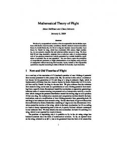
Figure A.1 – The flutter shutter gain function for the sinc-code (left). The Fourier transform (modulus) of the sinc − code (right), approximating the Fourier transform of the ideal gain function.

that the observed objects adopt a known (or learned) random velocity distribution. Analytical formulas are proposed that link an optimal flutter shutter code (see Fig. A.4) with the probability density of the expected motion blurs. Furthermore, in presence of random motions, an adequate flutter shutter is proved to significantly increase the expected SN R (beyond the bound of the first flutter shutter paradox), with respect to an optimal snapshot. Not only this theory permits to formalize the design of optimized codes given random velocity model. Conversely, it also allows us to analyze a posteriori any existing flutter shutter strategy, and to perform a reverse engineering of existing patented codes.

1

Related work

Blind deconvolution techniques [17, 18, 39, 61, 66, 71, 119] aim at estimating the blur and recovering the sharp image directly from the blurred one. Deconvolution algorithms have been developed intensively, [24, 48, 54, 95, 108, 123, 151]. For example in [154, 157] the authors suggest a modification of the Richardson-Lucy method [74, 104] to control the artifacts of the restored image. Other priors have been investigated in [59, 77, 159]. In [67] Fergus et al. use natural image statistics to estimate the blur. In [7, 8, 22, 27, 28, 32, 50, 51, 53, 56, 57, 60, 103, 116–118, 121, 122, 145, 149] good results are shown for the blur estimation and/or deblurring problem. Using the compressive sensing framework, the question of the order of the pair image estimation/motion estimation for deconvolution is addressed in [52]. Nevertheless, the power spectrum of images acquired with a blur of more than two pixels contains several zero crossings. Thus, useful information for image quality is irreversibly lost. Hence, no matter how sophisticated the image reconstruction is, it is virtually impossible to recover a de-blurred image without strong hypotheses on the underlying landscape. Such strong hypotheses are unrealistic for most images. The results are therefore in practice poor [111]. In an attempt to transform the blur problem into a well posed problem the authors of [19, 21, 23, 100] proposed to use two photographs with different blurs instead of one. In [136, 156] the authors use a long exposure image and another

5

Introduction

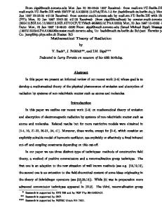
Figure A.2 – Sinc code : observed image (left). The blur interval length is equal to 52 pixels here. Reconstructed image (RM SE = 1.33) (middle). Residual noise (difference between ground truth and reconstructed, dynamic normalized on [0, 255] by an affine contrast change). The acquired image is “sharp”, it is no surprise since the sinc-code has a nearly constant Fourier transform thus, it does not alter any frequency.

one, sharp but noisy, to deblur the first. In [6] the authors suggest to take several images with several exposure times so that the blur in each image is different. If the zeroes of each Fourier transform do not coincide then it is possible to deblur by picking non zero coefficients in each image. In [124] a similar hybrid scheme is used where an image at high resolution and long exposure is taken simultaneously with a burst of low resolution and short exposure. In [10] a Mumford-Shah like variational model is proposed to simultaneously estimate the blur and deblur in presence of multiple objects motion from videos. In [110] the authors address the question of an automatic tuning of the exposure time to avoid overexposure in the case of still imaging. In [12] the authors treat the question of the optimal exposure time depending on the SN R of the restored image using a conventional camera. They consider the case of non invertible blurs with supports larger than two pixels, using a regularized deconvolution [33]. In [127] the authors use a full multi-image framework acquiring a bunch of sharp but noisy images and recovering a sharp image with increased SN R. For a review on multi image denoising the reader can refer to [15]. Conversely in [47] the authors reconstruct a movie from a single image using a temporally and spatially varying mask placed on the aperture. The mask helps encode the spatiotemporal information. In [35, 92, 125, 144, 150, 152] the authors use hybrid or complex camera systems. Unfortunately this kind of scheme may lead to other problems such as an expensive computational cost or hardware issues. The simplest hardware set up seems to be proposed in [3, 4, 6] by Agrawal et al. The new acquisition process modulates the photon flux into the camera by opening and closing the camera shutter according to certain well chosen pseudo random binary codes. In the case of a uniform motion in front of the camera, the resulting blur kernel becomes invertible (there are no zeroes in its Fourier transform), however big the velocity is. The visual result of an image acquired by flutter shutter is

6

I.1 Related work

5.5 5 4.5

RMSE

4 3.5 3 2.5 2 1.5 1 0

0.2

0.4

0.6

0.8

1

1.2

1.4

1.6

1.8

2

Blur support (pixel) Legend RMSE of snapshots (Boat image) RMSE of snapshots (House image) RMSE of snapshots (Alley image) RMSE of snapshots (Cameraman image) RMSE of snapshots (Peppers image)

Figure A.3 – This figure shows the RM SE curves for different snapshots kinds, on five test images (House, Alley, Boat, Cameraman, Peppers). On the x − axis, the blur support (|v|∆t) in pixels, on the y − axis the corresponding RM SE. The curves confirm that, on average, the blur support for a standard camera should be of approximatively ∆t∗ = 1.0909 pixel. A larger support would lead to a better SN R on the observed image samples, but the deconvolution would entail a lower SN R on the deconvolved image. The best snapshot is a compromise between the number of photons caught during a time span ∆t and the deconvolution kernel. It gives a reference to compare all flutter shutter strategies in terms of SN R.

close to a stroboscopic image, which can nonetheless give back a neat image by deconvolution. A compressive sensing flutter shutter camera was designed in [120] using random sequences where a blurry and low resolution image is acquired and processed to a neat and at high resolution image. Roughly speaking, the flutter shutter ensures that no information is lost by the motion blur; the compressed sensing technique deals with the increase of resolution. The compressed sensing technique is also used in [101] for spatio-temporal up-sampling. Alternatively the case of periodic events was investigated in [102]. In [63, 82, 90, 141] the authors use an active dynamic lighting pattern in place of the shutter to recreate a flutter shutter effect. The theory presented herewith works for this set up. In [79] the flutter shutter apparatus is applied to iris images and in [153] to bar-codes. In [78] the authors propose to optimize the binary flutter shutter code in function of the velocity of the scene. In [126] the authors use a local deblurring user-driven scheme on a flutter shutter embedded camera to deal with spatially varying blurs caused by the presence of several velocities in the observed scene. In [109] the authors treat the question of denoising an image taken by a flutter shutter camera, and also suggest an user assisted estimation of the blur. Their conclusion is that the denoising should be applied both

7

Introduction

1

1 0.9

0.8 Fourier tranforms (modulus)

0.8 0.7

Gain

0.6 0.5 0.4 0.3

0.6

0.4

0.2

0.2 0.1

0 -8

0 0

10

20

30 k

40

50

-6

-4

-2

60

0

2

4

6

8

4

6

8

xi Legend Fourier tranform (modulus) of the optimized flutter shutter gain function Ideal Fourier tranform (modulus)

Legend Flutter shutter code

1

1 0.9


0.8 0.7

Gain

0.6 0.5 0.4 0.3

0.6

0.4

0.2

0.2 0.1

0 -8

0 0

10

20

30 k


40

50

60

-6

-4

-2

0

2


Figure A.4 – Codes obtained assuming a truncated Gaussian density for the velocities. On the left from top to bottom: the code for a truncated Gaussian velocity distribution measured (x − axis k, y − axis gain αk ) using an increase exposure time factor of 5 and 10. This means that the first code has an exposure time five times greater than the best snapshot on average, the second 10 times. On pthe right the corresponding Fourier transform (modulus) of the code (see III.18) and the ideal Fourier transform 4 w(ξ) (VII.2) in bold. Those results permits to visualize the effect of the optimization. The conclusion is that nearly nop more improvement can be expected from the convergence of the computed αk coefficients of the code to the ideal 4 w(ξ) function. This is a consequence of Thm. 2.1 (chapter III).

before and after deconvolution. In [31] the authors treat the question of a posteriori motion estimation using a flutter shutter. In [40] a per pixel flutter shutter is used to build a camera that permits a post-capture balance between spatial and temporal resolutions of movies. A multi-camera equipped with flutter shutters is investigated in [2] and used to increase the frame rate of a single camera while having an increased amount of light captured compared to the equivalent hight-speed camera. A single camera equipped with a mask on the aperture and an array of light sources is used in [65] to construct the visual hull of an object (shape from silhouette). Another solution to get an invertible motion blur using only one image was found in [69] where Levin et al. suggested to move the camera in the direction of the motion during the exposure time. The authors use a constant acceleration motion in order to make the resulting kernel invertible and spatially invariant to the velocity. Hence an a priori knowledge of the motion direction is required. This approach has been generalized in [25] to the case of unknown directions, but it uses two images instead of one. In [81] the motion-invariant photography apparatus is implemented using the lens of the camera. In any cases, these approaches cause blur in static parts of the scene. Yet, thanks to the invertibility (well-posedness of the recovery problem),

8

I.2 Overview

in both cases, the sharp image can be recovered by a deconvolution. Notice that only one image is acquired and recovered at the end of the process. Alternatively in [9, 36, 68, 72, 76, 84, 88, 143] authors use a temporally fixed and spatially varying mask in order to estimate the depth, and/or refocus the out of focus part to get an always in focus (neat) image. In [45] the authors deal with the question of the optimal tradeoff between depth of field and exposure time. In [38] the authors take advantage of CMOS imaging sensors to implement a coded rolling shutter to trade vertical resolution for an increased dynamic range. The authors of [140] also suggest to use a camera equipped with a mask on the aperture camera and to take purposely out of focus images with a mask to increase the dynamic range. Their conclusion is rather negative “None of the possible combinations of aperture filter and deconvolution algorithm were able to consistently reduce the dynamic range of the captured image without excessively degrading image quality”. Another computational camera is designed in [86] where the aperture is equipped with a mask and the sensor is moved at a constant velocity during the exposure. It is used to control the depth of field, create bokeh or a depth invariant blur size. Another camera prototype was designed in [73], where the authors suggest a programmable aperture (mask). It is also used for depth and digital refocusing. An interesting implementation, the Frankencamera, was proposed in [1]. It permits to “control and synchronization of the sensor and image processing pipeline at the microsecond time scale, as well as the ability to incorporate and synchronize external hardware like lenses and flashes”. The authors demonstrate six computational photography applications. An even more complex scheme involving a fixed mask close to the sensor and dynamic one on the aperture is investigated in [5], where the authors explore the feasibility of post processing trade offs between spatial, angular and temporal resolutions. Finally reviews of computational photography can be found in [75, 96, 97, 161].

2

Overview

This thesis focuses on the various set ups permitting to acquire an image degraded by an invertible motion blur, namely the Agrawal et al. flutter shutter and the Levin et al. motion-invariant photography. Chapter II section 1 proposes a general mathematical framework for image acquisition using a physical Poisson model for the photons capture process, including the obscurity noise. This model suits well our context since all noise terms inherent to image sensing are taken into account without any approximation. The model is detailed in a static context in section 2. Fourier-based SN R definitions are given in section 4, to take into account the deconvolution later on. The model is applied to the still photography in section 5. The non stationarity motion induced case is introduced in section 6 and the multi-images fusion is discussed in section 7. In chapter III the mathematical model of chapter II is used to analyze the numerical flutter shutter, a digital implementation of the classic flutter shutter method. This set up is the most flexible, adaptive to all motion and allows for negative gains. The numerical flutter shutter does not reduce the number

9

Introduction

of photons caught by the sensor and it is proven later on that it yields the best possible SN R. It is proven that it actually works and, for any flutter shutter gain function a formula providing the SN R of the neat deconvolved image is given. The numerical flutter shutter gain function is in principle piecewise constant nevertheless, it is useful for the theory to extend it to continuous gain functions. In section 2 a reverse formula permits to get back an equivalent piecewise constant numerical flutter shutter. Chapter IV investigates classic analog implementation of the flutter shutter. This analog flutter shutter is a generalization of the original Agrawal et al. flutter shutter which allows for smoother, non binary, gain functions. For any analog flutter shutter apparatus, an explicit formula to measure directly the SN R of the deconvolved sharp image is given. Section 2 proves that the numerical flutter shutter SN R is always larger than the analog flutter shutter SN R with the same gain function. A snapshot theory is developed in chapter V section 1. The standard camera apparatus is explored as a particular flutter shutter strategy. The SN R of the deconvolved image is calculated, for any standard acquisition strategy. The standard camera is optimized to get the best SN R possible, taking the deconvolution into account. This yields a precise definition of the best possible snapshot in presence of known motion. This best snapshot is used later on as a reference in terms of SN R. In section 2 the Levin et al. motion-invariant photography is proven to be a particular case of the general analog flutter shutter theory. The SN R of the motion-invariant photography apparatus is computed and compared with the other flutter shutter strategies. This section also proposes to implement the motion-invariant photography kernel using a numerical flutter shutter. This permits to generalize the motion-invariant photography method to the case where the direction of the relative velocity v is not a priori known. Chapter VI proves that the use of any flutter shutter does not increase indefinitely the SN R of the sharp recovered image. It is proven that the best flutter shutter entails a 17% increase of the SN R compared to the best snapshot. It is also proven that, even though the exposure time remains unchanged, the flutter shutter does beat the standard camera with classic aperture. These two results are the flutter shutter paradoxes. Chapter VII proposes a solution to the first flutter shutter paradox theorem provided the probability density of the observed velocities is known. Section 1 gives analytical formulae that link an optimal flutter shutter code with any probability density of the expected velocities. A backward analysis, computing the probability density of any (patented) code is given in section 2. This framework is also applied to the standard camera in section 3. All results are illustrated in chapter VIII. Section 1 shows simulations of several flutter shutter strategies, including the Agrawal et al. flutter shutter code and the Levin et al. motion-invariant photography. A reverse engineering of classic flutter shutter codes is performed in section 2. Section 3 provides optimized codes and comparisons with the best snapshot on average, for centered-Gaussian, uniform (with different sdt-dev σ and ranges) and an handcrafted distribution of the velocity.

10

Chapter II Still Photography Theory Abstract : This chapter starts by modeling the stochastic photon capture by a light sensor, given that the photon flux is a Poisson space-dependent emission. It takes into account both the classic shot noise and the obscurity noise. To cope with the fact that the image noise is colored after deconvolution, a “spectral” definition is used for the signal to noise ratio (SN R). The SN R is computed without approximation, from the proposed model. The modeling will treat in the same formalism all possible types of flutter shutter, including an analog model, a digital model, the classic Agrawal et al. flutter shutter, and the Levin et al. motion-invariant photography.

1

Mathematical modeling

This section presents a continuous stochastic model of photons captured by a sensor array. The model applies to a standard image acquisition on still or moving landscapes, provided the motion is uniform and stationary. Without loss of generality (w.l.o.g.) the formalization will be done in the case where the sensor array is 1D and the landscape moves in the direction given by the sensor. Let Pl : ❘+ × ❘ be a bi-dimensional Poisson process of intensity l(t, x), ∀(t, x) ∈ ❘+ × ❘ (here l is

called landscape, t and x are the time and spatial positions, respectively). This means that for every a, b, t1 , t2 (with a < b and 0 ≤ t1 < t2 ) Pl ([t1 , t2 ] × [a, b]) is a Poisson random variable with intensity R t2 R b t1

a

l(t, x)dxdt. The theoretical observation of a pixel sensor (photon counter) of unit length centered

at x during the time span [0, ∆t] is a Poisson random variable Pl

1 1 [0, ∆t] × [x − , x + ] ∼ P 2 2

Z ∆t Z x+ 1 2 0

x− 21

l(t, y)dydt

!

where [x − 21 , x + 21 ] represents the normalized sensor unit, and X ∼ P means that a random variable

X has law P . In other terms the probability to observe k photons coming from the landscape l seen

11

Chapter II. Still Photography Theory

at the position x on the time interval [0, ∆t] and using a normalized sensor is

P Pl

2

1 1 [0, ∆t] × [x − , x + ] = k = 2 2

R ∆t R x+ 12 x− 21

0

l(t, y)dydt

k − R ∆t R x+ 21 l(t,y)dydt 1 0 x− 2

e

k!

.

The still photography case

In the classic still photography set up, l(t, x) = l(x), which makes of Pl : ❘+ × ❘ a bi-dimensional

time stationary and spatially inhomogeneous Poisson process of intensity l(x), ∀(t, x) ∈ ❘+ × ❘. Thus

for every a, b, t1 , t2 (s.t a < b and 0 ≤ t1 < t2 ) Pl ([t1 , t2 ] × [a, b]) is a Poisson random variable with

intensity

R t2 R b t1

a

l(x)dxdt = |t2 − t1 |

Rb a

l(x)dx (by stationarity of the process).

Then the theoretical observation of a pixel sensor (photon counter) of unit length centered at x using an exposure time of ∆t is a Poisson random variable Pl

1 1 [0, ∆t] × [x − , x + ] ∼ P 2 2

Z ∆t Z x+ 1 2 x− 12

0

l(y)dydt

!

∼ P ∆t(✶[− 1 , 1 ] ∗ l)(x) 2 2

where ∆t is the exposure time, using a normalized sensor of unit length, and ∗ denotes the convolution

(viii). (Here and in the rest of the text, Latin numerals refer to the formulas in the final glossary page ix.) For sampling purposes we assume that the theoretical landscape l is seen through an optical system with a point spread function g. Definition We call ideal landscape the deterministic function u = ✶[− 1 , 1 ] ∗ g ∗ l

(II.1)

2 2

where g is the point spread function of the optical system providing a cut off frequency. In other words, thanks to the convolution with g the acquisition system is able to sample u. From the imaging point of view if the center of the pixel sensor is x then u(x) represents the ideal (noiseless) pixel landscape value, which unfortunately can only be obtained after infinite exposure time. Definition (Ideal acquisition system.) The image acquired by the ideal acquisition system, before sampling, corresponds to samples of the Poisson process Pl . The intensity u (ideal landscape value) is related to the landscape l by (II.1) and is band limited. 1 1 Pl ([t1 , t2 ] × [x − , x + ]) ∼ P 2 2

12

Z t2 t1

u(x)dt ∼ P (|t2 − t1 |u(x)) .

(II.2)

II.3 Sampling, interpolation

Definition (Real acquisition system with noise included in the landscape.) A more realistic acquisition system adds a landscape independent noise also known as dark noise (or obscurity noise or thermal noise). Assuming that this noise has variance η (II.2) entails 1 1 Pl+η ([t1 , t2 ] × [x − , x + ])) ∼ P (|t2 − t1 |(u(x) + η)) . 2 2

(II.3)

Independently of their thermal cause, thermal photon emission is Poissonian. Furthermore, at each pixel sensor the number of thermal photons caught is independent of the number of photons caught coming from the landscape u. Therefore, the sum of the numbers of thermal and landscape photons hitting the sensor is a Poisson random variable whose intensity is the sum of the thermal and landscape intensities. Hence, all computations using the "noisy" landscape u + η remain formally the same as with the noiseless ideal acquisition system defined in (II.2). The estimator considered is unbiased. Nevertheless this means that, in the sequel u + η is estimated, not u. However, notice that u and u + η only differ by a constant which only affects the mean of the image and does not change the perceptual quality. As a matter of fact it only impacts the null frequency of the SN R function as it is defined by Boracchi et al. in [12] and does not change the ‘spectral-averaged” SN R of section 4 compared to estimating u. Therefore, w.l.o.g. we will assume that u already contains the obscurity noise in itself. Notice that η being a constant, u + η and u have the same cut off frequency. We will also always assume in the sequel that u ∈ L1 ∩ L2 (❘). This assumption will be necessary to apply some of

the mathematical formulas, but represents no artificial restriction on the acquisition physical model. Indeed, first, the average photon emission is always bounded. Second, taking a large enough support, we can always suppose w.l.o.g. that the landscape has bounded support and that the acquisition time is large but not infinite. Thus we can assume that the noise is zero at infinity. Under these conditions u ∈ L1 ∩ L2 .

3

Sampling, interpolation

In the following the landscape u is assumed band limited, namely u ˆ (see the definition (xxiv) of Fourier transform in the glossary) is supported in [−π, π] and therefore can be sampled at a unit rate. This hypothesis is again no restriction, being justified by the frequency cutoff provided by the optical kernel g. The discrete sensor observations, or samples, will be denoted by e(n) for n ∈

a very long exposure T of a static scene, by the law of large numbers we have u(n) = ❊e(n).)

e(n) T

❩. (Under

→ u(n), and

Definition Given a discrete array observation e(n), n ∈ ❩, its band limited interpolate e(x) for x ∈ ❘

can be defined by Shannon-Whittaker interpolation as e(x) =

X

n∈❩

e(n)sinc(x − n)

( see in (xxix) the definition of sinc.)

(II.4)

13


Notice that in the deterministic ideal case, e(n) = u(n) and, u being band-limited, we would deduce e(x) = u(x) from e(n) = u(n). By (II.4) we also have eˆ(ξ) =

4

X

n∈❩

e(n)e−inξ ✶[−π,π] (ξ).

(II.5)

Noise measurement

Definition In the following we call signal to noise ratio (SN R) of a random variable X the ratio

For example if

SN R(X) := p

|❊X| . var(X)

(II.6)

✉est (x) (resp. ✉ˆ est (ξ)) is an estimation of the landscape u(x) (resp.

u ˆ(ξ)) based on a

noisy observation of u, SN R(✉est (x)) := p

Likewise, we call “spectral SN R” of

|❊✉est (x)| . var(✉est (x))

(II.7)

✉est the frequency dependent ratio defined by

SN Rspectral (ˆ ✉est (ξ)) := p

|❊✉ ˆ est (ξ)| (var(ˆ ✉est (ξ))

for ξ ∈ [−π, π]

(II.8)

and introduced by Boracchi et al. in [12]. We call “spectral-averaged” SN R the ratio defined by SN R

spectral−averaged

(ˆ ✉est ) :=

1 R 2π q R 1 2π

|❊✉ ˆ est (ξ)|✶[−π,π] (ξ)dξ

var(ˆ ✉est (ξ)✶[−π,π] (ξ))dξ

.

(II.9)

Lets show first that this definition makes sense. In the sequel, the considered estimator is unbiased. This implies that ❊✉ ˆ est (ξ) = ✉ ˆ (ξ). Furthermore, since u ∈ L1 (❘) by Riemann-Lebesgue’s we get that

u ˆ(ξ) is continuous, so is |❊✉ ˆ est (ξ)| = |ˆ ✉(ξ)|. Hence |❊✉ˆ est (ξ)| is integrable on the interval [−π, π]. The R variance term var(ˆ ✉est (ξ)✶[−π,π] (ξ)) is positive. Thus, var(ˆ✉est (ξ)✶[−π,π] (ξ))dξ converge in ❘¯ + . It would be infinite if some frequency interval is lost and, in this case the SN Rspectral−averaged (ˆ ✉est ) = 0.

This means that the above definition is correct, at least in a mathematical sense. Now, lets turn to its meaning. Proposition 4.1. Given ✉ ˆ est (ξ) an unbiased estimator of u ˆ(ξ) then SN Rspectral−averaged (ˆ ✉est ) =

C . RM SE(u, uest )

Proof. The mean squared error (M SE) can be decomposed into bias and variance terms. Since the estimator is unbiased the bias term is zero. Its variance term is equal to

14

R

var(✉est (ξ))dξ =

II.5 Standard acquisition, the SN R with no blur

R

❊|✉est (ξ)|2 dξ + |❊✉est (ξ)|2 dξ. Furthermore, on one hand we have Z

R

❊|ˆ ✉est (ξ)✶[−π,π] (ξ)| dξ = ❊ 2

Z

= 2π ❊

|ˆ ✉est (ξ)✶[−π,π] (ξ)| dξ

Z

2

|✉est (x)|2 dx = 2π

Z

(by Fubini for positive functions)

❊|✉est (x)|2 dx (by Fubini, again).

On the other hand, we have Z

|❊✉ ˆ est (ξ)✶[−π,π] (ξ)|2 dξ =

Z

|ˆ u(ξ)✶[−π,π] (ξ)|2 dξ (unbiased estimator)

= 2π

Z

2

|u(x)| dx = 2π

Z

|❊✉est (x)|2 dx.

Consequently, SN R

spectral−averaged

(ˆ ✉est ) =

1 2π

R

|❊✉ ˆ est (ξ)|✶[−π,π] (ξ)dξ

qR

var(✉est (x))dx

=

Constant . RM SE(u, uest )

Notice that, the naive average of the SN R function defined in [12], would not reflect the RM SE. Worse, it would not vanish if some frequency interval is lost. Such information loss implies that the flutter shutter is not invertible. The invertibility of the flutter shutter is discussed and the inverse filter is defined page 25. The reason of these definitions is to compare in terms of SN R the flutter shutter method to a standard “quick enough to be sharp" snapshot image acquisition strategy in the sense of (II.6), (II.7), (II.8), (II.9).

5

Standard acquisition, the SN R with no blur

From the acquisition system definition (II.3) the observed image at position x using the standard image acquisition strategy with an exposure time L∆t can be any realization of 1 1 Pl ([0, L∆t] × [x − , x + ]) ∼ P 2 2

Z

u(x)dt

[0,L∆t]

!

∼ P (L∆tu(x)) .

(II.10)

Notice that in this case the expected value and variance of a pixel sensor at position x are equal to L∆tu(x). Theorem 5.1. (Fundamental theorem of photography) In the case of a still image, the SN R satisfies SN R(x) =

p

u(x)L∆t, where L∆t is the total exposure

time. It is therefore proportional to the square root of both the exposure time and the light intensity. Remark In a passive optical system we have no control over the landscape light emission u(x). No

15


lighting is possible, to boost the photon emission. Thus the only secure way to increase the SN R is to increase the exposure time L∆t. Proof. Let entails

✉est ∼

Pl ([0,L∆t]×[x− 12 ,x+ 12 ]) L∆t

be the estimate of the ideal landscape u. The relation (II.10)

✉est (x) ∼ Then ❊(✉est (x)) = u(x) and

✉est (x) is an unbiased estimator for u(x). var(✉est (x)) =

It follows from (II.7) that SN R(✉est )(x) =

6

P (L∆tu(x)) . L∆t The variance of

✉est (x) is

L∆tu(x) u(x) = . 2 (L∆t) L∆t

p

u(x)L∆t.

Image acquisition with a moving landscape

In the following the camera focal plane is always taken as reference plane. The camera is always assumed to move parallel to its focal plane in a straight trajectory in the x direction (Fig. A.1). Hence the acquisition process is made in the x direction only. The camera moves straight at a speed v(t) (counted in pixels per second) and the landscape is static. These assumptions may seem simplistic, but are actually technologically relevant, as they include the scanning of planar scenes like documents, or of scenes seen at a long distance, like aerial video and push broom satellites. Thus from now on we assume l(t, x) = l(x − tv(t)), and mainly v(t) ≡ v where l is the underlying

stationary landscape model (section 2). Hence all the former discussion made on the acquisition system, sampling and interpolation holds. This section focuses on the mathematical model for standard photography, where there is either a motion blur in a single continuous exposure, or the acquisition of an image burst (several consecutive snapshots with shorter exposure). We shall give the conditions under which the exposure is short enough to get a quality photograph, and evaluate the SN R in all three cases: snapshots, longer exposure with motion blur, and image burst made of short enough snapshots.

6.1

Standard motion blur

In the following we fix an exposure time unit ∆t, and measure exposure times as its multiples L∆t. Theorem 6.1. The standard motion blur is equivalent to an image obtained by a convolution of the ideal landscape u by a fixed (window shaped) kernel ✶[0,b] where b is the blur length, equal to Lv∆t. Proof. The ideal landscape u is moving in the camera frame at a speed v (counted in pixels per second)

16

II.6 Image acquisition with a moving landscape

Figure A.1 – Acquisition system: the camera plane moves parallel to the focal plane in fixed direction, with scalar speed v(t). x − axis : position, y − axis : intensity of photon emission by the landscape at position x. The exposure time L∆t is assumed short enough, or the camera elevation large enough to ensure that there is no apparent deformation of the landscape due to its varying height.

and using (II.3) we get that the acquired image at position x can be any realization of 1 1 Pl ([0, L∆t] × [x − , x + ]) ∼ P 2 2

Z L∆t 0

u(x − vt)dt

!

1 ∼ P ( ✶[0,Lv∆t] ∗ u)(x) . v

In this case the expected value and variance of a pixel sensor at position x are equal to v1 (✶[0,Lv∆t] ∗

u)(x). The quantity Lv∆t is nothing but the length of the blur b (in pixels).

Remark The convolution with h = ✶[0,Lv∆t] (standard blur) function is a non-invertible transformation as soon as the first zero of the Fourier transform (FT) of h is in the support of u ˆ. This makes ill posed any restoration process of u. The purpose of the flutter shutter method will be to replace

✶[0,Lv∆t] with a function whose convolution remains invertible for arbitrary Lv∆t = b. If instead, as ˆ is outside the support of u considered in the next paragraph, the first zero of h ˆ, then the motion blur

17


is said negligible and it is actually invertible.

7

The multi-image fusion to improve the SN R

The multi-image acquisition strategy consists in taking a burst of L images using a ∆t exposure time. The exposure time ∆t is taken small enough, so that the elementary blur of each one of the L images is negligible (see chapter III section 1.3). Each image is registered and added to the former ones to obtain a single accumulated image. See [15] for an analysis of the feasibility of this technique. We shall assume here that the registration operation is error-free, so that the operation amounts to an increased exposure time with a stationary landscape. Theorem 7.1. The multi-image acquisition strategy using L images increases the SN R by a factor √ of L compared to a standard snapshot. Proof. Before the registration operation the k-th image observed (for k ∈ {0, L − 1}) at position x is (a realization of)

1 1 Pl ([k∆t, (k + 1)∆t] × [x − , x + ]) ∼ P 2 2

Z ∆t 0

u(x − vk∆t − vt)dt

!

1 (✶ ∗ u)(x − vk∆t) . ∼P v [0,v∆t] The registration operation consists in a perfect translation τ (x) = x + vk∆t of the previous observed, hence simulating a stationary landscape. After the registration operation the k-th image observed for k ∈ {0, L − 1} at position x is (a realization of) P

1 (✶ ∗ u)(x) . v [0,v∆t]

Finally the image is constructed by adding all observations, so it is (a realization of) L−1 X

1 1 (✶[0,v∆t] ∗ u)(x) ∼ P L (✶[0,v∆t] ∗ u)(x) . P v v k=0

(II.11)

(This last equivalence uses the independence of the Poisson random variables, justified by the disjoint time intervals). Following the same scheme used in (Thm. 1.1) from (II.11) we get the estimated uest,mul

v 1 ∼ P L (✶[0,v∆t] ∗ u)(x) L v

whose variance is L times smaller. Thus the L factor remains in all equations. Finally from (V.1, V.6) √ we deduce that the SN R is increased by a L factor.

18

II.7 The multi-image fusion to improve the SN R

In other words the use of a multi-image fusion with a sufficient L permits to achieve any SN R. This result will contrast with the first flutter shutter paradox that an infinite time exposure does not grant an infinite SN R. This is the object of the next chapters.

19


20

Chapter III The Numerical Flutter Shutter Abstract : This chapter defines a digital implementation of the flutter shutter compatible with recent technologies. This set up is the most flexible, adaptive to all motion and allows for negative gains. Furthermore, the numerical flutter shutter does not reduce the number of photons caught by the sensor and it is proven later on that it yields the best possible SN R. It is investigated using the model of photon acquisition of chapter II. A closed formula is obtained giving explicitly the SN R of the sharp deconvolved image. The numerical flutter shutter gain function is in principle piecewise constant. Nevertheless, it is useful for the theory to extend it to continuous gain functions. Anyway, a reverse formula permits to get back an equivalent piecewise constant numerical flutter shutter from any continuous gain function. After having treated the classic image acquisition strategies, we are now in a position to treat the various flutter shutter strategies and to compare them to the classic ones. Two things are at stake: first, to prove that the various flutter shutters actually work, and second to evaluate the SN R of the resulting image and to compare it to the SN R of classic strategies. The hope would be that the flutter shutter retains the very interesting feature of the multi image denoising, namely an increase of the √ SN R by a factor proportional to L∆t, the total exposure time. We shall see that this is not so.

1

The numerical flutter shutter

The numerical flutter shutter method consists in a numerical sensor gain modification taking place after the acquisition by the sensor. Roughly speaking the camera takes a burst of L images using an exposure time ∆t. The k-th image is multiplied, for k ∈ 0, ..., L − 1, by an αk ∈

❘

gain. Then all

images are added to obtain one observed image, the flutter shutter. The exposure time ∆t must be small enough so the blur of each image is negligible (definition in chapter V section 1). This technique is similar to the multi-image acquisition strategy but does not use any registration technique. According to, for example, [64, 89] an image sensor can have a duty ratio of nearly 100% (the duty ratio is the ratio of light integration time over readout, storage, reset times - that is the percentage of useful time). It means that a sensor can integrate light without interruption. Thus, the numerical flutter shutter,

21

Chapter III. The Numerical Flutter Shutter

as it is described below without “dead time” between two consecutive gains ak is perfectly reasonable from a technological viewpoint. Nevertheless, it seems that its interest is limited: why not keeping all images instead of adding them all? One of the obvious reasons is compression, particularly for Earth observation satellites. In that case the motion blur due to a drift in satellite trajectory estimate could be eliminated by a flutter shutter, without any additional transmission (or computational) burden if only the flutter shutter image (the sum) is transmitted. The k-th acquired elementary image at a pixel at position n is a realization of P

Z (k+1)∆t k∆t

!

u(n − vt)dt .

The flutter shutter observation is obtained by combining the k-th output with weight αk . Thus the flutter shutter output at a pixel centered at n is obs(n) ∼

L−1 X

αk P

k=0

Z (k+1)∆t k∆t

u(n − vt)dt

!

(III.1)

where by construction obs(n) are obtained for n ∈ ❩ and are independent. Indeed, the sensors are

disjoint and do not receive the same photons. In the following it will be useful to associate with the flutter shutter its code defined as the vector (αk )k=0,··· ,L−1 , and its flutter shutter function defined by α(t) = αk for t ∈ [k∆t, (k + 1)∆t[. Definition Let (α0 , ..., αL−1 ) ∈ ❘L be a flutter shutter code. We call numerical flutter shutter samples at position n of the landscape u at velocity v the random variable obs(n) ∼

L−1 X

Z (k+1)∆t

αk P

k∆t

k=0

!

u(n − vt)dt .

(III.2)

We call numerical flutter shutter its band limited interpolate obs(x) ∼

X

n∈❩

obs(n)sinc(x − n).

We call flutter shutter function the function α(t) =

L−1 X

αk ✶[k∆t,(k+1)∆t[ (t).

(III.3)

k=0

Remark It is good to keep in mind the following trivial and less trivial examples: 1. αk = 1 ∀k ∈ {0, ..., L − 1} (pure accumulation prone to motion blur) 2. αk = 0 or 1 ∀k ∈ {1, ..., L − 1} with form)

22

P

αk =

L 2

(Agrawal et al.’s flutter shutter has this generic

III.1 The numerical flutter shutter

3. α0 = 1 and αk = 0 ∀k ∈ {1, ..., L − 1} (standard snapshot)

1.1

The motionless case v = 0

We shall first consider the ideal motionless case where v = 0. In this situation the acquired image has simply lost some photons with respect to an accumulation image, because some of the αk are null. Thus in the motionless case, the flutter shutter cannot but decrease the SN R. This is easily confirmed by the following calculation. We have obs(x) ∼

L−1 X

αk P (∆tu(x)) .

k=0

Thus

❊ (obs(x)) =

L−1 X

αk ∆tu(x)

(III.4)

k=0

and var (obs(x)) =

L−1 X

αk2 ∆tu(x).

(III.5)

k=0

From (III.4) we deduce that the estimated landscape

✉est is obtained using

obs(x) . k=0 αk ∆t

✉est (x) ∼ PL−1

(III.6)

Let r ∼ ✉est − u be the residual error then from (III.4-III.5) we get

❊(r(x)) =

❊ (obs(x)) PL−1 k=0

αk ∆t

− u(x) = 0.

Hence F(✉est ) is an unbiased estimator for u ˆ. Moreover, from (III.5, III.6) we deduce P

P

u(x) L−1 α2 u(x) L−1 α2 var (obs(x)) = PL−1 k=0 k = PL−1 k=0 k . var (r(x)) = PL−1 ( k=0 αk )2 ∆t2 ( k=0 αk )2 ∆t ( k=0 αk )2 ∆t Thus, by (II.7), SN R(✉est ) = x 7→

x2

s

PL−1 α k )2 u(x)∆t Pk=0 L−1 2 . Since by Jensen’s inequality applied to the convex

function we always have

(

k=0

αk

1 PL−1 2 L ( k=0 αk )

≤

PL−1 2 k=0 αk , the (numerical) flutter shutter is less

favorable than a mere accumulation. To give an example, in the case of r a Agrawal et al.qcode where 2 u(x)∆tL , to αk = 0 or 1 and the number of non null αk is L/2. Then the SN R is u(x)∆t (L/2) 2 L/2 =

be compared to the pure accumulation case where αk = 1 and the SN R is

q

2

u(x)∆t LL =

p

u(x)∆tL.

23


Thus the Agrawal et al. flutter shutter entails in the motionless case a

√

2 loss factor for the SN R.

We now pass to the general more interesting case, namely when there is a motion.

1.2

Flutter shutter in presence of motion

Theorem 1.1. The observed samples of the numerical flutter shutter are such that, for n ∈ ❩

❊ (obs(n)) =

. 1 α v v

var(obs(n)) =

1 2 . α v v

∗ u (n)

(III.7)

and

∗ u (n).

(III.8)

Proof. From the numerical flutter shutter samples definition (III.2),

❊ (obs(x)) =

L−1 X

αk

k=0

Z (k+1)∆t k∆t

u(x − vt)dt =

Z L∆t 0

α(s)u(x − vs)ds

(III.9)

where we recall that α=

L−1 X

αk ✶[k∆t,(k+1)∆t[ .

k=0

Thus,

❊ (obs(x)) =

Z Lv∆t 1

y α( )u(x − y)dy = v v

0

1 . α v v

∗ u (x).

(III.10)

Similarly from (III.1) var(obs(x)) =

L−1 X k=0

αk2

Z (k+1)∆t k∆t

u(x − vt)dt =

1 2 . α v v

∗ u (x).

Notice that obs(x) is not necessarily a Poisson random variable. However, if all αk are equal to 0 or 1 then by (III.9) obs(x) ∼ P

1 . α v v

∗ u (x),

because we are adding independent Poisson random variables. On the other hand, if for some k, αk 6∈ {0, 1}, then if X ∼ P(λ) then αk X is not a Poisson random variable.

24


Ideal numerical flutter shutter The formulas of Theorem 1.1 giving the samples obtained by flutter shutter appear not to depend on the particular form of α as a piecewise constant function on a finite set of intervals with length ∆t. As a matter of fact, we can envisage any function α ∈ L2 (❘) to be numerical flutter shutter, for an

ideally controlled camera where at each instant the gain α(t) is changed. This leads to the following definition and corollary. Corollary 1.2. We call continuous numerical flutter shutter any band-limited and bounded gain function α ∈ L2 (❘). Then the formulas (III.7) and (III.8) of Theorem 1.1 are still valid.

Proof. By assumption the observed ideal landscape u belongs to L1 ∩L2 (❘). We recall that L1 ∗L2 ⊂ L2

and L2 ∩ L2 ⊂ C0 (❘) (the set of continuous functions on ❘ tending to 0 at infinity). Furthermore,

α being band limited is continuous. Being also bounded, the expectation and variance functions of (III.7) and (III.8) are continuous and therefore well defined at any point. It remains to show that

these formulas are valid for a general gain function. Consider for this an approximation of α(t) by a finite numerical flutter shutter code (αk )k such that (αk )k tends to α in L1 , L2 and L∞ , (that is, uniformly) when k → ∞. The formulas (III.7) and (III.8) are valid for (αk )k , and the corresponding

formulas for α are deduced by passing to the limit.

From now on, unless specified otherwise, by numerical flutter shutter, and by α we shall mean a continuous numerical flutter shutter.

1.3

The inverse filter of a numerical flutter shutter

Step 1: the noiseless case

. 1 vα v

Let us examine first the discrete noiseless case, when obs(n) =

∗ u (n) and obs(n) is obtained for n ∈ ❩ but being band limited, can be interpolated to

obs(x), for any x ∈ ❘. Then

. 1 α F v v

∗ u (ξ) = u ˆ(ξ)ˆ α(ξv).

ˆ(ξ) = 0 for |ξ| > π. Hence for the By hypothesis (see chapter II section 2) we assumed that u

invertibility we must only require that |ˆ α(ξv)| > 0 for ξ ∈ [−π, π].

Definition We say that a flutter shutter α is invertible (for velocities |v| smaller than |v0 |) if |ˆ α(ξ)| > 0

for ξ ∈ [−π|v0 |, π|v0 |].

If the flutter shutter is invertible, we can consider the inverse filter γ defined by γˆ (ξ) =

✶[−π,π] (ξ) α ˆ (ξv)

.

(III.11)

25


Since α ∈ L1 (❘), ξ 7→ α ˆ (ξ) is bounded and continuous. If α(ξv) ˆ is nonzero on [−π, π], γˆ will therefore

be bounded and supported on [−π, π]. In consequence, under this assumption, γ is C ∞ , bounded, and band-limited. We shall as logical define the recovered landscape from noisy data by the formulae that would be valid for noiseless data. Assume that we observe e(n) = ❊(obs(n)) for n ∈ ❩ and wish to compute

eˆ(ξ) from the discrete observed (e(n))n∈❩ . Since e(x) is band limited, we can interpolate it using the band limited interpolation (II.4). The band limited interpolate of the ideal observation is X

e(x) =

e(n)sinc(x − n).

(III.12)

e(n)e−inξ ✶[−π,π] (ξ).

(III.13)

n∈❩

Then from (III.12) we have eˆ(ξ) =

X

n∈❩

So the ideal deconvolved landscape d(x) obtained by combining (III.11) and (III.13) is ˆ = d(ξ)

−inξ ✶ [−π,π] (ξ) n∈❩ e(n)e

P

α ˆ (ξv)

.

(III.14)

We shall now adopt the same formulae for the noisy case.

Flutter shutter landscape recovery in the real noisy case

Definition Assume that a flutter shutter with code α is invertible. We call estimated landscape

✉est,num of the numerical

flutter shutter the function defined by F(✉est,num )(ξ) =

−inξ ✶ [−π,π] (ξ) n∈❩ obs(n)e

P

α ˆ (ξv)

,

where the observed obs(n) samples (III.1) are used instead of the ideal e(n) in (III.14). Theorem 1.3. The numerical flutter shutter has a spectral SN R (II.8) equal to |ˆ u(ξ)||ˆ α(ξv)| ; SN R(ξ) = ✶[−π,π] (ξ) p ||u||L1 ||α||L2

the expected value of the estimated landscape F(✉est,num )(ξ) from the observed samples is

❊(F(✉est,num )(ξ))) = uˆ(ξ)✶[−π,π] (ξ);

26

(III.15)


and its variance is var(F(✉est,num (ξ))) =

||α||2L2 ||u||L1 ✶[−π,π](ξ) . |ˆ α(ξv)|2

(III.16)

Proof. By (III.8, III.15), var(F(✉est,num )(ξ)) =

var

P


|ˆ α(ξv)|2 −inξ ✶ 2 [−π,π] (ξ)| n∈❩ var(obs(n))|e |ˆ α(ξv)|2

=

P

=

P

n∈❩

1 2 vα

. v

∗ u (n)✶[−π,π](ξ)

|ˆ α(ξv)|2 ∗ u||L1 ✶[−π,π](ξ) = |ˆ α(ξv)|2 2 1 1 . . 2 v ||α v ||L1 ||u||L1 ✶[−π,π](ξ) v ||α v ||L2 ||u||L1 ✶[−π,π](ξ) = = |ˆ α(ξv)|2 |ˆ α(ξv)|2 v 2 2 ||α||L2 ||u||L1 ✶[−π,π](ξ) ||α||L2 ||u||L1 ✶[−π,π](ξ) = v = . |ˆ α(ξv)|2 |ˆ α(ξv)|2 || v1 α2

. v

(III.17)

In this proof the crucial point is the use of the Poisson summation formula (xxx) in equation (III.17). Following the same scheme and starting from (Thm. III.7) ❊(F(✉est,num (ξ))(ξ) can be computed by using (for the derivation of the third line) the second Poisson formula (xxx), and the fact that u is band limited with u ˆ supported on [−π, π]:

❊(F(✉est,num (ξ))) =

❊

P

=

P

=

P

n∈❩

F = =


α ˆ (ξv)

1 . vα v

m∈❩ F

1 . vα v

1 . vα v

∗ u (n)e−inξ ✶[−π,π] (ξ) α ˆ (ξv)

∗ u (ξ + 2πm)✶[−π,π](ξ) α ˆ (ξv)

∗ u (ξ)✶[−π,π](ξ) α ˆ (ξv)

v ˆ (ξv)ˆ u(ξ)✶[−π,π](ξ) vα

α ˆ (ξv)

=u ˆ(ξ)✶[−π,π] (ξ).

27


From (III.16) and using the definition of the spectral SN R (II.8), we obtain |ˆ u(ξ)||ˆ α(ξv)| . SN Rspectral (✉est,num (ξ)) = ✶[−π,π] (ξ) p ||u||L1 ||α||L2 Remark From (III.16) we also deduce that var(F(✉est,num )(ξ)) is invariant by changing α into λα for λ 6= 0 (rescaling): as could be expected, the flutter shutter code is defined up to a multiplicative

constant.

Remark Going back to the case where α is a discrete numerical flutter shutter, we can see a necessary condition on ∆t for its invertibility. Indeed, from (III.3) follows that α ˆ (ξ) =

L−1 X k=0

αk F(✶[k∆t,(k+1)∆t[ )(ξ) = ∆tsinc(

X ξ∆t −iξ∆t L−1 αk e−ikξ∆t . )e 2 2π k=0

(III.18)

Notice that this is not the DFT (discrete Fourier transform) of the vector α. This means that, in the literature on the flutter shutter, the simulations are neglecting the motion blur on the intervals with ∆t length and that ∆t must satisfy |v|∆t < 2 to have α ˆ (vξ) invertible on the whole support [−π, π] of u ˆ.

2

Flutter shutter design: from continuous to discrete

Even if the above theory deals with continuous and discrete codes as well, in practice any continuous flutter shutter code found by some abstract optimization must eventually be realized as a feasible device. Thus it must be replaced by a piecewise constant one on intervals of length ∆t. Assume that we have designed a continuous flutter shutter function β ∈ L2 (❘), invertible for all velocities below ˆ ˆ |v|, which means β(ξv) 6= 0 for ξ ∈ [−π, π]. The values of β(vξ) outside [−π, π] do not matter for

our scopes, the filter and inverse filter being always applied to band-limited functions. Thus, we can ˆ always assume that β(vξ) is zero outside [−π, π]. Our goal is to deduce from β a numerical flutter shutter code α which coincides with β at velocity v on the spectrum of u. In other terms, we want ˆ α ˆ (vξ) = β(vξ) for ξ ∈ [−π, π]. Under that condition, the observed signal obs(n) = v1 α v. ∗ u (n) by α or β will be identical. Furthermore, from Thm. III.7 we will have

ˆ ❊ (ôbs(ξ)) = αˆ (vξ)ˆ u(ξ) = α ˆ (vξ)✶[−π,π] (ξ)ˆ u(ξ) = β(vξ)ˆ u(ξ), meaning that the expectation of spectrum of the observed signal is unchanged (but not necessarily its variance). k∈❩ αk ✶[k∆t,(k+1)∆t[ (t),

P

as defined by ˆ (III.3), but not necessarily compactly supported. Our requirement is that α(ξv) ˆ = β(ξv) on [−π, π]. The question is to find an equivalent code function α(t) =

28

III.2 Flutter shutter design: from continuous to discrete

By (III.18), a numerical flutter shutter has the general form (where we allow for an infinite code −iv∆tξ P −ikv∆tξ . We want α ˆ 2 ˆ (vξ) = β(vξ) for ξ ∈ [−π, π], which (αk )k∈❩ ), α ˆ (vξ) = ∆tsinc( v∆tξ k αk e 2π )e is equivalent to having for ξ ∈ [π, π], 

∆t  and therefore

X

k∈❩



−ik∆tvξ  −i v∆tξ 2

αk e

i v∆tξ ˆ 2 β(vξ)e

e

✶[−π,π] ∆tsinc( v∆tξ 2π )

=

sinc(

X

k∈❩

v∆tξ ˆ ) = β(vξ), 2π

αk e−ikv∆tξ ✶[π,π] .

(III.19)

The left member of this equation belongs to L2 ([−π, π]) provided the sinc in the denominator does not vanish, which is true if ∆t|v| < 2. The above formula appears to be the Fourier series decomposition T of the left hand member on the Fourier basis on the interval [ −T 2 , 2 ] satisfying

T =

2π ∆t|v| .

= ∆t|v|, which gives

Moreover we assume that |v|∆t ≤ 1. Indeed this supplementary condition is mandatory

for the temporal sampling of the left hand member of (III.19) and get T [ −T 2 , 2]

2π T

T 2

> π. Thus, if |v|∆t ≤ 1

contains [−π, π], implying that (III.19) is correct, and that (αk )k∈❩ ∈ l2 (❩), are the Fourier

series coefficients (provided |v|∆t ≤ 1)

∆t|v| αk = 2π

π ∆tv

i v∆tξ ˆ 2 β(vξ)e

π − ∆tv

sinc( v∆tξ 2π )

Z

✶[−π,π] eikv∆tξ dξ.

(III.20)

Thus, ∆t|v| αk = 2π

v∆tξ Z π ˆ β(vξ)ei 2 ikv∆tξ e dξ v∆tξ

−π

sinc(

2π

)

Z ˆ ξ )ei 2ξ sign(v) πv∆t β( ∆t = eikξ dξ (where sign(x) = 1 if x ≥ 0, 0 otherwise) ξ

2π

1 = 2π

−πv∆t

sinc( 2π )

Z π|v|∆t ˆ ξ i 2ξ β( ∆t )e ikξ e dξ. −π|v|∆t

ξ sinc( 2π )

This proves the following theorem. ˆ Theorem 2.1. Let β ∈ L2 (❘) be a band-limited time convolution kernel satisfying β(vξ) 6= 0 for

ξ ∈ [−π, π], in other terms invertible on all band-limited functions and for all velocities below |v|. If |v|∆t ≤ 1, there exists an invertible flutter shutter code function α(t) =

X

k∈❩

αk ✶[k∆t,(k+1)∆t[ (t)

(III.21)

ˆ with (αk )k∈❩ ∈ l2 (❩), such that α ˆ (vξ) = β(vξ) on [−π, π]. The coefficients αk of the discrete numerical

29


flutter shutter are explicitly given by 1 αk = 2π

Z π|v|∆t ˆ ξ i 2ξ β( ∆t )e ikξ e dξ. −π|v|∆t

(III.22)

ξ ) sinc( 2π

The question arises of whether the discrete numerical flutter shutter α function yields a P SN R (peak signal to noise ratio) as good as the original β. According to the formula giving the SN R in Theorem 1.3, we simply have to compare ||α||L2 and ||β||L2 . More precisely, the ratio

||β||L2 ||α||L2

gives the

multiplication factor of the SN R obtained with β to get the SN R of the restored image using the 1 ˆ 2 ||β||L2 (❘) = discrete filter α. But by assumption, we have βˆ supported on [−π|v|, π|v|] ||β||2L2 (❘) = 2π R πv 2 ˆ |β(ξ)| dξ. On the other hand by construction, α ˆ = βˆ on [−πv, πv]. It follows that ||α2 ||L2 (❘) ≥ −πv

||β 2 ||L2 (❘) .

Thus, we have also proved:

Corollary 2.2. Let β be a continuous numerical flutter shutter. Then its discrete equivalent numerical flutter shutter has a smaller or equal spectral SN R.

30

Chapter IV The Analog Flutter Shutter This chapter investigates the classic analog implementation of the flutter shutter using the model of photon acquisition of chapter II. This analog flutter shutter is a generalization of the original Agrawal et al. flutter shutter which allows for smoother, non binary, gain functions. For any analog flutter shutter apparatus, an explicit formula to measure directly the SN R of the deconvolved sharp image is given. The chapter ends with a comparison of the SN R of analog and numerical flutter shutter.

1

The analog flutter shutter

There are two different acquisition tools implementing a flutter shutter with a moving sensor (or landscape). The first one has been discussed previously and consists in a mere computational device, using the maximal sensor capability. In that case obs(x) is given by (III.1) and is not a Poisson random variable in general. The other technical possibility is to implement the flutter shutter function on the sensor as an optical (temporally changing) filter. This setup, which corresponds to the technology proposed by the inventors of the flutter shutter, will be called analog flutter shutter. The Agrawal et al. flutter shutter method consists in a (binary) temporal mask in front of the sensor. From a practical point of view the shutter of the camera opens and closes during the acquisition process. The proposed generalization uses temporal sunglasses allowing smoother (non-binary, non piecewise constant) gain modifications. The gain at time t α(t) is here defined as the proportion of photons coming from the noisy landscape u that are allowed to travel to the pixel sensor, meaning that only positive (actually in [0, 1]) kernels are feasible. The device (roughly speaking a generalized shutter) controlling the percentage of photons from the landscape allowed to travel to the sensor obviously takes place before the sensor. On a practical point of view it is realizable by implementing the filters directly on the stages of a time delay integration (T DI) device. Hence the observation is always a Poisson random variable. The analog flutter shutter method consists in the design of an invertible flutter shutter function α(t). Definition (Analog flutter shutter function.) Let α(t) ∈ [0, 1] be the gain used at time t. We call analog flutter shutter function any positive function

31

Chapter IV. The Analog Flutter Shutter

α ∈ L1 (❘) ∩ L2 (❘). Let α be an (analog) flutter shutter function then the acquired image at position n is (a realization of) obs(n) ∼ P

Z ∞

−∞

α(t)u(n − vt)dt ∼ P

. 1 (α( ) ∗ u)(n) v v

where obs(n) is known only for n ∈ ❩. Definition Let α be an analog flutter shutter function. We call analog flutter shutter samples at position n of the landscape u at velocity v the random variable obs(n) ∼ P

1 . (α v v

∗ u)(n) .

(IV.1)

We call analog flutter shutter its band limited interpolate obs(x) ∼

X

n∈❩


Theorem 1.1. The observed samples of the analog flutter shutter are such that, for n ∈ ❩ 1 v

❊(obs(x)) = (α

. v

∗ u)(x)

(IV.2)

and

1 . var(obs(x)) = (α v v

∗ u)(x).

(IV.3)

Proof. Directly from the analog flutter shutter samples definition (IV.1). The main difference with the numerical flutter shutter is that the observed image is always a Poisson random variable. The calculations on the analog flutter shutter are almost identical to those of the numerical flutter shutter. Theorem 1.2. The analog flutter shutter method has a spectral SN R equal to |ˆ u(ξ)||ˆ α(ξv)| ; SN Rspectral (F(✉est,ana )(ξ)) = ✶[−π,π] (ξ) p ||u||L1 ||α||L1

the expected value of the estimated landscape F(✉est,ana )(ξ) from the observed samples is

❊(F(✉est,ana )(ξ))) = uˆ(ξ)✶[−π,π] (ξ);

32

IV.1 The analog flutter shutter

and the variance is var(F(✉est,ana (ξ))) =

||α||L1 ||u||L1 ✶[−π,π] (ξ). |ˆ α|2 (ξv)

(IV.4)

Proof. Similarly to the numerical flutter shutter the inverse filter is the inverse filter defined by

1 α(vξ) ˆ

then −inξ n∈❩ obs(n)e ✶[−π,π] (ξ) α ˆ (ξv)

var (F(✉est,ana )(ξ)) = var =

!

P

P

. 1 n∈❩ v (α v ∗ |ˆ α|2 (ξv)

=

1 . v ||α v

=

. 1 v ||α v

∗ u)||L1

|ˆ α|2 (ξv)

u)(n)

✶[−π,π] (ξ)

✶[−π,π] (ξ)

(by (xxx))

||L1 ||u||L1 ✶[−π,π] (ξ) 2 |ˆ α| (ξv)

=

||α||L1 ||u||L1 ✶[−π,π] (ξ). |ˆ α|2 (ξv)

Moreover by the same calculations as for the numerical flutter shutter,

❊ (F(✉est,ana )(ξ)) =

❊

P

−inξ n∈❩ obs(n)e

α ˆ (ξv)

!

✶[−π,π] (ξ) = uˆ(ξ).

Therefore, |ˆ u(ξ)||ˆ α(ξv)| SN Rspectral (F(✉est,ana ))(ξ) = ✶[−π,π] (ξ) p . ||u||L1 ||α||L1

A brief summary pointing out the differences between the analog and flutter shutter is given in Tab.A.1. The analog flutter shutter controls the percentage of photons allowed to travel to the sensor, therefore only positive functions are implementable. It decreases the number of photons sensed thus tends to decrease the resulting SN R. On the other hand the numerical flutter shutter requires piecewise constant flutter shutter functions. Consequently, if a flutter shutter function is positive and piecewise constant (implementable on both cameras) the numerical flutter shutter should always be chosen as it leads to a better SN R of the reconstructed image. The question of choice of the flutter shutter type in the general case is answered in section 2 below.

33


Type of flutter shutter

Numerical flutter shutter

Analog flutter shutter

Flutter shutter function α(t)

α(t) = L−1 k=0 αk ✶[k∆t,(k+1)∆t[ (t) (with αk ∈ ❘ and ∆t > 0)

α(t) ∈ [0, 1]

P

(observed)

var(obs(n)) (observed)

❊ (obs(n))

. 1 vα v

1 2 vα

∗ u (n)

∗ u (n)

. v

. 1 v (α v

∗ u)(n)

. 1 v (α v

∗ u)(n)

✶[−π,π] (ξ)

✶[−π,π] (ξ)

α(ξv) ˆ

α(ξv) ˆ

u ˆ(ξ)✶[−π,π] (ξ)

u ˆ(ξ)✶[−π,π] (ξ)

var(F(✉est (ξ))) (deconvolved)

||α||2 2 ||u||L1 L ✶[−π,π](ξ) 2 |α(ξv)| ˆ

||α||L1 ||u||L1 ✶[−π,π] (ξ) |α| ˆ 2 (ξv)

(spectral) SN R(ξ)

ˆ √|û(ξ)||α(ξv)| ✶[−π,π] (ξ)

ˆ √|û(ξ)||α(ξv)| ✶[−π,π] (ξ)

Inverse filter γˆ (ξ)

❊(F(✉est )(ξ))) (deconvolved)

||u||L1 ||α||L2

||u||L1 ||α||L1

Table A.1 – This table summarizes the results on numerical and analog flutter shutters. The first column describes the structure of the numerical flutter shutter, the second describes the analog flutter shutter. The first line indicates which kind of flutter shutter functions α(t) are implementable with respect to the flutter shutter type. The second (resp. the third) gives the expected value (resp. variance) of the (observed) flutter shutter. The fourth shows the inverse filter to be applied to the flutter shutter in order to deconvolve. The fifth (resp. the sixth) gives the expected value (resp. variance) of the deconvolved. Given any flutter shutter function α(t) the last one gives the spectral SN R of both methods. Provided that a flutter shutter function α(t) is implementable on both kinds of flutter shutter the spectral SN R of the analog flutter shutter is lower than the spectral SN R of the numerical flutter shutter (see Thm. 2.1).

2

Comparison of a piecewise constant analog flutter shutter with the numerical flutter shutter

The question arises of whether it is better to apply an analog flutter shutter, or the equivalent numerical flutter shutter with exactly the same code 0 ≤ α ≤ 1. (From the technological viewpoint, an analog

flutter shutter could be easily implemented with a classic CCD, and a numerical one with a CMOS). A first observation in favor of the numerical flutter shutter is given in the next lemma. Lemma 2.1. The variance of the analog flutter shutter observation (IV.3) is larger or equal to the variance of the numerical flutter shutter observation, (III.8), with equality when ∀ k αk = 0 or 1. Proof. Since 0 ≤ α(t) ≤ 1 (because it is a proportion of incoming photons allowed to travel through

34

IV.2 Comparison of a piecewise constant analog flutter shutter with the numerical flutter shutter

the sensor) we have α( vt ) ≥ α2 ( vt ). Hence (α

(IV.3) and (III.8) concludes the proof.

. v

∗ u)(x) ≥ (α2

. v

∗ u)(x) (because u ≥ 0). Using

Since the expected value of (IV.2) is equal to the expected value of the numerical flutter shutter (see Thm. III.7) the inverse filter is equal to the inverse filter of the numerical flutter shutter (III.11). The next result is a decider for the numerical flutter shutter (when it is possible to implement it with the same code as an analog flutter shutter, meaning that α is piecewise constant.) Theorem 2.2. Let 0 ≤ α ≤ 1 be a piecewise constant code function for the analog flutter shutter.

Then the spectral SN R of the analog flutter shutter method is smaller or equal to the spectral SN R of the numerical flutter shutter with the same code. Proof. The analog flutter shutter method has a spectral SN R equal to |ˆ u(ξ)||ˆ α(ξv)| SN R(F(✉est,ana )(ξ)) = ✶[−π,π] (ξ) p , ||u||L1 ||α||L1

and the spectral SN R of the numerical flutter shutter is

|ˆ u(ξ)||ˆ α(ξv)| SN R(F(✉est,num )(ξ)) = ✶[−π,π] (ξ) p . ||u||L1 ||α||L2 A comparison of both formulas shows that the announced inequality amounts to prove that qR

α2 , which boils down to

R

α≥

R

qR

α2 . This last inequality follows immediately from 0 ≤ α ≤ 1.

α≥

This result also implies that the variance of the estimated landscape (IV.4) using an analog flutter

shutter method var(F(✉est,ana )) is larger or equal to var(F(✉est,num )) (III.16) using a numerical flutter shutter method when α is positive and piecewise constant.

35


36

Chapter V Examples of Flutter Shutter This chapter explores the standard camera apparatus as a particular flutter shutter strategy. The SN R of the deconvolved image is calculated, for any standard acquisition strategy. The standard camera is optimized to get the best SN R possible, taking the deconvolution into account. It is proven that given the relative velocity v, the best snapshot consists in the use of an exposure time ∆t such that the blur support is |v|∆t ≈ 1.0909 (pixel). This can be termed as the “snapshot” theory. This snapshot theory provides a reference to compare all flutter shutters and the standard camera in terms of SN R. It

is proven that the Levin et al. motion-invariant photography method is a particular case of analog flutter shutter. Furthermore, it is proven that the motion-invariant photography apparatus is indeed invertible and a formula providing its SN R is given. This chapter also proposes to implement the motion-invariant photography kernel using a numerical flutter shutter. This permits to generalize the motion-invariant photography method to the case where the direction of the relative velocity v is not a priori known. The chapter ends with a summary of all usual flutter shutter strategies and their impact on the SN R of the recovered sharp image.

1

Snapshots

The goal of this section is to provide a thorough definition and analysis of the classic flutterless photography. The above results shall be used in the sequel to compare the flutter shutter with classic cameras. Uniform motion blurs using a standard camera have been studied nicely, for example in [12]. The acquired image at position x for a short snapshot is (a realization of) 1 1 Pl ([0, ∆t] × [x − , x + ]) ∼ P 2 2 ∼P

Z ∆t 0

u(x − vt)dt

!

∼P

Z v∆t 1 0

1 (✶ ∗ u)(x) ∼ obs(x) v [0,v∆t]

v

u(x − t)dt

!

(V.1)

where (V.1) is known only for x ∈ ❩. In short, a snapshot is nothing but a flutter shutter (analog or

37

Chapter V. Examples of Flutter Shutter

numerical) with code α(t) = ✶[0,∆t](t) . Thus sin( ξv∆t . 1 2 ) −iξ v∆t 2 . e F( α )=2 v v vξ

(V.2)

From (V.2) we see that we must have |v|∆t < 2 to guarantee the invertibility of the blur kernel on [−π, π].

Definition Given v, we call “standard snapshot” the use of an integration time (∆t) such that |v|∆t < 2. We call snapshot samples at position n of the landscape u at velocity v the random variables

obs(n) ∼ P

1 (✶ ∗ u)(n)dt . v [0,v∆t]

We call band limited interpolated snapshot its band limited interpolate (II.5) obs(x) ∼

X

n∈❩


By definition of the standard snapshot, ∆t is small enough so (V.2) has no zero on [−π, π] (the support of u ˆ). Thus (V.1, V.2) lead to the definition of the inverse filter γ satisfying u ˆ(ξ) = γˆ (ξ)F(❊(obs))(ξ) implying γˆ (ξ) =

v ✶[−π,π] (ξ) sin( ξv∆t ) −iξ v∆t 2 2 2 e ξ

.

(V.3)

The following definition and estimation of variance and SN R are direct applications of the same quantities for the numerical (or analog) flutter shutter:

Definition We call estimated landscape

✉est,sna of the standard snapshot the function defined by

F(✉est,sna )(ξ) = γˆ (ξ)

X

n∈❩

obs(n)e−inξ ✶[−π,π] (ξ).

(V.4)

Theorem 1.1. For a standard snapshot using an exposure time of ∆t the spectral SN R (II.8) is s

SN R(ξ) = ✶[−π,π] (ξ)|ˆ u(ξ)|

38

∆t ||u||L1

sin( ξv∆t ) 2 ; 2 ξv∆t

V.1 Snapshots the expected value of the estimated landscape F(✉est,sna )(ξ) from the observed samples is

❊(F(✉est,sna )(ξ))) = uˆ(ξ)✶[−π,π] (ξ);

(V.5)

and the variance is var(F(✉est,sna (ξ))) =

Proof. Since α(t) = ✶[0,∆t] , kαk2L2 = ∆t and α(ξ) ˆ =

||u||L1 ✶[−π,π] (ξ)

. sin( ξv∆t ) 2 ∆t 2 ξv∆t2

2 sin( ∆tξ ) −i ∆tξ 2 e 2 , ξ

(V.6)

these formulas are direct applica-

tions of Theorem 1.3 (chapter III).

The only remaining question is the computation of the best exposure time ∆t for a known v providing the best SN R without the use of a flutter shutter.

Theorem 1.2. (Best exposure time for landscape recovery) Consider a landscape u(x − vt) moving at velocity v. Then for a snapshot the SN Rspectral−averaged

(II.9) is maximized when |v|∆t∗ ≈ 1.0909 pixel and is equal to SN R

spectral−averaged

q

∆t∗ 2π

Rπ

−π

|ˆ u(ξ)|dξ

=v Rπ u u||u||L1 −π t

dξ

ξv∆t∗ ) sin( 2 ξv∆t∗ 2

0.1359 ≈ p |v| 2

Rπ

−π

p

|ˆ u(ξ)|dξ

||u||L1

.

Proof. From (V.6) the energy (variance of the noise) to be minimized in order to guarantee the best SN Rspectral−averaged after deconvolution is 1 E(∆t) = ∆t

Z π

−π

Then v2 E (∆t) = 4 ′

v2 = 4

Z π

−π

v 2 ∆t = sin(ξ v∆t ) 2 4 2 2 ξv∆t dξ

ξ2 dξ + ∆t sin2 (ξ v∆t 2 )

Z π

−π

ξ2 dξ. sin2 (ξ v∆t 2 )

Z π −ξ 3 vcos(ξ v∆t 2 ) −π

sin3 (ξ v∆t 2 )

Z π ξ 2 sin(ξ v∆t ) − ξv∆tcos(ξ v∆t ) 2 2 −π

sin3 (ξ v∆t 2 )

dξ

!

dξ.

39


This derivative vanishes when b∗ = v∆t∗ ≈ 1.0909 pixel (see Fig. A.1). Then (II.9, V.5, V.6) entail q

SN Rspectral−averaged = v u ||u||

1 2π

Rπ

u(ξ)|dξ −π |ˆ

≈v Rπ u u||u||L1 −π t

∆t∗ 2π

Rπ

u(ξ)|dξ −π |ˆ =v Rπ u dξ u||u||L1 −π 2 sin( ξv∆t∗ ) 2 t

Rπ dξ u L1 u ∆t∗ −π ξv∆t∗ ) sin( t 2 ξv∆t∗ 2 q R 1.0909 π −π 2πv

q

|ˆ u(ξ)|dξ dξ

1.0909ξ sin( ) 2 1.0909ξ 2

R

2 ξv∆t∗ 2

π u(ξ)|dξ 0.1359 −π |ˆ p . ≈ √ v ||u||L1 2

This means that, using a standard camera, the best SN Rspectral−averaged of the recovered image is achieved by a finite blur whose support is of approximatively ≈ 1.0909 pixel. The use of a bigger

exposure time can give a better SN R before deconvolution, but this advantage is lost by the deconvo-

lution. The previous also applies to “time delay and integration” devices (commonly used in satellite as a SN R booster) where the number of stages defines the time exposure. Definition (Best snapshot.) Given a landscape u(x−vt) moving at velocity v, we call best snapshot strategy the use of the exposure time ∆t∗ ≈

1.0909 |v| .

The practical validity of this definition is illustrated on Fig. A.2 where, the RM SE is calculated of example tests varying the exposure time. Notice that since the estimator is unbiased, minimizing the variance is equivalent to minimizing the RM SE of the deconvolved image, by the same arguments developed in Chap. II section 4. As predicted by the theory on average on the example tests the best blur support is of approximately 1.0909 pixel. From Thm. 1.1 we get that the actual value of the RM SE is a function of u, v and ∆t, explaining the different curves observed.

40

V.1 Snapshots

8

7

6

5

4

3

2 0

0.2

0.4

0.6

0.8

1

1.2

1.4

1.6

1.8

2

Figure A.1 – This figure shows the square root of the energy E(∆t) of Thm. 1.2. The energy E(∆t) measures the variance of the Poisson noise after deconvolution, for any snapshot, in function of the exposure time ∆t. Since our estimator is unbiased, minimizing the variance is equivalent to minimizing the RM SE of the deconvolved image, by the same arguments developed in Chap. II section 4. Therefore, we ought to minimize E(∆t) in order to guarantee the best SN Rspectral−averaged , and the smallest RM SE taking the deconvolution into account: x-axis blur (|v|∆t) in pixel, y-axis the standard deviation of the noise taking the deconvolution into consideration. The minimum is reached for a blur of approximately 1.0909 pixel. Without loss of generality, by the arguments developed in the proof of Thm. 1.2, the curve has been drawn for v = 1.

41


5.5 5 4.5

RMSE

4 3.5 3 2.5 2 1.5 1 0

0.2

0.4

0.6

0.8

1

1.2

1.4

1.6

1.8

2

Blur support (pixel) Legend RMSE of snapshots (Boat image) RMSE of snapshots (House image) RMSE of snapshots (Alley image) RMSE of snapshots (Cameraman image) RMSE of snapshots (Peppers image)

Figure A.2 – This figure shows the RM SE curves for different snapshots kinds, on five test images (House, Alley, Boat, Cameraman, Peppers). On the x − axis, the blur support (|v|∆t) in pixels, on the y − axis the corresponding RM SE. Notice that, some of these curves are so close to each other that they superimpose. Without loss of generality, by the arguments developed in the proof of Thm. 1.2, the comparison is made with a fixed v = 1. From the proof of Thm. 1.2 we get that the best snapshot only depends on the blur support |v|∆t. However, from Thm. 1.1 for a fixed landscape u we get that the value of this SN R is a function of the two variables ∆t and v∆t. This is no surprise looking at (V.1). Furthermore, since our estimator is unbiased, minimizing the variance is equivalent to minimizing the RM SE of the deconvolved image, by the same arguments developed in Chap. II section 4. Therefore, the curves confirm that, on average on multiple images, the blur support for a standard camera should be of approximatively ∆t∗ = 1.0909 pixel. Moreover, from Thm. 1.2 we get that for a fixed v and ∆t the value of the RM SE depends on the landscape u, explaining the differences between curves. Theses curves also show that our SN R definition is indeed proportional to the RM SE of the deconvolved image. A larger support would lead to a better SN R on the observed image samples, but the deconvolution would entail a lower SN R (and a bigger RM SE) on the deconvolved image. The best snapshot is a compromise between the number of photons caught during a time span ∆t and the deconvolution kernel. It gives a reference to compare all flutter shutter strategies in terms of SN R.

42

V.2 Motion-invariant photography

2

Motion-invariant photography

We shall prove that the motion-invariant photography method proposed in [69, 70] is equivalent to an analog flutter shutter method using a specific flutter shutter function. Thus, we are able to compute its SN R and compare it with the other flutter shutter methods. This fact comes as a surprise, the gain in a flutter shutter being controlled, while with the motion-invariant photography method the shutter remains fully open during the whole aperture time. Thus, its gain remains constant and equal to one on the normal time scale. Nevertheless, a time renormalization gives a variable gain. The motion-invariant photography apparatus consists in moving the camera at a constant acceleration in the direction of v while the landscape is moving at a constant velocity v. Thus, to use the motioninvariant photography method the direction of v must be known a priori. Furthermore, this means that the apparent relative velocity (between the camera and the landscape) is v(t) = −at − v. The

motion-invariant photography was discovered by searching among all camera motions one providing the same kernel for all velocities v of the landscape. With the formalism proposed in the former chapters the observed value of the motion-invariant photography using a finite aperture time T on the T centered time interval [ −T 2 , 2 ] is a realization of

obs(x) ∼ P

Z

∼P

Z

∼P

T 2 −T 2 T 2 −T 2

Z 0

−T 2

∼P − ∼P

!

(V.7) !

v v2 a dt u x − (t + )2 + 2 a 2a v +a

!

v2 a dt + u x − t2 + 2 2a

Z 0 T 2

T 2

Z

a u(x − t2 − v.t)dt 2

v −a

v −a

0

!

v2

!

which does not depends of the sign of ∼P

T 2

v −| a |

∼P

Z

T 2

v +| a |

0

T 2

v −| a |

v +a

0

!

a v2 dt + u x − t2 + 2 2a !

T 2

Z

v +a

v +a

0 v a

Z

v +a

−T 2

v +a

∼P

( T −| v |)2

!

!

!

!

!

a v2 u x − t2 + dt 2 2a

!

!

(as the two integrals switch) T 2

v +| a |

Z

T 2

!

a v2 dt u x − t2 + 2 2a

v −| a |

0

!

v2 1 √ u x − at + dt + 2 2a 2 t

!

!

a v2 u x − t2 + dt 2 2a

assuming a long enough exposure time such that Z ( T +| v |)2 2 a

!

v2 a dt u x − t2 + 2 2a

a v2 dt u x − t2 + 2 2a

0

a v2 u x − t2 + dt + 2 2 2a

T 2

v2 a dt u x − t2 + 2 2a

0

T 2

Z

Z

∼P

T 2

Z

v2 a dt + u x − t2 + 2 2a

a dt + u x − t2 + 2 2a

Z

!

T 2

− | av | ≥ 0

Z ( T −| v |)2 2 a 0

! !

1 v2 √ u x − at + dt 2a 2 t

!

 2 a ! !  Z a( T −| v |)2 Z a( T +| v |)2 2 2 2 a 2 a 1 1 1 v v t t 1 q u x− a+ q u x− a+ dt + 2 dt ∼ P v 2 |) a( T2 −| a

a2

t a

a

2a

0

a2

t a

a

2a

43


∼P

Z a( T +| v |)2 2 a a( T −| v |)2

 2 a Z a( T +| v |)2 − v2 2 a 2a  ∼P 2 v 2 v a( T2 −| a |) − 2a



!

1 v2 √ u x−t+ dt + 2 2a 2 at



1 q

2 a(t +

v2 2a )

Z a( T −| v |)2 2 a 0

u (x − t) dt + 2

!

1 v2 √ u x−t+ dt 2a 2 at

Z a( T −| v |)2 − v2 2 a 2a 2

− v2a

1 q

2 a(t +

v2 2a )



! 

u (x − t) dt 

            Z     ∞  ✶]a( T −| v |)2 − v2 ,a( T +| v |)2 − v2 [ (t) ✶]− v2 ,a( T −| v |)2 − v2 [ (t)       2 a 2a 2a 2a q2 a q2a 2 a ∼ P +   u(x − t)dt .  −∞    v2 v2 2 a(t + 2a ) a(t + 2a )      |   {z } | {z }        A B | {z }

(V.8)

αM IP (t)

The denominator of B is arbitrarily close to 0. Thus, αM IP (t) can become larger than one. This means that, in general, it could not be realized stricto sensu by an analog flutter shutter, where the relative motion v of landscape and camera would be uniform. Fortunately, the above formula shows that the motion-invariant photography apparatus is mathematically equivalent to an analog flutter shutter and can be analyzed in terms of SN R like any other flutter shutter. It is not a numerical flutter shutter, since the flutter shutter function modifies directly the intensity of the Poisson random variables. This means that the observed samples of the motion-invariant photography are always Poisson random variables. The claim raised in [69, 70] that the method is motion invariant comes from the fact that the kernel only depends of | av |. Thus, if |a| is large enough, the relative variations

of | av | toward v are small. Under that assumption the kernel αM IP (t) is indeed nearly invariant with respect to the velocity v. Notice that when T → +∞, the “A” part of αM IP (t) tends to 0, since a( T2 − | av |)2 → sign(a)∞.

Theorem 2.1. The motion-invariant photography using a finite aperture time T is equivalent to an analog flutter shutter with a flutter function equal to αM IP (t) =

✶]a( T −| v |)2 − v2 ,a( T +| v |)2 − v2 [ (t) 2

a

q2a

2

a

2 a(t +

v2 2a )

2a

+

✶]− v2 ,a( T −| v |)2 − v2 [ (t) 2a

q

2

a

a(t +

2a

v2 2a )

.

Proof. This is a direct consequence of (V.7)-(V.8) and chapter IV. The question arises of whether or not the kernel αM IP (t) =

✶]a( T −| v |)2 − v2 ,a( T +| v |)2 − v2 [ (t) 2

a

q2a

2

a

2 a(t +

v2 2a )

2a

+

✶]− v2 ,a( T −| v |)2 − v2 [ (t) 2a

q

2

a

a(t +

2a

v2 2a )

is indeed invertible for all band-limited functions whose Fourier transform lies on [−π, π]. This finite aperture scheme is a technically feasible approximation of the ideal motion-invariant photography

44


using an infinite aperture time with an accelerating camera. Let the aperture time T → +∞, then provided a > 0, αM IP (t) →

✶

v2

]− 2a ,+∞[ q

(t)

2 a(t+ v2a )

in L1loc and in the tempered distribution sense.

Thus, skipping the time translation, we get the ideal motion-invariant photography “flutter” function αM IP −ideal (t) :=

✶]0,+∞[ (t) √

at

. In order to analyze the bounds of the motion-invariant photography,

its Fourier transform α ˆ M IP −ideal (ξ) = ✶

(t) 2 ]− v 2a ,−∞[

a < 0, αM IP (t) → q

2

a(t+ v2a )

R +∞ 1 −itξ √ e dt is computed in Annex 1. Note that when 0 at

whose Fourier transform is α ˆ M IP −ideal (−ξ). Thus asymptotically the

choice of the direction of the acceleration has no influence on the invertibility of the motion-invariant photography. Lemma 2.2. (Invertibility of the motion-invariant photography method.) Using a large enough aperture time the motion-invariant photography kernel is invertible, whatever the sign of a. Proof. Indeed, when T → +∞, αM IP → αM IP −ideal =

✶]0,+∞[ (t) √

at

π

where α ˆ M IP −ideal = √1 e−i 4 sign(ξ) |aξ|

(see annex 1), which does not depends on the sign of a. These calculations are valid up to an irrelevant multiplicative constant factor for the numerical flutter shutter, dropping also the time translation. Thus the convergence of αM IP to αM IP −ideal is true in the tempered distribution sense. It follows

that also α ˆ M IP tends to α ˆ M IP −ideal in the tempered distribution sense, and the limit indeed does not vanish.

Lemma 2.3. (Efficiency of the ideal motion-invariant photography method.) When T → +∞ the ideal motion-invariant photography method has a spectral SN R SN Rspectral (ξ) =

  √|û(0)| ∞ 

||u||L1

0

at ξ = 0 elsewhere.

In consequence, the average SNR is zero: SN Rspectral−averaged = 0. Proof. We have, when T → ∞, αM IP → αM IP −ideal thus at ξ = 0 α ˆ M IP −ideal (0) = ||αM IP −ideal ||L1 spectral since αM IP −ideal (t) ≥ 0, which proves, by Thm. 1.2, that SN R (0) = limx→∞ √x √|û(0)| = x

√|û(0)| ∞. ||u||L1

Let now ξ 6= 0. Then

var(F(✉est,ana (ξ))) =

||αM IP −ideal ||L1 ||u||L1 1 |aξ|

||u||L1

✶[−π,π] (ξ) = |aξ|||αM IP −ideal ||L1 ||u||L1 ✶[−π,π] (ξ) = ∞

αM IP −ideal (ξ)| < ∞ ). This entails, again by Thm. 1.2, that (since ||αM IP −ideal ||L1 = ∞, and |ˆ

SN Rspectral (ξ) = 0. The last result comes from the fact that the variance is infinite on a set [−π, π] \ {0}, thus SN Rspectral−averaged = 0.

45


Lemma 2.3 means that the motion-invariant photography behaves like a standard camera using an infinite time exposure : only the null frequency is preserved. Indeed an invertible kernel does not guarantee a good SN R after deconvolution (except on the unreal case where the acquired samples are noiseless). A convolution against a kernel α(t) having a small but non zero |ˆ α(ξ)| on the support of u ˆ(ξ)

(for example a Gaussian with a large standard deviation) would lead to the same result. The motioninvariant photography is therefore a perfect example of the flutter shutter paradox (Cor. 1.6 chapter VI). To sense many more photons does not necessarily imply a better SN R after deconvolution. The authors of [69] wrote as a drawback of the flutter shutter that it was losing half the photons while the motion-invariant photography kept them all: “(about the Agrawal et al. flutter shutter) ...the amount of recorded light is halved. Because of the loss of light, the vertical budget is reduced from 2T to T for each ωx ”. The number of acquired photons can be arbitrarily large using a flutter shutter or a motion-invariant photography apparatus. Nevertheless the SN R of the image obtained after deconvolution is lower than the SN R (see chapter VIII) of the best snapshot acquiring little photons (comparatively) and despite the fact that the snapshot “spends energy outside the slope wedge and thus does not make a full usage of the vertical kˆω budget” [69]. We now turn to practical aspects of the x

motion-invariant photography. For obvious practical reasons it is not possible to accelerate infinitely the camera. Thus α ˆ M IP , using a finite aperture time, is nonetheless an approximation of α ˆ M IP −ideal .

It may seem surprising, at first sight, that the finite aperture approximation has a better SN R than the ideal one. This comes from the fact that, for a finite time aperture, αM IP belongs to L1 (❘). Its

Fourier transform may have zeros but, for finite and large enough T ’s they are outside [−π, π], the support of u ˆ. This fact is illustrated below, where the value SN Rspectral−averaged is given for a variety of choices for a and T . To compare, on an equal footing, all flutter shutters and the motion-invariant T =1 T = 10 T = 100 T = 1000 T = 10000

| av | = 1 0.6233 0.0812 6.8270.10−2 4.4610.10−3 1.7162.10−4

| av | = 10−1 0.4538 0.1080 8.9420.10−3 6.0796.10−4 3.9338.10−6

| av | = 10−2 0.1743 0.0338 3.9406.10−4 4.6485.10−5 7.3618.10−8

| av | = 10−3 0.1451 0.0157 2.9002.10−4 6.9466.10−6 1.3089.10−9

| av | = 10−4 0.0550 0.0017 4.7470.10−6 1.3826.10−6 2.4434.10−11

Table A.1 – This table provides the relative SN Rspectral−averaged compared to the best snapshot. A number greater than one means an increase of the SN R, less than one a loss. This fact illustrates the asymptotic result on the motion-invariant photography (lemma 2.3) : the bigger T is the worse the results become (the noisier the deconvolved is).

photography we propose to find a piecewise constant flutter shutter code approximating αM IP −ideal ,

using the framework of Thm. 2.1. This permits to override a drawback of the method. Indeed, a flutter

shutter implementation will work without the a priori knowledge of the direction of the velocity v of the landscape. It is a bit clumsy to directly approximate αM IP , since it already is an approximation of the ideal αM IP −ideal motion-invariant photography function and would result inevitably in a lower SN R (an therefore an unfair comparison). To do so, we remark that α ˆ M IP −ideal does not belong

46


to L1 (❘) nor to L2 (❘) and to avoid this pitfall we change it for α ˆ M IP −ideal (ξ)✶[−π|v|,π|v|] (ξ). Indeed

frequencies outside the interval [−π|v|, π|v|] are of no interest for our scope since u is band limited on . 1 [−π, π], the expected value of the observation being ❊ (obs(n)) = v α v ∗ u (n) (see Thm. 1.1). This change does not ensure that α ˆ M IP −ideal (ξ)✶[−π|v|,π|v|] (ξ) belongs to L2 (❘). Nevertheless we

can at least compute its Fourier expansion (as the Fourier expansion of an L1 (❘) function). Now, we π are in position to apply Thm. 2.1 (with α ˆ M IP −ideal = √1 e−i 4 sign(ξ) ✶[−π|v|,π|v|] (ξ)) and to compute |aξ|

the code. Being Hermitian this function provides a real code (i.e. coming from a real function in the space domain). The only loss incurred in applying Thm. 2.1 with a function that does not belong to L2 (❘) is the goodness of the convergence, which is reduced to a tempered distribution convergence. Nonetheless, by the localization principle and Riemann-Lebesgue theorem, we also have at the very least a pointwise convergence everywhere, except in 0, of the Fourier expansion. Thus, it is no surprise that the proposed numerical approximation (which is a trigonometric polynomial, thus C ∞ (❘)) works well and is indeed invertible for all band limited functions such that u ˆ is supported on [−π, π]. The obtained code (w.l.o.g for v = 1 and ∆t = 1) and its Fourier transform are shown Fig. A.3, and will be compared advantageously to the Agrawal et al. code later on (chapter VIII). The proposed implementation of motion-invariant photography using a numerical flutter shutter, is simpler from a technical point of view, since it does not require to control the camera motion itself. This permits to compute SN R’s for any finite code and compare the motion-invariant photography like any other flutter shutter set up. The above formalism, paradoxes, and comparison also applies 1.2

14

1

12

0.8

10

0.6

8

0.4

6

0.2

4

0

2

−0.2 0

10

20

30

40

50

60

0 −4

−3

−2

−1

0

1

2

3

4

Figure A.3 – Left: the flutter shutter gain function for the motion-invariant photography code (w.l.o.g. for v = 1), x − axis : k, y − axis : the gain αk . On the right: the Fourier transform (modulus) of the motion-invariant photography code (in bold) and of the ideal motion-invariant photography function α ˆ M IP −ideal (dashed dots line style). As predicted the proposed approximation does not vanish on [−π, π]. Thus the convolution of a band-limited function by the motion-invariant photography code is invertible, x − axis : frequency ξ, y − axis : |α(ξ)|. ˆ

to the “Motion blur removal with orthogonal parabolic exposures” [25], a recent extension of the motion-invariant photography using two images, namely two orthogonal motion invariant apparatus. Indeed it is equivalent to the use of two flutter shutters and, in that case, a fair comparison shall also involve the acquisition of two flutter shutter images. Surprisingly, the numerical flutter shutter

47


permits to approximate this ideal function with a finitely supported flutter shutter function (that is, a finite code) while avoiding an unrealistic infinite acceleration. It also permits to get rid of the exigence of an a priori knowledge of the direction of v. In consequence, like any other flutter shutter the codedmotion-invariant photography will work for any direction of v. Finally, it increases the efficiency of the method compared to the classic one involving an accelerating camera. Indeed it permits to control the Fourier transform and to concentrate it easily on the support of u ˆ(ξ) i.e. where the information is (contrarily to α ˆ mip−ideal which is supported on the whole ❘). Predictive results are shown in Tab. A.2 and simulations in chapter VIII.

48

Chapter VI The Flutter Shutter Paradox This chapter proves that the best aperture strategy is indeed a flutter shutter, not a single aperture. It is proven that given the relative velocity v the strategy guaranteeing the best SN R of any flutter shutter comes from the Fourier series coefficients of a (zoomed) sinc function. This means that the best flutter shutter is not realizable by an analog flutter shutter apparatus. It is proven that the SN R of the recovered sharp image remains finite, regardless of the aperture time. It is proven that the flutter shutter does always beat the standard camera, even though the aperture time remains the same. Compared to the best snapshot the best numerical flutter shutter camera increases the SN R by 17%. Theorem 1.4. (Ideal flutter shutter function) Consider a landscape u(x − vt) moving at velocity v. Then an optimal continuous numerical flutter

shutter gain function maximizing the average spectral SN R (II.9) is equal to α∗ (t) = sinc(tv).

Proof. Among all gain control functions α(t) one giving the best SN Rspectral−averaged (II.9) is given by minimizing the averaged variance of ✉ ˆ est (III.16), ||α||22

1 2π

≥ ||α||22

1 2π

F (α) =

Z π

dξ (dropping the irrelevant constants, u being fixed)) α(vξ)|2 −π |ˆ 1 Rπ , α(vξ)|2 dξ −π |ˆ

where the inequality is Jensen’s inequality applied to the strictly convex function x > 0 7→

cause of this strict convexity, the equality occurs when

|ˆ α(ξ)|2

1 x.

Be-

≡ 1 on [−πv, πv], up to an irrelevant

multiplicative constant for a numerical flutter shutter (see chapter III Lemma 1.3). Thus, an optimal numerical flutter shutter function is α∗ (t) = sinc(tv) (up to a normalization constant).

Notice that the proposed optimal flutter shutter function has a constant Fourier transform on the support of u ˆ for any velocity |˜ v | ≤ |v|. This means that this flutter shutter code is “self-deconvolving”. Being non positive this ideal gain control function is not implementable using an analog flutter shutter, and being non piecewise-constant is not directly implementable using a numerical flutter shutter strategy. However a piecewise constant approximation can be used in a numerical flutter shutter strategy

49

Chapter VI. The Flutter Shutter Paradox

with Thm. 2.1 (chapter III) as soon as |v|∆t ≤ 1, and it is enough to let ∆t → 0 to approximate the optimal flutter shutter.

Corollary 1.5. (Upper bound on the SN R) Consider a landscape u(x − vt) moving at velocity v. The ideal numerical flutter shutter strategy using α∗ (t) = sinc(tv∆t) has a spectral SN R (II.8) equal to SN Rspectral (ξ) =

✶[−π,π] (ξ) |ˆ u(ξ)| √

v

Moreover the averaged spectral SN R (II.9) is equal to SN R

spectral−averaged

1 = √ 2π v

p

||u||L1

Rπ

−π

p

.

|ˆ u(ξ)|dξ

||u||L1

.

Proof. By Thm. 1.4, an optimal flutter shutter strategy satisfies |ˆ α∗ (ξ)| = ✶[−πv,πv] . Using Parseval’s

1.3 we deduce that SN Rspectral (ξ) = formula we deduce that ||α∗ ||2L2 = v. Then from chapter III Thm. R ✶[−π,π] (ξ) |ˆ √ √u(ξ)| v

||u||L1

π

. It follows that

SN Rspectral−averaged

=

1√ 2π v

√

−π

|ˆ u(ξ)|dξ

||u||L1

.

Corollary 1.6. (The flutter shutter paradox) The use of a flutter shutter strategy increasing the total exposure time does not permit to achieve an arbitrary SN R. Consider a landscape u(x − vt) moving at velocity v. Then the SN Rspectral−average

of any flutter shutter strategy is bounded independently of the total exposure time. In other words increasing the exposure time has a limited effect on the SN R. Proof. This is a direct consequence of Cor. 1.5. Indeed, the exposure time is the (infinite) length of the support of α∗ , but the SN R of the restored image is nevertheless finite. Moreover, SN R(analog f lutter) ≤ SN R(numerical f lutter) for any analog flutter shutter func-

tion and SN R(numerical f lutter) ≤ SN R(best numerical f lutter) < ∞ by Cor. 1.5. Thus,

SN R(analog f lutter) ≤ SN R(numerical f lutter) ≤ SN R(best numerical f lutter) < ∞; implying that the SN R of any analog flutter shutter is bounded as well (and smaller or equal to the numerical flutter shutter).

Corollary 1.7. (Efficiency of the numerical flutter shutter) Consider a landscape u(x − vt) moving at velocity v. Then the ratio R of SN Rspectral−average be-

tween the ideal flutter shutter and the best snapshot with exposure time equal to ∆t∗ is equal to R=

SN Rspectral−average (f lutter,ideal) SN Rspectral−average (snapshot)

≈

1 2π

0.1359

≈ 1.171.

Proof. This is a direct consequence of Thm. 1.2 (chapter V) and Cor. 1.5.

50

This result is surprising and disappointing. The gain of the most flexible flutter shutter that could be envisaged, a numerical flutter shutter with a continuous gain function, is insignificant with respect to the best classic snapshot. Nevertheless, even if the aperture time is the same, a numerical flutter shutter beats slightly the standard snapshot: Corollary 1.8. (Deconvolution gain) For a landscape u(x − vt) moving at velocity v, consider its

best classic snapshot with exposure time equal to ∆t∗ and the truncated flutter shutter strategy using

α = α∗ ✶[− ∆t∗ , ∆t ] . Then the spectral SN R, SN Rspectral−average is larger for this restricted flutter 2

2

shutter than for the best snapshot. The ratio of the SNRs is approximately 1.04. Proof. This is a mere numerical estimation using Thms. 1.2 (chapter V) and 1.4 (chapter VI). In short, the amount of collected photons is not larger, but they are better combined. The resulting flutter shutter kernel is slightly better than the snapshot kernel. These positive and negative results constitute what we shall call the flutter shutter paradoxes. If the velocity of the observed object is known, none of the flutter shutter strategies beats significantly the optimal standard snapshot adapted to this velocity. Nevertheless, the flutter shutter strategy is always (slightly) better. The tabular Tab. A.1 summarizes the results on the various flutter shutter strategies explored, focusing on the resulting SN R. flutter type Accumulation

flutter function α(t) ✶[0,T [ (t), v = 0

Best snapshot

✶[0, 1.0909 [ (t)

Analog discrete Analog continuous Numerical M.I.P. (numerical) Best numerical

v

PL−1 k=0

αk ✶[k∆t,(k+1)∆t[ (t), αk ∈ [0, 1]

PL−1 k=0

α(t) ≥ 0

αk ✶[k∆t,(k+1)∆t[ (t), αk ∈ ❘

(approximating code) sinc(tv)

(av., spectral) SN R p (spatial) Ru(x)T π

−π √ √ (av.) ≈ 0.1359

|ˆ u(ξ)|dξ

|v| ||u||L1 |α(ξv)| ˆ ✶[−π,π] (ξ) ||α||L1 √|û(ξ)| ||u||L1

Idem α(ξv)| ˆ √|û(ξ)| ✶[−π,π] (ξ) |||α|| L2 (av.)

2π

IdemR

1 √

|v|

||u||L1

π

√

−π

|ˆ u(ξ)dξ| ||u||L1

Table A.1 – This table summarizes the results on the different flutter shutter strategies and their SN R. On the first column the types of flutter are indicated. The second and last row give the optimal flutter shutter function in two categories: the best simple snapshot, and the best numerical flutter shutter. The best numerical flutter shutter is a sinc and has a finite SN R in spite of using an infinite exposure time. This is the flutter shutter paradox of Cor. 1.6. M.I.P. stands for motion-invariant photography. The second column shows the form of the α function. Agrawal et al. code is analog discrete, with αk ∈ {0, 1}. The last column gives the SN R’s of each method in its more adequate presentation: the first line shows that the accumulation is the best strategy, the only one able to increase indefinitely the SN R. The second and last lines compare the average spectral SN R’s for the best snapshot and the best numerical flutter shutter (av. stands for average). The SN R gain with the numerical flutter shutter with respect to the best snapshot is only approximately 1.171. The spectral SN R formulas for the analog and numerical flutter shutter are similar but distinct. The analog involves the L1 norm of α and the numerical the L2 norm.

51

Chapter VI. The Flutter Shutter Paradox

Flutter shutter strategy Best snapshot Agrawal et al. flutter shutter (code) (v = 1 ∆t = 1) Ideal motion-invariant photography (infinite time exposure) Motion-invariant photography (at | av | = 1 and T = 1) Ideal flutter shutter (sinc) (infinite time exposure)

SN Rspectral−averaged 1 0.5636 0 0.6233 1.17

Table A.2 – This table provides the relative SN Rspectral−averaged of all standard flutter shutter strategies compared to the best snapshot. A number greater than one means an increase of the SN R, less than one a loss. All recent methods does have a good SN R on the acquired image (because the support of their flutter shutter function is big and the number of photons caught much higher compared to the snapshot), but it is all lost by the deconvolution if the kernel is not well chosen. Those results are coherent with the numerical simulations of chapter VIII.

52

Chapter VII A Stochastic Solution to the Flutter Shutter Paradox This chapter sets a better mouse trap to override the flutter shutter paradox of Cor. 1.6 chapter VI and increase the efficiency beyond the 17% bound, by assuming that the observed objects adopt a known (or learned) random velocity distribution. This set up is best suited to analyze and optimize the case of multiple objects and/or velocities in the observed scene. Analytical formulas are proposed that link an optimal flutter shutter code with the probability densities of the expected velocities. Not only this theory permits to formalize the design of optimized codes given a random velocity model. Conversely, it allows us to analyze a posteriori any existing flutter shutter strategy, and to perform a reverse engineering of existing patented codes. This theory also applies to standard cameras and permits to compute the best snapshot given any velocity probability density. When the motion is perfectly known then the best flutter shutter function is a sinc as proved in chapter VI Thm. 1.4. However as stated in chapter VI Cor. 1.7 the use of this sinc function is not a breakthrough compared to the best snapshot since the SN R is increased by small factor. Nevertheless, if the motion is not well-known then without some flutter shutter method the only way to ensure a sharp image for a broad range of velocities v is to use a very small exposure time leading to a poor SN R. It is then possible to achieve better results on average, and to ensure anyway always a sharp image. To optimize the SN R gain, however, we must know the probability distribution of the velocities. Fixing the norm of the code and maximizing its DFT (discrete Fourier transform) as done in [4, 6, 55] does not lead to optimal codes in a strong sense.

1

From motion to codes

Let ρ(v) be a probability density for v ∈ ❘ (which is equivalent to a probability density over the blur length), such that ρ(v) = 0, ∀|v| > vmax . Notice that without the knowledge of the maximum speed

vmax it is virtually impossible to guarantee |v|∆t < 2 (see chapter III section 1.3) for v in the whole

support of ρ. We assume that the probability density ρ has been estimated during a calibration phase,

53

Chapter VII. A Stochastic Solution to the Flutter Shutter Paradox

(e.g.) by taking sample snapshots without flutter shutter, and using them to compute the actual blur density function by tracking zeros in the image DFT. In this section we address the question of finding the best flutter function (the best code) α, yielding an average minimal noise for the restored image. The noise level is measured by the variance of the restored image. Thus we look for a flutter shutter code maximizing SN Rspectral−average , which amounts by (III.16) to minimize Z

||α||2L2 ||u||L1 ✶[−π,π](ξ) dξ. |ˆ α(ξv)|2

Thus, dropping the multiplicative constants we propose the following energy to be minimized for a fixed v, Ev (α) ˆ = ||ˆ α||22

Z

✶[−π|v|,π|v|] (ξ)dξ |v| |ˆ α|2 (ξ)

.

As stated previously if v is known the optimization of Ev is easy. For ρ(v) = δv0 the best code is not a snapshot. The optimal flutter shutter for fixed v maintains a white noise after deconvolution. This is achieved with a sinc code whose spectral support is uniform over [−π|v|, π|v|]. Now, when v is a random variable whose probability density is known, the question is to find again the optimal αk coefficients. There are several obvious possible causes for a variable velocity: 1. When the scene is not planar, the speed of objects will change according to their distance; 2. When the camera shakes or moves (with non-constant and or unknown amplitudes); 3. In Agrawal’s examples, the background is static, the observed vehicles move. Given ρ(v) the α function leading to the best possible SN R on average is given by minimizing E(ˆ α) =

Z

❘

Z ∞

−∞

||ˆ α||22

Z ∞

✶[−π|v|,π|v|] (ξ)dξ

ρ(v)dv |v||ˆ α|2 (ξ) ! Z ρ(v)✶[−|v|π,|v|π] (ξ) 1 dv dξ, |ˆ α|2 (ξ) |v| ❘

Ev (ˆ α)ρ(v)dv =

= ||ˆ α||22

Z

❘

−∞

(VII.1)

where we used the Fubini theorem. Then from (VII.1) defining w(ξ) :=

ρ(v)✶[−|v|π,|v|π] (ξ) dv, |v| ❘

Z

(VII.2)

this minimization boils down to minimizing the functional E(ˆ α) =

54

||ˆ α||22

Z ∞

−∞

w(ξ) dξ. |ˆ α|2 (ξ)

(VII.3)

VII.1 From motion to codes

Notice that w(ξ) = 0 for |ξ| ≥ |vmax |π, and that Z

❘

|w(ξ)|dξ =

Z

❘

2|v|π

ρ(v) dv = 2π. |v|

Thus w is in L1 (❘) and is compactly supported, so that

√ 4

w ∈ L1 ∩ L2 (❘).

Theorem 1.1. The optimal functions α∗ minimizing E(ˆ α) satisfy |ˆ α∗ | = we extend

α ˆ∗

√ 4

w on the support of w. If

by zero outside this support, we obtain bounded continuous codes belonging to L2 (❘).

Proof. We choose as unknown function f (ξ) := |α|2 (ξ). To simplify expressions we omit the ξ integraR

tion variable in the integrals which are all on ❘. We have by (VII.3), E(f ) = ( f )

R w(ξ)

f (ξ) dξ.

Thus its

weak differential in the direction of every bounded perturbation g which has compact support in the support of f satisfies

Z

E ′ (f )(g) = (

g)

Z

Z

w −( f

f)

Z

w g. f2

A minimal f therefore satisfies for every bounded g with support contained in the support of f , E ′ (f )(g) = 0 which yields

Z

Z

Z

w )−( f

g (

w f) 2 = 0 f

√ and therefore f = C w on the support of w. Being nonnegative this solution is admissible and we √ deduce |ˆ α(ξ)| = 4 w on the support of w, as announced. It remains to show that when extended by zero out the support, this is our solution. To this aim, we notice that the minimization of E(f ) is equivalent to minimizing the strictly convex functional F (f ) :=

R w(ξ) f (ξ)

under the constraints

R

f = 1,

f ≥ 0, f = 0 outside the support of w. The solution to this problem, if it exists, is therefore unique. 1

Thus, it remains to show that f := Rw 2 1 is our solution. This is an easy consequence of Cauchyw2

Schwartz inequality. Indeed, for every f that is positive on the support of w, Z

1 2

w =

Z

1

w2 f

1 2

1 2

f ≤

Z

w f

1 Z 2

f

1

2

.

Nevertheless, this calculation only fixes the modulus of α. ˆ Since w is symmetric with respect to the origin, so is |ˆ α| and there are therefore many optimal real flutter shutter functions α. The only thing left is, given L, to compute the coefficients αk , k ∈ {0, ..., L − 1} to approximate the

above solution.

Corollary 1.2. (Computation of the αk coefficients) Let ρ(v)✶[−|vmax |,|vmax |] (v) be a compactly supported probability density on the velocities v and ∆t

be such that |vmax |∆t ≤ 1. Then the (piecewise constant) flutter shutter function defined by α(t) = √ 4 w( s )cos( 2(k+1)s) R P π|v |∆t max 1 ∆t 2 ds is the best quadratic approximation s ◆ αk ✶[k∆t,(k+1)∆t[ (t) with αk = 2π −π|vmax |∆t sinc( 2π ) √ −1 of the ideal flutter shutter function namely F ( 4 w)(t).

55


Proof. The goal is here to construct α(t) a piecewise constant function such that (from Thm. III.7) p 4

w(ξv) for ∀ξ ∈ ✶[−π,π] and v ∈ support(ρ). Thus we can apply Thm. 2.1 (with |vmax | √ instead of |v| and β = 4 w). Now,

: α ˆ (ξv) =

1 αk = 2π

Z π|vmax |∆t

1 = 2π

Z π|vmax |∆t

−π|vmax |∆t

−π|vmax |∆t

q 4

s ) w( ∆t

s sinc( 2π

q 4

1 iks ds = −is e 2π )e 2

s w( ∆t )cos( 2(k+1)s) s) 2 s ) sinc( 2π

Z π|vmax |∆t

q 4

s ) w( ∆t

s e −π|vmax |∆t sinc( 2π )

i(2k+1) 2

ds

ds since w is symmetric with respect to zero.

This concludes the proof. As wished the ak coefficients of the optimized flutter shutter code are real but not necessarily √ positive (nor the ideal flutter shutter function F−1 ( 4 w)(t)) implying that the code is not usable with an analog flutter shutter camera. Nevertheless in practice the use of a finite number ak does not guarantee that α(ξ) ˆ 6= 0 for ξ ∈ [−π|vmax |∆t, π|vmax |∆t].

2

From codes to motion

By the formulas of the preceding section, given a code (α0 , ..., αL−1 ) ∈ ❘L , we are now able to estimate its underlying velocity probability distribution.

Theorem 2.1. Let α(t) be a flutter shutter function. Then, it is optimal with respect to some velocity probability distribution ρ(v) if and only if the function ξ ∈ ❘+ → |ˆ α(ξ)| is non increasing. Moreover,

if ξ ∈ ❘+ → |ˆ α(ξ)| is non increasing then ρ(v) = − 21 vw′ (πv), v 6= 0.

Proof. We first establish how the function ρ(v) can be deduced from the function w (and therefore eventually from α). We first notice that given w, if there is an associated function ρ, it can be assumed even. Indeed, if it is not, (VII.2) is still true when replacing ρ by its symmetrized

ρ(v)+ρ(−v) . 2

can look for an even ρ and simplify (VII.2) into w(ξ) = 2

Z +∞ ρ(v)✶[−vπ,vπ] (ξ)

v

0

dv = w(−ξ)

Thus, for ξ 6= 0 we shall have w′ (ξ) = sign(ξ)w′ (|ξ|) = 2sign(ξ) = 2sign(ξ) =

56

Z +∞ ρ(v) |ξ| π

) ρ( |ξ| −2sign(ξ) |ξ|π π

v

=

dv

!′

Z +∞ ρ(v)✶[−vπ,vπ] (|ξ|) 0

= −2sign(ξ)

ρ( |ξ| ) −2 ξπ . π

v

Z

|ξ| π

+∞

dv

!′

ρ(v) dv v

!′

Thus we

VII.3 Best snapshot on average

Hence, we have w′ (πξ) = −2 ρ(ξ) ξ If follows that ρ(v) is entirely determined by 1 ρ(v) = − vw′ (πv), for v 6= 0. 2

(VII.4)

This formula has two uses. First, if ξ ∈ ❘+ → w′ (ξ) = (|ˆ α|4 )′ (ξ) is positive on a set with positive

measure, then ρ cannot be a probability density. Thus, the considered code is not optimal for any velocity distribution if |ˆ α| is increasing somewhere. If instead |ˆ α| is nonincreasing on ❘+ , (VII.4) gives

the direct algorithm calculating ρ detailed in Algorithm 1.

input : a flutter shutter code (αk )k∈{0,··· ,L−1} , ∆t the time step of the flutter shutter output: underlying probability density ρ for which the code is optimal −iξ∆t 1. compute α ˆ (ξ) (= ∆tsinc( ξ∆t 2π )e

PL−1 k=0

αk e−ikξ∆t , see Table A.1)

2. compute w the weight (VII.2) function by w(ξ) ˜ = |ˆ α(ξ)|4 3. compute ρ(v) = − 21 vw′ (πv), v 6= 0 Algorithm 1: Computing the velocity distribution associated with a given code.

Remark As we shall see most classic codes do not strictly satisfy the conditions of Theorem 2.1. Fortunately, the measure of the set where for these codes |ˆ α| is increasing is small, and this occurs on

intervals where α ˆ is also small. Thus, we can apply Algorithm 1 by modifying only slightly α (or w) by replacing (VII.4) by

1 ρ(v) = − vw′ (πv)✶−vw′ (πv)≥0 , for v 6= 0. 2

(VII.5)

This algorithm will be applied in chapter VIII section 2 to several classic patented codes to give their underlying ρ(v).

3

Best snapshot on average

The goal of this subsection is to define an optimized snapshot using the framework of section 1. Again, provided ρ(v) a probability density on v we shall minimize (from section V Thm. 1.2) E(∆t) =

Z Z π

−π

ξ2

v 2 ∆t ρ(v)dξdv sin2 ( ξv∆t ) 4 2

which yields to E ′ (∆t) =

Z Z π 2 ξ 2 sin( ξv∆t ) − ξv∆tcos( ξv∆t ) v 2 2 −π

4

sin3 ( ξv∆t 2 )

ρ(v)dξdv.

57


Notice that ∆t ≤

2 |vmax | .

The zero of E ′ (∆) is computed numerically.

Theorem 3.1. (Blurs on average invariance) Given s > 0 and ρs (v) = sρ(vs) a family of probability densities which comes from a compactly supported mother function ρ(v)✶[−|vmax |,|vmax |] (v), the optimal snapshot on average using the ∆t∗ associated to ρs (v) then the best blur on average, namely s∆t∗ remains constant. Proof. Let ∆t∗ be such that ∗

E(∆t ) =

Z Z π

−π

ξ2

v 2 ∆t ρ(v)dξdv sin2 ( ξv∆t ) 4 2

is minimal and consider Es (∆t) =

Z Z π

=

Z Z π

−π

v 2 ∆t ρs (v)dξdv = s 4 sin2 ( ξv∆t 2 ) ξ2

ξ2

ξv ∆t −π sin2 ( 2 s )

Thus Es (∆t) is minimized for

v 2 ∆t ρ(v)dξdv = s2 s

∆t s

Z Z π

−π

Z Z π 1

v 2 ∆t ρ(vs)dξdv 4 sin2 ( ξv∆t 2 ) ξ2

ξ2

ξv ∆t −π sin2 ( 2 s )

1 ∆t v 2 ∆t ρ(v)dξdv = E( ). s s s

= ∆t∗ .

Corollary 3.2. The best blur on average remains constant to (approximatively) 1.44 for uniformly distributed velocities and constant to (approximatively) 1.96 for truncated Gaussian distributed velocities. Proof. Immediate since ρs (v) = s✶[ −1 , 1 ] (vs) or ρs (v) = s✶[−4,4] (vs)e 2

−(vs)2 2

2

(up to an irrelevant constant

factor for the optimization of E). Definition (Best snapshot on average.) Given a moving landscape u(x − vt) moving at velocity v with a probability of density ρ(v),

we call best snapshot on average the use of the exposure time ∆t∗ minimizing E(∆t) = ξ2 v 2 ∆t When ρ(v) is uniform over −π sin2 ( ξv∆t ) 4 ρ(v)dξdv, the variance of the noise on average. 2 [−|vmax |, |vmax |] then ∆t∗ |vmax | is constant (∆t∗ |vmax | ≈ 1.44). Similarly when ρ(v) is a truncated

R Rπ

−v 2

Gaussian, (ie up to a constant renormalization, ρ(v) = ✶[−4σ,4σ] e 2σ2 ) then ∆t∗ |vmax | is also constant (∆t∗ |vmax | ≈ 1.96).

Those results means that for a standard camera, assuming a uniform or a truncated Gaussian motion model the exposure time should be tuned such that the blur length never exceed the ∆t∗ vmax constant dependent of the motion model (see Fig. A.1). Theorem 3.3. (Scale invariance of the ideal Fourier transform of the flutter shutter functions) Given s > 0 and ρs (v) = sρ(vs) a family of probability densities which comes from a compactly

58

VII.3 Best snapshot on average

9

8

7

E

6

5

4

3

2

1 0.2

0.4

0.6

0.8

1 1.2 maximum blur

1.4

1.6

1.8

2

1.9

2

Legend Energy 0.0028 0.0026 0.0024 0.0022 0.002

E

0.0018 0.0016 0.0014 0.0012 0.001 0.0008 0.0006 1.1

1.2

1.3

1.4

1.5

1.6

1.7

1.8

maximum blur Legend Energy

Figure A.1 – The energies E -proportional to the deviation of the noise (on average)- for different snapshots: x-axis maximum blur (vmax ∆t) in pixel, y-axis the value of E. Top: for a uniform motion model on the velocities. The minimum is reached for a maximum blur of approximately 1.44 pixel. Bottom : for a truncated Gaussian motion model on the velocities. The minimum is reached for a maximum blur of approximately 1.96 pixel. It is worth to take more risk, as the probability of higher velocities is much smaller for the Gaussian model. As previously done, the cure is shown for vmax = 1 w.l.o.g.

59


supported mother function ρ(v)✶[−|vmax |,|vmax | (v), the optimal snapshot on average using the ∆t∗

associated, a fixed exposure time factor c and a code length L then the ideal Fourier transform of the flutter function

p 4

w(ξ) (with ∆t =

C∆t∗ L )

is independent of the parameter s.

Proof. From (VII.2) we have w(ξ) =

Z

ρs (v) ✶ (ξ)dv = s |v| [−|v|∆tπ,|v|∆tπ]

Then Thm. 3.1 entails that

∆t s

Z

ρ(v) (ξ)dv. ✶ ∆t ∆t |v| [−|v| s π,|v| s π]

= ∆t∗ at the optimum, and numerical flutter shutter functions are

defined up to a constant multiplication (see chapter III section 1.3). This result means that there is much less ideal function that could be expected at first sight (and thus less codes). Corollary 3.4. The ideal Fourier transform of the flutter shutter function remains constant for uniformly distributed velocities and truncated Gaussian distributed velocities. Proof. Immediate since ρs (v) = s✶[ −1 , 1 ] (vs) or ρs (v) = s✶[−4,4] (vs)e 2

2

−(vs)2 2

(up to an irrelevant constant

factor for w). Those results means that assuming a uniform or a truncated Gaussian motion model, a fixed code length L and an exposure time factor compared to the best snapshot on average there is only one Fourier transform of the flutter shutter function α ˆ (ξ) =

p 4

w(ξ) independent of the model parameter

(the range or the std-dev). The function to approximate being constant in this set up; codes shall be compared varying the exposure time factor.

60

Chapter VIII Numerical Simulations In this chapter, the first part is dedicated to the simulation of various flutter shutter strategies, where we compare them in terms of RM SE. The results are coherent with the predictive results using the Fourier based SN R criterion. The flutter shutter camera simulator simulates the observed samples of flutter shutter cameras directly from the Poisson photon emission. Then, the reverse engineering of classic flutter shutter strategies is proposed. The last section is dedicated to the numerical computation and comparison of optimized flutter shutter codes (see chapter VII) for Gaussian, uniform and a realistic handcrafted densities of probability ρ(v) on the observed velocities v.

1

All flutter shutters

The purpose of this section is to compare experimentally different acquisition strategies : snapshot, flutter shutter using the Agrawal et al. code [3], a random uniform over [−1, 1] code, the motioninvariant photography code (M.I.P, see section chapter V 2) and the sinc code (see section VI Thm. 1.4). All strategies are compared using the RM SE, the contrast invariant RM SE (RM SE CI ) and the visual image quality. A benchmark of acquisition strategies is given (Tab. A.1) to illustrate the flutter shutter paradox of Cor. 1.6 section VI. Code type: RM SE RM SE CI

Snapshot 1.47 1.42

Agrawal et al. code 2.54 2.83

Random code 2.25 2.49

M.I.P. code 2.31 2.19

Sinc code 1.46 1.42

Table A.1 – Quantitative (RM SE, RM SE CI ) comparison of different strategies for fixed velocity v = 1 (so the blur support is of 52 pixels, except for the snapshot) on the boat test image. The rand code performs better than the Agrawal et al. or the Levin et al. M.I.P. code. Indeed the rand code is (on average) closer to the optimum sinc code. Unsurprisingly, the best RM SE is obtained using the sinc code. But it beats only slightly the snapshot, as predicted by the flutter shutter paradox of Cor. 1.6 section VI. The Levin et al. motion-invariant photography and the Agrawal et al. code of flutter shutter are perfects examples of the flutter shutter paradox. More acquired photons does not necessarily mean a better SN R in the deconvolved image (“a photon can kill another photon!”).

61

Chapter VIII. Numerical Simulations

1.1

Algorithm

There exist two different types of flutter shutter depending on whether the gain modification takes place before (analog flutter shutter) or after the photons hit the sensor (numerical flutter shutter). For an analog flutter shutter the gain is defined as the proportion of incoming photons that are allowed to travel to the pixel sensor. Thus only positive (actually in [0, 1]) gains are feasible. The numerical flutter shutter camera, instead, takes a burst of L images using an exposure time of ∆t . Then the k − th image is multiplied by a gain α∈ ❘ and added to the previous one to obtain the observed image.

Consequently, only one image is stored and transmitted. This implies that the observed value obs(n)

at pixel n is always a Poisson random variable for the analog flutter shutter, but not for the numerical flutter shutter. In the following the sequence of gains used on the camera is called “flutter shutter code” and is defined as the vector (αk )k=0,··· ,L−1 . Given a code the flutter shutter function is defined by α(t) = αk for t ∈ [k∆t, (k + 1)∆t[, α(t) = 0 otherwise.

1.2

Short description

The algorithms will be first described in a continuous, and then in a discrete (see section 1.6) framework. Roughly the algorithm consists of four steps: 1) Simulate the ideal noiseless observed image, 2) Simulate Poisson (photonic) noise (see section 1.3) to obtain the observed image 3) Estimate the landscape by deconvolution 4) Compute the error, namely the Root-Mean-Squared-Error (RM SE) and a contrast invariant RM SE (see section 1.5). The implementation in C++ is detailed in the implementation section 1.6. For color images each component is processed independently, the RM SE is averaged over all components. The analog flutter shutter The simulation data are: an image u(x), a code (fluttering sequence or gain) α(t) ≥ 0, a velocity v, and an SN R level (and using a normalized ∆t = 1). Let u ˆ(ξ) =

R∞

−ixξ dx −∞ u(x)e

be the Fourier

transform of u. We assume in the following that u is band limited: u ˆ(ξ) = 0, ∀|ξ| > π. The flutter shutter function

α(t) =

L−1 X

αk ✶[k∆t,(k+1)∆t[ (t)

k=0

is designed so that α ˆ (ξv) = ∆t

L−1 X 2k+1 2sin( ξv∆t 2 ) αk eiξv∆t 2 6= 0 ∀ξ ∈ [−π, π], ξv∆t k=0

therefore it is invertible on the support of u ˆ(ξ).

62

VIII.1 All flutter shutters

1. Compute the ideal noiseless observed pixel value: at pixel x the ideal noiseless observed pixel value is F−1 (ˆ u(ξ)ˆ α(vξ)) (x).

1 vu

∗ α( v. ) (x) computed using

2. Simulate the observed pixel value: the observed pixel value at pixel x is a Poisson random variable with intensity λ(x) = 1 vu

∗ α( v. ) (x) computed using λ(x) = F−1 (ˆ u(ξ)ˆ α(vξ)) (x) by definition of the analog flutter

shutter. Let o(x) be a realization of P oisson(λ(x)) (see section 1.3 below).

3. Estimate the landscape pixel value by deconvolution: the estimated landscape from the observed pixel value is then obtained by a deconvolution 1 filter, ✉est (ξ) = obs ∗ γ, where γ is the inverse filter satisfying v α( v. ) ∗ γ = δ(x) , computed by

u êst (ξ) = oˆ(ξ)ˆ γ (ξ) =

oˆ(ξ) . α(vξ) ˆ

4. Compute error using RM SE and contrast invariant RM SE CI Straightforward with section 1.5. A detailed numerical implementation is given in section 1.6.

The numerical flutter shutter For the numerical flutter shutter, the only difference is that there is no positivity constraint on α(t). But the simulation algorithm is slightly different: α(t) =

L−1 X

αk ✶[k∆t,(k+1)∆t[ (t)

k=0

is designed so that α ˆ (ξv) = ∆t

L−1 X 2k+1 2sin( ξv∆t 2 ) αk eiξv∆t 2 6= 0 ∀ξ ∈ [−π, π], ξv∆t k=0

therefore invertible on the support of u ˆ(ξ).

1. Compute the ideal noiseless elementary pixel value: at pixel x the elementary noiseless pixel value is ek (x) = using F−1

1 ˆ[k∆t,(k+1)∆t[ (ξv) ˆ(ξ)✶ vu

(x).

1 vu

∗ ✶[k∆t,(k+1)∆t[ ( v. ) (x) computed

63


2. Compute the simulated observed pixel value By definition of the numerical flutter shutter, the observed pixel value is realization of the Poisson mixture obs(x) =

PL−1 k=0

αk P oisson(ek (x)) (see sections 1.3, 1.4 below).

3. Estimate the landscape pixel value by deconvolution The estimated landscape from the observed pixel value is then obtained by deconvolution 1 . ✉est (ξ) = o ∗ γ, where γ is the inverse filter satisfying v α( v ) ∗ γ = δ(x) , computed by

u êst (ξ) = oˆ(ξ)ˆ γ (ξ) =

oˆ(ξ) . α(vξ) ˆ

4. Compute error using RM SE and contrast invariant RM SE CI Straightforward with section 1.5. A detailed numerical implementation is available in section 1.6.

1.3

Simulation of a Poisson random variable X with intensity λ

The usual algorithm is [62]: • If (λ ≤ 50) then – Let g = exp(−λ); em = −1; t = 1; boolean rejected = true; – While (rejected) do 1. em = em + 1; 2. t = t.rand; (where rand is a uniform on [0, 1] random generator) 3. If (t zh do s4 ← s4 + f (a + jh); j ← j + 2; end tn ← h s1+2s2+4s4 . 3 end output : tn Algorithm 3: Integral evaluation by the Simpson method.

design in terms of reduction of the RM SE compared to the best snapshot. The dotted blue curve provides the motion model density ρ(v). The optimization permits to concentrate the gain in SN R on most probable velocities, while for higher but less likely velocities v the optimized flutter shutter performs worse than the snapshot. The green line shows the average of R(v) taking the motion model ρ into account (defined by (VIII.2)). Notice that the optimal asymptotic bound of chapter VI Cor. 1.7 is beaten, by approximately 50%. Table A.3 provides both the relative efficiency (VIII.2) and its associated risk defined by (VIII.3). It permits to measure “how risky” the optimization on average is.

Exposure time factor Code length L Average gain (VIII.2) Std-dev (VIII.3)

1 52 0.9899 0.0003

2 52 1.1737 0.0062

5 52 1.2554 0.0290

10 52 1.2705 0.0392

Table A.2 – Average gain of the optimized flutter shutter compared to the snapshot, assuming a truncated Gaussian density for the velocities. As guessed from Fig A.28 the gain is substantial and the increase is approximately 50% higher than the asymptotic 1.17 bound given in chapter VI Cor. 1.7 for the particular case of ρ(v) = δv0 (v).

83


1

1 0.95


0.9 0.85

Gain

0.8 0.75 0.7 0.65

0.6

0.4

0.2 0.6 0.55

0 -8

0.5 0

10

20

30 k

40

50

-6

-4

-2

60

0 xi

2

4

6

8

2

4

6

8

Legend Optimized flutter shutter Fourier tranform (modulus) Ideal Fourier tranform (modulus)

Legend Flutter shutter function

1

1 0.9


0.8

Gain

0.7 0.6 0.5 0.4

0.6

0.4

0.2

0.3 0.2

0 -8

0.1 0

10

20

30

40

50

-6

-4

-2

60

0 xi

k



Figure A.23 – Codes obtained for a truncated Gaussian velocity density. On the left, top and bottom: the code αk , using an exposure time 1 and 2 times larger than for the best snapshot. On the right (in red) the modulus of p their corresponding Fourier transform, and the ideal Fourier transform 4 w(ξ) (VII.2) in green. The convergence is p quite good, even for small exposure time factors. The exact equality α(ξ) ˆ = 4 w(ξ) requires an infinitely supported flutter shutter function. 1

1 0.9


0.8 0.7

Gain

0.6 0.5 0.4 0.3

0.6

0.4

0.2

0.2 0.1

0 -8

0 0

10

20

30

40

50

-6

-4

-2

60

k

0 xi

2

4

6

8

4

6

8

Legend Fourier tranform (modulus) of the optimized flutter shutter gain function Ideal Fourier tranform (modulus)


1

1 0.9


0.8 0.7

Gain

0.6 0.5 0.4 0.3

0.6

0.4

0.2

0.2 0.1

0 -8

0 0

10

20

30 k


40

50

60

-6

-4

-2

0

2


Figure A.24 – Codes obtained for a truncated Gaussian velocity density. On the left, top and bottom: the code αk , using an exposure time 5 and 10 times larger than for the best snapshot. On the right (in red) the modulus of p 4 w(ξ) (VII.2) in green. The convergence is their corresponding Fourier transform, and the ideal Fourier transform p quite good, even for small exposure time factors. The exact equality α(ξ) ˆ = 4 w(ξ) requires an infinitely supported flutter shutter function.

84

VIII.3 Simulations on optimized codes

3

1.6 1.4

2.5 1.2 2 SNR factor

SNR factor

1 1.5

0.8 0.6

1 0.4 0.5 0.2 0

0 -1

-0.5

0

0.5

1

-1

0 Velocity v

Legend

Legend

SNR factor R(v) Average SNR factor Gaussian (truncated) probability density of the velocity "SNR=1 line". Above this line: increase of SNR compared to the snapshot, below a loss

0.5

1

SNR factor R(v) Average SNR factor Gaussian (truncated) probability density of the velocity "SNR=1 line". Above this line: increase of SNR compared to the snapshot, below a loss

1.6

1.6

1.4

1.4

1.2

1.2 1 SNR factor

1 SNR factor

-0.5

Velocity v

0.8

0.8

0.6

0.6

0.4

0.4

0.2

0.2

0

0 -1

-0.8

-0.6

-0.4

-0.2

0

0.2

0.4

0.6

0.8

1

-1

Velocity v Legend SNR factor R(v) Average SNR factor Motion model "SNR=1 line". Above this line: increase of SNR compared to the snapshot, below a loss

-0.8

-0.6

-0.4

-0.2

0

0.2

0.4

0.6

0.8

1

Velocity v Legend SNR factor R(v) Average SNR factor Motion model "SNR=1 line". Above this line: increase of SNR compared to the snapshot, below a loss

Figure A.25 – In red: the ratio of the SN R R(v) of the optimal flutter shutter (truncated Gaussian motion model) to the optimal snapshot, following formula (VIII.1) for exposure times 1, 2, 5 and 10. The dotted blue curve represents the probability density ρ(v) of the considered motion model. In green, its average taking the motion model ρ(v) into account. Notice that the optimization permits to concentrate the gain on most probable velocities, as expected. For less likely velocities, the best flutter shutter can perform worse that the snapshot. Nevertheless, on average the gain is substantial and the optimal bound of chapter VI Cor. 1.7 is beaten.

Optimal codes, uniform motion model

The optimal codes for an uniform U[−1, 1] motion model are explicitly given on the left side of Fig A.27. The Fourier transforms of the corresponding flutter shutter functions given on the right side of Fig A.27. On Fig A.27 between the two plots at the top and the two at the bottom, the discretization step ∆t of the flutter shutter gain function α(t) changes. The green curves showing the ideal Fourier transform

p 4

w(ξ) remain the same as the motion model ρ is unchanged. Notice that

the approximation is slightly better for the larger exposure factor c = 10 (bigger support of α(t)). The Fig A.28 provides the comparison with the snapshot in terms of SN R for any velocity v in the support of the motion model ρ(v). On the left side, for an exposure factor c = 5 and on the right for c = 10. The red curves show the efficiency R(v) function defined by (VIII.1). The efficiency function R(v) directly measures the performance of the considered flutter shutter camera design in terms of reduction of the RM SE compared to the best snapshot. The dotted blue curve provides the motion model density ρ(v). The green line shows the average efficiency taking the motion model ρ into account (defined by (VIII.2)). Table A.3 provides both the relative efficiency (VIII.2) and its associated risk defined by (VIII.3).

85


1

1

0.9 0.9

Fourier tranform (modulus)

0.8

Gain

0.8

0.7

0.6

0.7 0.6 0.5 0.4 0.3 0.2

0.5

0.1 0

0.4 0

10

20

30

40

50

-8

60

-6

-4

-2

k

2

4

6

8

2

4

6

8

1

1

0.8

Fourier tranforms (modulus)

0.8

0.6

Gain

0 xi

Legend Fourier tranform (modulus) of the Flutter Shutter fonction


0.4

0.2

0.6

0.4

0.2 0

0 -8

-0.2 0

10

20

30

40

50

-6

-4

-2

60

0 xi

k



Figure A.26 – Codes αk obtained assuming a uniform density for the velocities. . On the left from top to bottom: the code αk for a uniform velocity distribution using an exposure time 1 and 2 times larger than for the best snapshot. p On the right the corresponding Fourier transform (modulus) of the code in red and the ideal Fourier transform 4 w(ξ) (VII.2) in green. The convergence is quite good, even for small exposure time factors. The exact p equality α(ξ) ˆ = 4 w(ξ) requires an infinitely supported flutter shutter function. 1

1

0.8


0.8

Gain

0.6

0.4

0.2

0.6

0.4

0.2 0

0 -8

-0.2 0

10

20

30

40

50

-4

-2

0

2

4

6

8

4

6

8



1

1

0.8


0.8

0.6

Gain

-6

60

k

0.4

0.2

0.6

0.4

0.2 0

0 -8

-0.2 0

10

20

30 k


40

50

60

-6

-4

-2

0

2


Figure A.27 – Codes αk obtained assuming a uniform density for the velocities. . On the left from top to bottom: the code αk for a uniform velocity distribution using an exposure time 5 and 10 times larger than for the best snapshot. p On the right the corresponding Fourier transform (modulus) of the code in red and the ideal Fourier transform 4 w(ξ) (VII.2) in green. The convergence is quite good, even for small exposure time factors. The exact p equality α(ξ) ˆ = 4 w(ξ) requires an infinitely supported flutter shutter function.

86

1.2

1.2

1.1

1.1

1

1

0.9

0.9 SNR factor

SNR factor

VIII.3 Simulations on optimized codes

0.8

0.8

0.7

0.7

0.6

0.6

0.5

0.5

0.4

0.4 -1

-0.5

0

0.5

1

-1

0 Velocity v

Legend

Legend

SNR factor R(v) Average SNR factor Uniform probability density of the velocity "SNR=1 line". Above this line: increase of SNR compared to the snapshot, below a loss

0.5

1

SNR factor R(v) Average SNR factor Uniform probability density of the velocity "SNR=1 line". Above this line: increase of SNR compared to the snapshot, below a loss

1.2

1.2

1.1

1.1

1

1

0.9

0.9 SNR factor

SNR factor

-0.5

Velocity v

0.8

0.8

0.7

0.7

0.6

0.6

0.5

0.5

0.4

0.4 -1

-0.8

-0.6

-0.4

-0.2

0

0.2

0.4

0.6

0.8

1

-1

-0.8

-0.6

Velocity v

-0.4

-0.2

0

0.2

0.4

0.6

0.8

1

Velocity v

Legend

Legend SNR factor R(v) Average SNR factor Motion model "SNR=1 line". Above this line: increase of SNR compared to the snapshot, below a loss

SNR factor R(v) Average SNR factor Motion model "SNR=1 line". Above this line: increase of SNR compared to the snapshot, below a loss

Figure A.28 – The ratio of SN R’s between the optimized snapshot and the flutter shutter R(v) (VIII.1), in red. From top left to bottom right for an increased exposure time of 1, 2, 5 and 10. The dotted blue line represents the probability density ρ(v) of the motion model. In green, its average taking the motion model ρ(v) into account. Unfortunately the gain remains quite small.


1 52 1.01162 0.0015

2 52 1.0584 0.00142

5 52 1.0798 0.0036

10 52 1.0846 0.0036

Table A.3 – Average gain of the optimized flutter shutter compared to the snapshot, assuming a uniform density for the velocities. For the exposure time factor of 1, the gain comes from a better deconvolution kernel. As could already be guessed from Fig A.28, this gain is not significant.

Optimal codes, handcrafted motion model The optimal codes for the trimodal motion model ρ(v) = 0.99δ0 (v) + 0.005δ15 (v) + 0.005δ−15 (v) are

explicitly given on the left side of Fig A.29. This model may seem far fetched but can be relevant for

a camera observing a highway. Notice that the optimal flutter shutter assuming ρ(v) = 0.99δ0 (v) + 0.005δ15 (v) + 0.005δ−15 (v) and ρ(v) = 0.99δ0 (v) + 0.01δ15 (v) are equals. The Fourier transforms of the

corresponding flutter shutter functions are given on the right side of Fig A.29. On Fig A.29 between

the two plots at the top and the two at the bottom, the discretization step ∆t of the flutter shutter function α(t) changes. The green curves showing

p 4

w(ξ) remain the same as the motion model ρ

is unchanged. Notice that the approximation is slightly better for the larger exposure factor c = 10 (bigger support of α(t)). Indeed, since w(ξ) is compactly supported, its ideal continuous flutter shutter has an infinite support. The Fig A.30 provides the comparison with the snapshot in terms of SN R, for any velocity v in the support of the motion model ρ(v). On the left side, for an exposure factor

87


c = 9 and on the right side for c = 25. The red curves show the efficiency R(v) function defined by (VIII.1). The efficiency function R(v) directly measures the performance of the considered flutter shutter camera design in terms of reduction of the RM SE compared to the best snapshot. The blue dots show the motion model density ρ(v). The optimization permits to concentrate the gain in SN R on most probable velocities, while for higher but less likely velocities v the optimized flutter shutter performs worse than the snapshot. The green line shows the average of R(v) taking the motion model ρ into account (defined by (VIII.2)). Notice that the optimal asymptotic bound of chapter VI Cor. 1.7 is beaten. The gain is comparable to the theoretical gain coming from an increased exposure and a still √ √ landscape ( 9 and 25). Table A.4 provides both the relative efficiency (VIII.2) and its associated risk defined by (VIII.3). It permits to measure “how risky” the optimization on average is. 1

1

0.9 0.8 Fourier tranforms (modulus)

0.8

Gain

0.7 0.6 0.5 0.4

0.6

0.4

0.2

0.3 0.2

0 -100

0.1 0

10

20

30

40

50

-60

-40

-20

0

20

40

60

80

100

60

80

100


Legend Flutter shutter code 1

1


0.8

0.6

Gain

-80

60

k

0.4

0.2

0.6

0.4

0.2

0

0 -100

-0.2 0

10

20

30

40

50

-80

-60

60

k Legend Flutter shutter code

-40

-20

0

20

40


Figure A.29 – Codes obtained assuming a trimodal density for the velocities of the form ρ(v) = 0.99δ0 (v) + 0.005δ15 (v) + 0.005δ−15 (v). On the left from top to bottom: the code for a trimodal velocity distribution measured (x-axis: k, y-axis: the gain αk ) using an increased exposure time factor of 9 and 25.p On the right the corresponding Fourier transform (modulus) of the code in red and the ideal Fourier transform 4 w(ξ) (VII.2) in green. These results permit to visualize the effect of the optimization.


9 52 2.7360 0.0437

25 52 3.8404 0.0766

Table A.4 – Average gain of the optimized flutter shutter compared to the snapshot, assuming the handcrafted density for the velocities. The gain is substantial, compared to the asymptotic 1.17 factor given in chapter VI Cor. 1.7 for the particular case of ρ(v) =√δv0 (v).√Notice that in both cases, the gain is close to the theoretical gain coming from an increase exposure time 9 and 25.

88

VIII.4 Estimating the kernel

3

4 3.5

2.5 3 2 SNR factor

SNR factor

2.5 1.5

2 1.5

1 1 0.5 0.5 0 -15

-10

-5

0

5

10

15

0 -15

-10

-5

Velocity v

0

5

10

15

Velocity v



Figure A.30 – The ratio of SN R’s between the optimized snapshot and the flutter shutter R(v) (VIII.1), in red. On the left : an increased exposure time of 9, on the right an increased exposure time of 25. The blue dots represents the motion model ρ(v) (the Dirac mass. In green, the mean of R(v) (assuming ρ(v) = 0.99δ0 (v) + 0.005δ15 (v) + 0.005δ−15 (v)). Actually this constant emphasizes the effect of the flutter shutter: it is not only possible to integrate more photons but it is more efficient. As we can see the flutter shutter clearly outperforms the best snapshot.

4

Estimating the kernel

In a real context to perform the deconvolution we need to estimate v, the (a priori unknown) velocity of the motion. If the apparatus allows to build simultaneously two images, the problem can be made easier (by storing a classic motion blur, image without flutter shutter, which will be used to estimate the blur (by tracking zeros in its Fourier transform for example) and another one with flutter shutter which is thereafter deconvolved). The other way is to estimate v from the observed image itself. This is an apparently ill posed problem, since any observed pattern in the image or in its Fourier transform could come either from the landscape or from the code. Nevertheless, codes like Agrawal’s, because of the oscillating pattern of their Fourier transform, leave a distinguishable trace in the Fourier transform of the observed image (Fig. A.31). Omitting the noise term, we are observing the landscape u convolved with αv∗ (t) =

1 v∗ α(t/v∗)

for

an unknown v∗. The oscillating pattern of the Fourier transform modulus of the observed image most likely belongs to the α kernel, and not to the landscape (see Fig. A.31). We shall use this observation to extract the α kernel. Notice that even for a snapshot an estimation of the blur is needed before deconvolution, and not easier. The log-modulus of the observed image is

1 ˆ (t/v∗)|(ξ) + log (|ˆ u(ξ)|) . log(|ˆ obs(ξ)|) = log | α v∗

Let us compute log(|ˆ obs(ξ)|) − log | v1 α ˆ (t/v)|(ξ) for a set of values for v. For most of the v values, the

result will present all sorts of oscillating patterns, because we are subtracting phase-shifted oscillations (see Fig A.32). On the other hand for v close to v ∗ the oscillations cancel (see Fig A.32). Thus, for a wrong v, Log(|ˆ obs(ξ)|) will have a large total variation. Enforcing the total variation to be finite

89


using a convolution with a small Gaussian (which also performs a denoising) leads to the following definition of vest estimator of v

vest

4.1

1 ˆ (t/v)|) (ξ)||L1 . = argminv∈support(ρ) ||▽ (log(|ˆ obs|) − log(| α v

Numerical implementation

1. For each line on the observed image in the direction of the blur:

(a) compute ||▽ (log(|ˆ obs|) − log(| v1 α ˆ (t/v)|) ∗ G (ξ)||L1 , for different v ∈ support(ρ); (b) keep the one that minimizes the previous; 2. average the estimator of each line to get vest .

4.2

Example : Agrawal’s code

Figure A.31 – Acquired image with the Agrawal et al. code and the (log) modulus of its Fourier transform. Notice the vertical pattern trace of the flutter shutter code.

Unfortunately optimal codes have to be smooth, hence the previous scheme is not robust in practice. However codes like Agrawal’s work. Moreover, trivial constant codes equal to one permit to guess the velocity v and the direction analyzing the Fourier transform of such an acquired image. Hence the reasonable scheme (particularly for aerial or satellite imaging) would be to build simultaneously two

90

VIII.4 Estimating the kernel

12

12

11.5

11

11

10 10.5

9 10

9.5

8

9

7 8.5

6 8

5 −4

−3

−2

−1

0

1

2

3

4

7.5 −4

12

12

11.5

11.5

−3

−2

−1

0

1

2

3

4

−3

−2

−1

0

1

2

3

4

11 11 10.5 10.5 10 10 9.5 9.5 9 9 8.5

8.5

8 −4

8

−3

−2

−1

0

1

2

3

4

7.5 −4

Figure A.32 – The observed image is simulated for a velocity v = 1. The graphs display the log of the sum of the (modulus of the) Fourier transform in the direction of the blur minus the log of the (modulus) Fourier transform of ˆ From top to bottom and left to right for v = 0 the code applied for several velocities v (log(|ˆ obs|) − log(| v1 α(t/v)|)). (TV-norm=31.28), v = 0.5 (TV-norm=33), v = 1 (TV-norm=25), v = 1.5 (TV-norm=44). The estimated velocity is 1, as the velocity which minimizes the TV-norm of log(|ˆ obs|) − log(| v1 α(t/v)|). ˆ In other words deconvolving with wrong kernels leads to an oddly oscillating (modulus) of the Fourier transform which is not credible in a natural image.

images, one with, and one without a Flutter-Shutter, use the standard image to estimate accurately v, then use this value of v and to deconvolve the flutter shutter image.

91


92

Chapter IX Discussion and Conclusion This thesis has started by modeling the stochastic photon acquisition of a moving landscape by a light sensor. The model intrinsically contains noise terms due to the Poisson photon emission. This model permits to formalize and analyze a general flutter shutter theory which includes the standard photography, the original Agrawal et al. flutter shutter, two suggested generalizations of the flutter shutter and the Levin et al. motion-invariant photography. A formula providing directly the SN R of the sharp recovered images has been given, for all these methods. It also permits to prove what we called the flutter shutter paradoxes. A well optimized flutter shutter does always beat the traditional camera, even using the same aperture time. And, for an infinite exposure time accumulating many more photons than a snapshot the SN R remains finite (contrarily to the classic still photography). Two kinds of flutter shutter setups have been considered: an analog flutter shutter and a numerical flutter shutter permitting smoother, negative gain-control-functions and leading to the best SN R of the restored images. It also appeared that the motion-invariant photography is a particular case of an analog flutter shutter. The motion-invariant photography has been generalized to the case of unknown velocity direction by using a numerical flutter shutter. It is proven that knowing the velocity the best flutter shutter code comes from the Fourier series coefficients of a (zoomed) sinc function. The SN R raise is of 17% compared to the best snapshot leading to a poor efficiency of such an acquisition system, even if the exposure time is infinite. Also, the thesis assumes that images are acquired at an infinite numerical precision. Of course, taking the limited dynamic range, saturation or quantization effects in account could only degrade this factor. Then, a better mouse trap was set up to increase the efficiency of the flutter shutter beyond the 17% bound of one of the flutter shutter paradoxes. It was proven that, on average, the SN R can increase significantly provided the probability density of the observed velocities is known a priori, or learned if the camera code can be parametrized thereafter. Optimized snapshots have been considered leading to the definition of best blur. It gives the best aperture time to use in a standard camera and can be used, for example, to compute the ideal number of stages of the time delay and integration device commonly used in push broom satellites. A reverse engineering of all classic flutter shutter codes was performed, it provides the underlying probability density for which they are optimal. The conclusion is that the flutter shutter is useful in presence of (unknown) velocities, and can even become SN R efficient depending

93

Chapter IX. Discussion and Conclusion

on the probability density of the observed velocities.

Limitations, future work This study assumes that the analog flutter shutter is an ideal mathematical object. Therefore, the time responses and/or imperfection of the temporal mask required to implement this apparatus are neglected implying that the provided results are optimistic. Most of the analysis and all the experiments are limited to the case of uniform translational motion. Space-variant blur has strong practical relevance, like camera shake blur, as it behaves rather differently than the uniform blur and could be considered in a future work. Furthermore, the applied nature of the problem calls for experimental validation using a real flutter shutter camera.

94

Part II

Restoration of Infrared Images

95

Chapter I Non Uniformity Correction This chapter proposes a new way to correct for the non uniformity and the noise. The method was initially designed for uncooled infrared-type images but also applies to other kind of camera devices. The method works on static images, needs no registration, no camera motion and no model for the non uniformity. The proposed method uses a hybrid scheme including an automatic locally-adaptive contrast adjustment and a state-of-the-art image denoising method. It permits to correct for a fully non-linear non uniformity and the noise efficiently using only one image. We compared it with total variation on real raw and simulated non uniformity infrared images. The strength of this approach lies in its simplicity, and on its low computational cost. It needs no test-pattern or calibration and produces no “ghost-artifact”.

1

Introduction

Infrared imaging has proved to be a very efficient tool in a wide range of industry, medical, and military applications. Infrared cameras are used to measure temperatures, signatures, to perform detection, etc. However, the performance of the imaging system is strongly affected by the random spatial response of each pixel sensor. Under the same illumination the readout of each sensor is different. It leads to a structured noise resulting in a row or line pattern in the images (depending on the readout system). This “noise” is called fixed pattern noise and produces “non uniformity” in the observed images. These differences between sensor readout are due to imprecisions in the fabrication process, among other issues [11] and are stronger at longer wavelength such as in infrared imaging [112]. The readout of a pixel sensor is a non linear [11] function of the incoming luminance. The non uniformity is a serious practical limitation to both civilian and military applications - as it severely degrades image quality [85] (see Fig. A.1). For uncooled infrared cameras the problem is even worse because the detector response evolves quickly with time. Therefore the correction cannot be done once and for all by the manufacturer. It also means that we need to estimate, for each pixel, a function with little or no model at all and using few or one image to aim a good correction. Indeed the use of numerous images to achieve the correction leads to artifacts –those are called “ghosts artifacts” and are challenging to remove [42, 94, 107, 146, 162, 163]– because of the sensor drift

97

Chapter I. Non Uniformity Correction

Figure A.1 – On the left : an image (RAW) taken with an infrared camera. The non uniformity is so strong that it is hard to distinguish between the noise and the underlying landscape. On such an image performing an identification, matching pattern, etc. is almost hopeless. On the right the same image corrected with the proposed method.

[105, 112, 113]. In other words, for each pixel, the correction at times t1 and t2 6= t1 are different. A

correction is so much needed, that in many uncooled infrared cameras a flap closes every 30 seconds to perform a partial calibration [49, 58]. This interrupts the image flow, which is problematic for many applications. Thus, for uncooled infrared cameras a periodic update of the non uniformity correction is required. A good non uniformity algorithmic correction is a key factor in ensuring the best image quality and the robustness of the downstream applications such as pattern recognition, image registration, etc. A review of existing techniques is proposed in section 3. A single image, fully automatic, non uniformity correction algorithm is detailed in section 4 and generalized to a locally adaptive variant in section 5. It shows that motion compensation or accumulation algorithms are not necessary to achieve a good image quality. The proposed method can compensate for a fully non linear non uniformity, without any parametric model on the non uniformity side. It does not require motion, or motion compensation, does not need a test pattern or calibration and does not produce any “ghost artifact”. A state of the art denoising algorithm is modified to suit our context.The proposed method is illustrated in section 6 on simulated non linear non uniformity in Figs. A.6-A.7, compared with a total variation based method (this method is described in section 6.1) in section 6.2 and evaluated on real raw LWIR images from thermal infrared cameras and thermal infrared hyperspectral images in section 6.3.

2

Image acquisition model

An imaging sensor is a device that collects photons and converts them into charges. The standard readout technique of sensors works for each row (or line) independently and consists of transporting charges from the pixels to a counter (which produces the numerical value to be read). Each pixel has its own (and unknown) transfer function response. Furthermore, for each column the counter transfer function is different. The function resulting of the whole chain sensor-counter is not linear [11]. In the

98

I.2 Image acquisition model

sequel we will assume without loss of generality (w.l.o.g.) that the non uniformity comes only from the sensor part. It is the difference between (transfer) functions that produces the non uniformity and leads to a structured noise resulting in a row or line pattern in the images. This model applies as soon as the readout is parallel among columns. This is the always the case with the LWIR arrays or the thermal infrared hyperspectral camera considered here. The perturbation model is o(i, j, t) = φ(i,j,t) (u(i, j, t) + η(i, j, t)) , ∀(i, j, t) ∈ {1, ..., N } × {1, ..., M } × ❘+ ,

(I.1)

where • (i, j, t) ∈ {1, ..., N } × {1, ..., M } × ❘+ is the pixel at position (i, j) and time t ≥ 0; • u(i, j, t) is the ideal (noiseless) landscape value; • η(i, j, t) is a random photon noise; • φ(i,j,t) : {0, ..., 255} 7→ {0, ..., 255} is the contrast change (transfer function) of the pixel sensor at position (i, j) and time t ≥ 0;

• o(i, j, t) is the observed value at position (i, j) and time t ≥ 0. Omitting the noise, φ(i,j,t) (x) represents the readout of the pixel (i, j) at time t for some incident radiance x. At time t the transfer function of the pixel (i, j) and the transfer function of the counter are contained in φ(i,j,t) (w.l.o.g). At each pixel sensor (i, j) and time t the photon (Poisson) noise η(i, j, t) is sensed (and added to the ideal landscape pixel value u(i, j, t)), thus it also undergoes the contrast change function φ(i,j,t) . This means that correcting for the non uniformity also whitens the noise and makes it easier to sweep. Consequently, that if a denoising algorithm has to be applied, it must be after the non uniformity correction (a fact that will be used in section 5). Indeed white noises are easier to remove. The proposed model is consistent with the approximated linear model of the classic literature (in terms of noise). Furthermore, notice that the hypothesis on the domains and images {0, ..., 255} of

the contrast changes φ(i,j,t) is no restriction (but only convenient to use). Consequently, (I.1) models thoroughly the whole acquisition process including the noise that is also modified by the non-uniformity of the sensor array. It permits to deal with a realistic non linear sensor response [11] contrarily to the classic linear (gain/offset) approximation used in the literature. The goal of a non-uniformity correction algorithm is to compensate for the local contrast changes induced by the φ(i,j,t) which ˜ ˜ means to apply some φ(i,j,t) such that φ(i,j,t) φ(i,j,t) = g(x) for (i, j, t) ∈ {1, ..., N } × {1, ..., M } × ❘+ . Notice that, in general, it is useless to ask for g = Id since users, screens (gamma correction), etc. usually tune the contrast of the images at ease.

99


3

Related work

To get rid of the non-uniformity many techniques have been developed over the years. It is possible to classify them into two main kinds: • Calibration based techniques consist in an equalization of the response to an uniform black body source of radiations. They are not convenient for real time applications, since they force

to interrupt the image flow. (This calibration is usually automatic, a shutter closing in front of the lens periodically). They usually assume that φ(i,j,t) (x) = x + b(i,j) ∀t ∈ [t1 , t2 [ (so called one

point NUC, one black body) or that φ(i,j) (x) = a(i,j) x + b(i,j) ∀t ∈ [t1 , t2 [ is linear (two points

NUC using two black bodies). Thus they assumes piecewise constant φ(i,j,t) on the time interval

[t1 , t2 [. A new correction is performed every t2 − t1 (because of the sensor drift). Of course the

two points NUC [34] performs better.

• Scene based techniques, involving motion compensation or temporal accumulation. Such methods are complex and require certain observation conditions (motion). They usually assume linear φ(i,j) . In the sequel, we will focus on scene based techniques as calibration based techniques require to interrupt the camera which is calamitous in practice. Numerous algorithms have been reported in the literature to remove the fixed pattern noise caused by the lack of a cross-pixels sensor equalization. Some algorithms estimate the sensor parameters while, equivalently, others attempt at recovering the “true” landscape value u(i, j, t). These algorithms process a sequence of images (o(i, j, t))t∈1,...,L , not a single frame. Thus they are subject to the creation of “ghost artifacts”, the reason is discussed below. Most of them use a simplified (linear) model for the transfer function of the pixel sensor: o(i, j, t) = a(i,j,t) (u(i, j, t) + η(i, j, t)) + b(i,j,t) , ∀(i, j, t) ∈ {1, ..., N } × {1, ..., M } × ❘+

(I.2)

There are methods like [43] suggesting to equalize the mean and standard deviation (stddev) through time of each pixel sensor by a linear transform. Such algorithms rely on the data diversity found in most of the video sequences with some degree of motion. The key idea is [H:] If all pixel sensors have seen the same landscape, they should have (at least) the same mean and same standard deviation, namely

mean stddev

t∈{1,...L}

(o(i, j, t)) = Cm ∀ (i, j) ∈ {1, ..., N } × {1, ..., M }

(I.3)

t∈{1,...L}

(o(i, j, t)) = Cstd ∀ (i, j) ∈ {1, ..., N } × {1, ..., M }.

(I.4)

To summarize the authors suggest to adjust the sensor readout using a linear transform to enforce the equalities (I.3-I.4) above. But this is only possible if there is a long camera sequence with enough

100

I.3 Related work

motion where each sensor sweeps many different parts of the scene. Indeed a small window leads to little or no correction at all since it weakens [H]. A subtle consequence of using long sequences is that the sensor (the contrast changes φ(i,j,t) ) is assumed to be constant over the whole sequence. If the user cannot sufficiently move the camera, the convergence will be slow. This means that it is probable that between the beginning and the end of the sequence the φ(i,j,t) will have changed because of the sensor drift. It leads to an inaccurate estimation of φ(i,j,t) : two pixels that have not seen the same radiance should not satisfy (I.3) or (I.4). Moreover since the sensor is not linear, there will be some residuals. These residuals may be negligible, except when the scene changes suddenly: the approximation is wrong, because it is based on past observations. It will take time to update the estimation, depending on L. The residues of the correction as well as the previous landscape will remain superimposed in the subsequent frames. This situation creates the “ghost artifacts”. The usual way to avoid these “ghost artifacts” is to restart the learning process (to forget some past data) if a new scene appears. Nevertheless, the detection of scene changes may be treacherous particularly if it occurs in a small portion of the image (a new vehicle, etc.) since it may be masked by the non uniformity (see Fig. A.1). A variant, like for instance [93], adjusts the minimum and the maximum of the readout values, assuming the time histograms observed in each sensor are equal over a long enough time sequence:

mean

t∈{1,...L}

(o(i, j, t)) = C1 ∀ (i, j) ∈ {1, ..., N } × {1, ..., M }

(I.5)

stddev

t∈{1,...L}

(o(i, j, t)) = C2 ∀ (i, j) ∈ {1, ..., N } × {1, ..., M }.

(I.6)

This last method is called Constant Range [138]. As pointed out by several authors [42] the length L of the sequence is a crucial factor of success here. There is no way to tune L a priori and two problems may arise: • If L is too small and the estimation is wrong because all sensors have not seen the same landscape ([H] is wrong);

• If L is too large and because of the approximation bias and time drift of the sensor behavior, the previous images may appear as superimposed in the last ones. We retrieve the previously cited “ghost artifact” effect. There is a way to avoid the “ghost artifacts” [42], which consists in a reset of the estimation when the scene changes too much. For example, in [42] the authors use a simple threshold to perform scene change detection (but the level of this threshold is not easy to tune in general). In [106] the author state that “slow global motion and strong edges in the scene are the main causes" of the non uniformity. Indeed non consistent with [H:] motions and/or bad length L of the sequence used to enforce (I.3-I.4 or I.5-I.6) lead to “ghost artifacts” because of the sensor drift. But, it is only more visible near edges.

101


Indeed the higher dynamic near edges weakens the linear approximation of the correction. The idea of treating edges separately also appears, for example, in [158]. To sum up, all these algorithms require a long exposition time with a varying scene and a serious (and sometimes involuntary) camera motion. There are numerous implementations and studies [37, 44, 46, 91, 94, 114, 138, 147, 148] for these two major algorithms. A recursive filter [43] estimates the parameters of the linear function which approximates the φ(i,j,t) , or a Kalman filter is preferred [137]. Other authors [115, 139] propose a neural network based algorithm. Several other variants can be found in [106]. The registration based algorithms [142] consider often only translations [20] (but homographies should be used instead, at least on a static scene). Creating a panorama has been proposed [41] to obtain a ground truth, and to use it as a calibration pattern. However, as pointed out [160], in presence of the structured fixed pattern noise occurring in most infrared cameras, panoramas won’t lead to a good result. Indeed, a mean act as a low pass filter. Thus, low frequencies of the non uniformity will remain in the produced images. Recently in [146] the authors minimize the total variation of the produced images. They also assume a linear model for the non uniformity. It generalizes [87] but works on image sequences. Thus, it is also subject to “ghost artifacts”. In the following, the presented algorithm works on a single image. Furthermore, in the sequel we will omit the time dependence t of the non uniformity (φ(i,j,t) := φ(i,j) ).

4

The midway infrared correction

The goal of this section is to give the background (section 4.1) and details (see sections 4.2,4.3) of the non uniformity correction of infrared images by midway equalization (MIRE) [131] (see [132] for an on line use and implementation in C + +).

4.1

The midway histogram equalization method

The midway algorithm was designed initially to correct for gain differences between cameras [29]. It permits to compare two images taken with different cameras more easily after their histograms have been equalized. This algorithm was later extended to flicker correction [30]. The midway equalization achieves much better and smoother results than giving flat (uniform) histograms to images. The idea of the midway equalization is to replace the (arbitrarily chosen) uniform histogram of classic uniform equalization by an histogram depending on the input images. It is optimal in the sense of the Wasserstein (transport) distance; the midway histogram being at equal distance of the histograms of input images. The midway equalization is defined and explained below. Consider two cumulative histograms H1 , H2 of two images. The midway cumulative histogram of the corrected image is simply Hmid−1 :=

102

H1−1 + H2−1 , 2

I.4 The midway infrared correction

and this average can be extended to an arbitrary number of images (and to non constant weights). A precise definition of the pseudo inverse is given in section 4.3. Once the midway histogram is computed, a monotone contrast change is applied to images to specify Hmid as their common histograms. Thus, all images get the midway histogram, which is the best compromise between all histograms (see Fig A.2).

Figure A.2 – Two histograms h1 , h2 (left side) and the corresponding midway histogram h_mid (on the right), compared to the direct histogram average, which would create two modes (centered at n1 and n2) and is therefore wrong. The uniform equalization would destroy the grey level dynamic and create artifacts. It is not a good candidate to get good quality images.

4.2

The idea

Since many infrared correction algorithms actually propose to equalize the temporal histograms of each pixel sensor, the midway is quite adapted to get a better result than a simple equalization. Equalization can be based on the fact that single columns (or lines, depending of the readout system) carry enough information by themselves for an equalization. The images being continuous, the difference between two adjacent columns is statistically small, implying that two neighboring histograms should be nearly equal. This hypothesis here is similar to the temporal one [H] but is better suited to the decision to carry the equalization inside the image itself. It does not require any additional hypothesis on the non uniformity (linearity, etc.). In other words, the proposition is to transport the histogram of each column (or line) to the midway of histograms of neighboring columns (resp. lines). In presence of strong fixed-pattern-noise (FPN) it will be useful to perform this sliding midway method over a little more than two columns, because the FPN is not independent in general.

4.3

The midway infrared equalization algorithm (MIRE)

We give here the numerical details to implement the midway infrared equalization algorithm. It is fully automatic, it compensates for non linear non uniformity. Thus, it suits well an infrared image denoising chain (as a preprocessing for example). Assume in the sequel that the equalization is performed among the columns of a discrete (8-bits w.l.o.g.) image o(i, j) ∈ {0, ..., 255} ∀(i, j) ∈ {1, ..., N } × {1, ..., M }.

103


The “midway infrared equalization (MIRE)” algorithm proceeds as follows For each column j ∈ {1, · · · , M }: 1. compute the cumulative histogram Hj of each column cj Hj

: {0, · · · , 255} −→ l

[0, 1]

7−→ Hj (l) =

1 N

Pl

k=0

˜ −1 := 2. for each column cj compute a local midway histogram H j sian weights g(k) = gs (k) =

√1 e s 2π

−k2 2s2

PN

i=1 1{o(i,j)=k} ,

P

g k∈(−n,··· ,n)

−1 (k)Hk+j using Gaus-

with standard deviation s, the window size is 2n where

n = f loor(4s) and, Hj−1 : [0, 1] −→ z

7−→

Hj−1 (z)

{0, · · · , 255}

= min{l ∈ {0, · · · , 255} | Hj (l) ≥ z},

˜j 3. specify the histogram of the column cj onto this midway histogram H ˜ −1 (Hj (o(i, j))) ∀i ∈ {1, · · · , N }. d(i, j) = H j 4. Output image: d(i, j). Since we work on images separately the method is not affected by motions or scene changes. This completely avoids “ghost artifacts" [42, 93] and any problem caused by the calibration parameters drifting over time. The above steps 1 − 3 will be summarized in a single formula in the final algorithm

below, without recurring to inverse histograms. An algorithm selecting s is given in the next section. Automatically Fitting the Perfect Parameter The non-uniformity leads to an increased total-variation norm. Hence, following the idea of [87], the

smoothest image is also the one with little or no non-uniformity at all. So the simplest way to find the good (s∗ ) parameter automatically is : s∗ = argmins ||Is ||T V −line where Is is the image processed by MIRE with the parameter s. The P discrete total variation is defined by ||I||T V −line = i,j |(∇I)i,j | with (∇I)i,j = Ii,j+1 − Ii,j . The optimization can be done by scanning a broad range of s. Choose a s_step and a s_max

(s_step = 0.5 and s_max = 8 by default for the demo). Start with s = 0, repeat : 1) process the image 2) increase s of s_step, then stop when s > s_max. The following ensures a certain safety of the proposed method, a fact that is confirmed by the experience of Fig A.3.

104

I.5 The Adaptive and Denoising midway equalization algorithm (ADMIRE)

Theorem 1. If Hi i ∈ {−n, ..., n} are 2n + 1 cumulative histograms of the same landscape seen by −1 2n + 1 different columns of the sensor, and Hmid =

||Hmid − Htrue ||2 ≤ max

Hj−1 j=−n 2n+1

Pn

(

i∈{−n,...,n}

then :

||Hi − Htrue ||2 )

Moreover if the Hi ∀i ∈ {−n, ..., n} from the 2n + 1 columns of the sensor are i.i.d. and centered on Htrue then

||Hmid − Htrue ||2 → 0 n→∞

Figure A.3 – On the left : an uncorrupted test image (boat). On the middle : the result of the MIRE algorithm (s∗ = 0); the produced image is the same. This experiment was done using [132]. On the right : the result of the locally adaptive variant of MIRE described in section 5.1 (s∗ = 0 everywhere in the image). As predicted the algorithm does not make the image worse or create artifacts (safety check). Results on real raw images corrupted with non uniformity are detailed in section 6.

5

The Adaptive and Denoising midway equalization algorithm (ADMIRE)

In this section we describe the novelties proposed to our previous work (see section 4 and [131, 132]). It consists in a modification of the MIRE (see section 4.3) to make it locally adaptive to the image. The need for a locally adaptive scheme is illustrated below (see Fig. A.5). This modification is detailed in section 5.1. The result of this locally adaptive scheme is nevertheless corrupted by the noise (which may be strong as in Fig. A.4). Thus, we shall also embed a denoising scheme in order to increase the signal to noise ratio.

105


Figure A.4 – On the left : a real raw image produced by an infrared camera. On the right : the result of the locally adaptive MIRE algorithm (see section 5.1). It is strongly corrupted by noise.

5.1

The adaptive midway equalization algorithm

There is no real justification (except simplicity) to keep a constant parameter s over the whole image. Indeed the image can present different contents and structures in different areas. Thus focusing on different parts of the image the best s parameter may be different. A fact that is illustrated in Fig. A.5. Thus, we propose to adapt the s parameter of the MIRE algorithm locally. The proposed algorithm is : 1. For each s in s_min : s_max (see section 4.3) process the image by MIRE; 2. Decompose all images in patches (8 × 8 patches always used here); 3. For each patch keep the one with smallest T V − line (the best one as in section 4.3); 4. Average and aggregate all patches to get the non uniformity corrected image.

5.2

The denoising step : anisotropic DCT threshold on overlapping patches

Since the processed images seem to be corrupted by a strong noise we propose to adapt [26] to perform a good denoising. Notice that from the model detailed in section 2 we deduce that any denoising should be applied after the non uniformity correction as it whitened the noise. Indeed a perfect non uniformity correction would lead to a white noise in the restored image. A fact that can be checked using a “reverse engineering” of [83]. Thus we propose to modify the DCT threshold denoising algorithm of [26] which performs a DCT threshold on sliding and overlapping patches. It is well suited with the previous step of section 5 which also uses patches. Moreover [26] is unaffected1 by 1 The non local means denoising [14] has issues on some images (depending on the amount of residues of the non uniformity). Indeed residues of non uniformity interfere with patch distances (even after a column by column normalization of patches by their variance.)

106

I.5 The Adaptive and Denoising midway equalization algorithm (ADMIRE)

Figure A.5 – On the left : a real raw image produced by an infrared camera. Middle : the result of the algorithm with the parameter s = 1. On the right with s = 7.5. For example, focusing on a zone in the middle of the image the image with s = 7.5 is nicer but, the zone below poles is bad. On the other hand in the image processed with s = 1 the zone in the middle is still corrupted by the non uniformity. Thus, a fixed s parameter for the whole image will not lead to the best quality possible everywhere.

residues of non uniformity. We kept 8 × 8 patches as in [26] for the examples given below in section 6.

The modification consists of the use of two different thresholds in the direction of the non uniformity and the orthogonal direction. Indeed the coefficients in the direction of the lines should be bigger (for an image corrupted by columns non uniformity noise as in Fig. A.1) to denoise more. Indeed this direction is more corrupted by residues of non uniformity. It leads to an anisotropic filtering of the patches. To sum up, we suggest to perform an anisotropic DCT threshold on overlapping patches as a final denoising step. Provided two thresholds Ti and Tj (denoising strength) in the i (lines being indexed by i) and j direction of the image the algorithm is : 1. Decompose the image into sliding patches; 2. For each patch : (a) Compute 2D-DCTII transform of the patch; (b) Threshold the DCTII coefficients, with a threshold equal to Tj in the j direction and Ti (lines being indexed by i) everywhere else; (c) Calculate inverse 2D-DCT transform of the patch; (d) (normalize by a factor of

1 4patch_size∗patch_size );

3. Average and aggregate all patches to get the denoised image.

5.3

Implementation

The implementation is easy and was done with C++. To avoid border effects we used a reflection of the image across borders. A C + + source code of the MIRE algorithm is available in [132], it allows on line experiments. The demonstration performs the MIRE algorithm, permits to see and download the result and shows the s∗ parameter computed by the algorithm. For the denoising step we refer to

107


[155], where a C + + source code is available (as well as an on line demonstration). The overall chain of ADMIRE is : 1. Perform the adaptive midway equalization algorithm described in section 5.1; 2. Perform the anisotropic DCT threshold on overlapping patches described in section 5.2. Of course a temporal extension (to videos) of the proposed method avoiding flicker (and “ghost artifacts”) is possible, using a temporal midway [30].

6

Experiments

Simulations of Fig. A.6-A.7 are made using a nonlinear randomly generated model of NU. Results are quantified in terms of RM SE and RM SE CI (the contrast invariant RM SE reflects more the intrinsic quality of the image). They confirm the guess of visual improvement in quality. The comparison with the total variation based method is given in Figs. A.8-A.9. The proposed algorithm outperforms it. The algorithm was run on real raw images, Figs. A.10-A.15, thus for theses experiments it is not possible to compute a RM SE (as the groundtruth is unknown). The proposed algorithm outperforms classic literature methods in real situations on real (non simulated) non uniformity while using only one image.

6.1

Total variation based method

Let o(i, j) ∀(i, j) ∈ {1, ..., N } × {1, ..., M } be the observed image. The T V − line based method [87]

looks for a constant k(j) to add to each column. So

||o(i, j) + k(j)||T V −line is as small as possible. This boils down to the minimization of

P

i |o(i, j

+ 1) + δ(j) − o(i, j)| for each

column j (notice that this sum involves only the column j and its neighboring column j + 1). Then k(j + 1) = k(j) + δ(j), where k(0) = c chosen so that the resulting image has the same mean as the observed image o. In practice this can be done by : 1. Keep the first column intact (j = 0); 2. For each j ∈ {1, ..., M }; (a) Minimize

P

i∈∈{1,...,N } |o(i, j + 1) + δ(j) − o(i, j)|,

by trying all possible δ(j) constants (using

the quantification of the image);

3. Add a constant to the whole image so the output has the same mean as o.

108

I.6 Experiments

Figure A.6 – On the left : an image with a strong simulated non linear non uniformity. On the right : the image processed by the proposed algorithm. RM SE = 9.6629, RM SE CI = 5.7314.

Figure A.7 – On the left : an image with a strong simulated non linear non uniformity. On the right : the image processed by the proposed algorithm. RM SE = 8.7100, RM SE CI = 7.3411.

109


6.2

Comparative experiments

The comparative experiments with the total variation were processed using Megawave

2

(resthline

module [87]). Experiments on real raw infrared images are shown in Figs. A.8-A.9. The denoising step of ADMIRE has been deactivated for these experiments to allow a fair comparison with the total variation (TV) based method (which does not denoise). ADMIRE always shows a significant improvement on the TV based method and the final visual quality is very satisfactory.

Figure A.8 – On the left : a real raw image of a building taken by an infrared camera. Middle : the total variation based method. Notice the artifacts created on the concrete stripes. The concrete stripes are at constant temperature thus, they should keep a constant grey level. On the right the proposed method (we deactivate the DCT denoising to provide a fair comparison).

Figure A.9 – On the left : a real raw image of an outdoor scene taken by an infrared camera. Middle : the total variation based method. Notice the artifacts created below the poles. On the right the proposed method (we deactivate the DCT denoising to provide a fair comparison).

6.3

Experiments on real raw images

The subsequent experiments permit to visualize the result of the proposed method on numerous real raw LWIR infrared and thermal infrared hyperspectral images. We used different types of landscape to visualize the effect of the proposed non uniformity correction on edges, textures, and at different level of time exposure (noise). The conclusion is that the quality is quite satisfactory (see Figs.A.10A.17). 2

110

Megawave is available at megawave.cmla.ens-cachan.fr/

I.7 Discussion and conclusion

Figure A.10 – On the left : a real raw image taken by an infrared camera. On the right the result of ADMIRE.


7

Discussion and conclusion

In this part we started by modeling the image formation chain including the non uniformity and the Poisson (shot) noise terms. From this model we deduced the correct algorithm (chain) to apply to an image in order to perform a good non uniformity correction. We developed an image processing chain to correct for the non uniformity and the noise. A single image locally adaptive non uniformity correction was designed.

It can compensate for fully non linear non uniformity, without any

parametric model on the non uniformity side. It does not require motion, or motion compensation, does not need a test pattern or calibration and does not produce any “ghost artifact”. A state of the art denoising algorithm was modified according to the model to obtain a non uniformity correction chain. Evaluations using both simulated and real raw images from infrared and thermal infrared

111




hyperspectral cameras show that the approach performs an efficient non uniformity correction in terms of RM SE, contrast invariant RM SE CI and visual image quality. Comparisons were made with a total variation based method. The conclusion is that a single image, ghost-less and non linear non uniformity correction is not only possible but robust and quite efficient.

112




113


Figure A.16 – On the left : a real raw image taken by an hyperspectral camera. On the right the result of ADMIRE.

114


Figure A.17 – On the left : a real raw image taken by an hyperspectral camera. On the right the result of ADMIRE.

115


116

Annex Proof of α ˆ M IP −ideal (ξ) = √1 e−i 4 sign(ξ)

1

π

|aξ|

First we remark that αM IP −ideal is L1loc (❘), then for u = ρeiθ ∈

❈,

Re(u) > 0 (which enforces the

RR R absolute convergence of the following integral) we have 0+∞ √1at e−ut dt = limR→+∞ 0u u1 √1 z e−z dz = au R Rρ e−iθ 1 1 −z R √ 1 √ e dz = √1 +∞ √1 e−t dt with u = e 2 (Ln(|u|)+iArg(u)) . Let R > 0, (and lim R→+∞ 0

u

ρeiθ ,)

write u =

u

z au −u 7 e√u →

au 0

t

is holomorphic with one simple pole at z = 0 on the whole half complex −z

plane Re(z) ≥ 0. The residue is limz→0 (z − 0) e√z = 0. Thus, we have on the loop [0, Rρ e−iθ ], [ Rρ e−iθ , Rρ ]

and [ Rρ , 0]

Z

[0, R e−iθ ] ρ

which implies that

R

[0, R e−iθ ] ρ

Z

lim

R→+∞ [ R e−iθ , R ] ρ ρ

e−z √ dz + z

−z e√ dz z

=−

R

Z

e−iθ , R ] [R ρ ρ

[R e−iθ , R ] ρ ρ

e−z √ dz = lim R→+∞ z

e−z √ dz + z

−z e√ dz z

−

R

Z

,0] [R ρ

[R ,0] ρ

e−t √ dt = 0, t

−t e√ dt. t

− Rz

Z

[e−iθ ,1]

Re ρ q dz = lim n→+∞ ρ Rz ρ

(1)

Now,

Z

[e−iθ ,1]

r

− nz

ne ρ √ dz = 0. ρ z

π −iθ , 1] ⊂ {z ∈ ❈, Re(z) > 0}. Then for z ∈ [e−iθ , 1] Indeed, since Re(u) > 0 we have θ ∈] −π 2 , 2 [ thus [e

and n ∈ q

|

n ρ

◆

let fn (z) =

nρz cos(θz ) − ρ e

√

z

q

|fn (z)| ≤ |

n ρ

q

|≤|

√ −n 2 e ρ 2

√

z

q

−

− nz

n e√ ρ ρ z

nρz

n e √ρ ρ z

| (ρz ≥

q

. We have, for z ∈ [e−iθ , 1], |fn (z)| = |

−

ne ρ

nρz (cos(θz )+i sin(θz )) ρ

√

z

| =

| → 0 when n → ∞ since Re(z) > 0 entails cos(θz ) ∈]0, 1]. Moreover

√

2 2

from z ∈ [e−iθ , 1]) and |fn (z)| ≤

√ √2 z

:= f (z) which is L1 ([e−iθ , 1]).

Which yields, by using Lebesgue’s dominated convergence theorem, lim

Z

n→+∞ [ n e−iθ , n ] ρ ρ

e−z √ dz = 0. z

117

Annex

R R −t e√ e−z e−t dt. This −iθ ] √ dz = limn→+∞ − [ n ,0] √ dt = e [0, n [0,+∞] z t t ρ R +∞ 1 −ut ρ R +∞ √ e dt = √1au 0 √1t e−t dt. By passing to the limit, which is easy 0 at

Thus (from 1), limn→+∞ for Re(u) > 0,

R

entails that by splitting

the integral, we get the wished Fourier transform α ˆ M IP −ideal (ξ) = e

−1 (Ln(|aξ|)+iArg(aξ)) 2

where sign(ξ) = 1 if ξ ≥ 0 and 0 elsewhere.

118

Z ∞ 1 0

π 1 √ e dt = p e−i 4 sign(ξ) |aξ| t

−t

Z +∞ 1 0

√ e−t dt, t

Bibliography

[1] A. Adams, D.E. Jacobs, J. Dolson, M. Tico, K. Pulli, E.V. Talvala, B. Ajdin, D. Vaquero, H. Lensch, M. Horowitz, et al. The Frankencamera: an experimental platform for computational photography. ACM Transactions on Graphics (TOG), 29(4):29, 2010. 9 [2] A. Agrawal, M. Gupta, A. Veeraraghavan, and S.G. Narasimhan. Optimal coded sampling for temporal super-resolution. In Proceedings of the IEEE Conference on Computer Vision and Pattern Recognition (CVPR), pages 599–606, 2010. 8 [3] A. Agrawal and R. Raskar. Resolving objects at higher resolution from a single motion-blurred image. In Proceedings of the IEEE Conference on Computer Vision and Pattern Recognition (CVPR), pages 1–8, 2007. 1, 2, 5, 6, 7, vi, 4, 61, 67, 77, 79 [4] A. Agrawal and R. Raskar. Optimal single image capture for motion deblurring. In Proceedings of the IEEE Conference on Computer Vision and Pattern Recognition (CVPR), pages 2560–2567, 2009. 4, 6, 53 [5] A. Agrawal, A. Veeraraghavan, and R. Raskar. Reinterpretable imager: Towards variable postcapture space, angle and time resolution in photography. In Computer Graphics Forum, volume 29, pages 763–772. Wiley-Blackwell, 2010. 9 [6] A. Agrawal and Y. Xu. Coded exposure deblurring: Optimized codes for PSF estimation and invertibility. In Proceedings of the IEEE Conference on Computer Vision and Pattern Recognition (CVPR), pages 2066–2073, 2009. vi, 4, 6, 53, 67, 77, 79 [7] C. Ancuti, C.O. Ancuti, and P. Bekaert. Deblurring by matching. In Computer Graphics Forum, volume 28, pages 619–628. Wiley Online Library, 2009. 5 [8] M. Backes, T. Chen, M. Duermuth, H. Lensch, and M. Welk. Tempest in a teapot: Compromising reflections revisited. In Proceedings of the IEEE Symposium on Security and Privacy-Volume, pages 315–327, 2009. 5 [9] Y. Bando and T. Nishita. Towards digital refocusing from a single photograph. In Proceedings of the IEEE Pacific Conference on Computer Graphics and Applications, pages 363–372, 2007. 9

119

Bibliography

[10] L. Bar, B. Berkels, M. Rumpf, and G. Sapiro. A variational framework for simultaneous motion estimation and restoration of motion-blurred video. In Proceedings of the IEEE International Conference on Computer Vision (ICIP), pages 1–8. 6 [11] Lucien M. Biberman, editor. Electro-Optical Imaging : system performance and modeling. SPIE Press, october 2000. 7, 97, 98, 99 [12] G. Boracchi and A. Foi. Uniform Motion Blur in Poissonian Noise: Blur/Noise Tradeoff. IEEE Transactions on Image Processing, 20(2):592–598, 2011. 4, 6, 13, 14, 15, 37 [13] G.E.P. Box and M.E. Muller. A note on the generation of random normal deviates. The Annals of Mathematical Statistics, 29(2):610–611, 1958. 64 [14] A. Buades, B. Coll, and J.M. Morel. A non-local algorithm for image denoising. In Proceedings of the IEEE Conference on Computer Vision and Pattern Recognition (CVPR), volume 2, pages 60–65, 2005. 106 [15] T. Buades, Y. Lou, JM Morel, and Z. Tang. A note on multi-image denoising. In Proceedings of the IEEE International Workshop on Local and Non-Local Approximation in Image Processing (LNLA), pages 1–15, 2009. 6, 18 [16] Richard Burden and J. Faires. Numerical Analysis Seventh Edition. Brooks Cole, 2001. 81 [17] J.F. Cai, J. Hui, L. Chaoqiang, and S. Zuowei. Blind motion deblurring using multiple images. Journal of computational physics, 228(14):5057–5071, 2009. 5 [18] J.F. Cai, H. Ji, C. Liu, and Z. Shen. Blind motion deblurring from a single image using sparse approximation. In Proceedings of the IEEE Conference on Computer Vision and Pattern Recognition (CVPR), pages 104–111, 2009. 5 [19] J.F. Cai, H. Ji, C. Liu, and Z. Shen. High-quality curvelet-based motion deblurring from an image pair. In Proceedings of the IEEE Conference on Computer Vision and Pattern Recognition (CVPR), pages 1566–1573, 2009. 5 [20] S. Cain, E. Armstrong, and B. Yasuda. Joint estimation of image, shifts, and nonuniformities from IR images. In Infrared Information Symposium (IRIS) on Passive Sensors, 1997. 102 [21] W.G. Chen, N. Nandhakumar, and W.N. Martin. Image motion estimation from motion smear-a new computational model. IEEE Transactions on Pattern Analysis and Machine Intelligence, 18(4):412–425, 1996. 5 [22] S. Cho and S. Lee. Fast motion deblurring. In ACM Transactions on Graphics (TOG), volume 28, page 145, 2009. 5 [23] S. Cho, Y. Matsushita, and S. Lee. Removing non-uniform motion blur from images. In Proceedings of the IEEE International Conference on Computer Vision (ICIP), pages 1–8, 2007. 5 [24] T. Cho, C. Zitnick, N. Joshi, S. Kang, R. Szeliski, and W. Freeman. Image restoration by matching gradient distributions. IEEE Transactions on Pattern Analysis and Machine Intelligence, (99):1–1, 2011. 5

120

Bibliography

[25] T.S. Cho, A. Levin, F. Durand, and W.T. Freeman. Motion blur removal with orthogonal parabolic exposures. In Proceedings of the IEEE International Conference on Computational Photography (ICCP), pages 1–8, 2010. 8, 47 [26] R.R. Coifman and D.L. Donoho. Translation-Invariant De-Noising. Wavelets and statistics, 103:125, 1995. 106, 107 [27] S. Dai and Y. Wu. Motion from blur. In Proceedings of the IEEE Conference on Computer Vision and Pattern Recognition (CVPR), pages 1–8, 2008. 5 [28] S. Dai and Y. Wu. Removing partial blur in a single image. In Proceedings of the IEEE Conference on Computer Vision and Pattern Recognition (CVPR), pages 2544–2551, 2009. 5 [29] J. Delon. Midway image equalization. Journal of Mathematical Imaging and Vision, 21(2):119– 134, 2004. 65, 102 [30] J. Delon. Movie and video scale-time equalization application to flicker reduction. IEEE Transactions on Image Processing, 15(1):241–248, 2006. 4, 8, 102, 108 [31] Y. Ding, S. McCloskey, and J. Yu. Analysis of motion blur with a flutter shutter camera for non-linear motion. In Proceedings of the (Springer-Verlag) European conference on Computer vision (ECCV), pages 15–30, 2010. 8 [32] R. Fergus, B. Singh, A. Hertzmann, S.T. Roweis, and W.T. Freeman. Removing camera shake from a single photograph. In ACM Transactions on Graphics (TOG), volume 25, pages 787–794, 2006. 5 [33] A. Foi, S. Alenius, M. Trimeche, V. Katkovnik, and K. Egiazarian. A spatially adaptive Poissonian image deblurring. In Proceedings of the IEEE International Conference on Image Processing (ICIP), volume 1, pages I–925, 2005. 6 [34] A. Friedenberg and I. Goldblatt. Nonuniformity two-point linear correction errors in infrared focal plane arrays. Optical Engineering, 37:1251, 1998. 100 [35] M.E. Gehm, R. John, D.J. Brady, R.M. Willett, and T.J. Schulz. Single-shot compressive spectral imaging with a dual-disperser architecture. Optics Express, 15(21):14013–14027, 2007. 6 [36] J.P. Godbaz, M.J. Cree, and A.A. Dorrington. Extending amcw lidar depth-of-field using a coded aperture. In Proceedings of the Asian Conference on Computer Vision (ACCV), pages 397–409, 2010. 9 [37] P. Goyal. NUC algorithm by calculating the corresponding statistics of the decomposed signal. International Journal on Computer Science and Technology, 1(2), 2010. 102 [38] J. Gu, Y. Hitomi, T. Mitsunaga, and S. Nayar. Coded rolling shutter photography: Flexible space-time sampling. In Proceedings of the IEEE International Conference on Computational Photography (ICCP), pages 1–8, 2010. 9 [39] A. Gupta, N. Joshi, C.L. Zitnick, M. Cohen, and B. Curless. Single image deblurring using motion density functions. In Proceedings of the (Springer-Verlag) European conference on Computer vision (ECCV), pages 171–184, 2010. 5

121

Bibliography

[40] M. Gupta, A. Agrawal, A. Veeraraghavan, and S.G. Narasimhan. Flexible voxels for motionaware videography. In Proceedings of the (Springer-Verlag) European conference on Computer vision (ECCV), pages 100–114, 2010. 8 [41] R.C. Hardie, M.M. Hayat, E. Armstrong, and B. Yasuda. Scene-based nonuniformity correction with video sequences and registration. Applied Optics, 39(8):1241–1250, 2000. 8, 102 [42] J.G. Harris and Y.M. Chiang. Minimizing the ghosting artifact in scene-based nonuniformity correction. In Society of Photo-Optical Instrumentation Engineers (SPIE) Conference Series, volume 3377, pages 106–113, 1998. 4, 97, 101, 104 [43] J.G. Harris and Y.M. Chiang. Nonuniformity correction of infrared image sequences using the constant-statistics constraint. IEEE Transactions on Image Processing, 8(8):1148–1151, 1999. 8, 100, 102 [44] R. Hart and Thales Optronics Ltd O. Thomas. A study of non-uniformity correction methods for staring array IR detectors. 1st EMRS DCT Technical Conference, Edinburgh, 2004. 102 [45] S.W. Hasinoff and K.N. Kutulakos. Light-efficient photography. IEEE Transactions on Pattern Analysis and Machine Intelligence, 33(11):2203–2214, 2011. 9 [46] M.M. Hayat, S.N. Torres, S. Cain, and E.E. Armstrong. Model-based real-time nonuniformity correction in focal plane array detectors. In Society of Photo-Optical Instrumentation Engineers (SPIE) Conference Series, volume 3377, pages 122–132, 1998. 8, 102 [47] Y. Hitomi, J. Gu, M. Gupta, T. Mitsunaga, S.K. Nayar, T. Kobayashi, O. Cossairt, D. Miau, SK Nayar, C. Zhou, et al. Video from a single coded exposure photograph using a learned over-complete dictionary. In Proceedings of the IEEE International Conference on Computer Vision (ICCV), Nov 2011. 6 [48] T. Hou, S. Wang, and H. Qin. Image deconvolution with multi-stage convex relaxation and its perceptual evaluation. IEEE Transactions on Image Processing, (99):1–1, 2010. 5 [49] J.S. Houchin and K.A. Parulski. Method and apparatus for pixel non-uniformity correction, September 10 1991. US Patent 5,047,861. 98 [50] P. Hsu and B.Y. Chen. Blurred image detection and classification. In Proceedings of the 14th international conference on Advances in multimedia modeling, pages 277–286. Springer-Verlag, 2008. 5 [51] N. Jacobs, S. Schuh, and R. Pless. On unusual pixel shapes and image motion. Technical report, Computer Science and Engineering, Washington University in St. Louis, MO, USA, 2009. 5 [52] N. Jacobs, S. Schuh, and R. Pless. Compressive sensing and differential image-motion estimation. In Proceedings of the IEEE Conference on Acoustics Speech and Signal Processing (ACASSP), pages 718–721, 2010. 5 [53] A. Jalobeanu, L. Blanc-Féraud, and J. Zerubia. Estimation of blur and noise parameters in remote sensing. In Proceedings of the IEEE International Conference on Acoustics, Speech, and Signal Processing (ICASSP), volume 4, page 3580, 2002. 5

122

Bibliography

[54] P.A. Jansson and M. Richardson. Deconvolution of images and spectra. Optical Engineering, 36:3224, 1997. 5 [55] J. Jelinek. Designing the optimal shutter sequences for the flutter shutter imaging method. In Society of Photo-Optical Instrumentation Engineers (SPIE) Conference Series, volume 7701, page 18, 2010. 53 [56] H. Ji and C. Liu. Motion blur identification from image gradients. In Proceedings of the IEEE Conference on Computer Vision and Pattern Recognition (CVPR), pages 1–8, 2008. 5 [57] J. Jia. Single image motion deblurring using transparency. In Proceedings of the IEEE Conference on Computer Vision and Pattern Recognition (CVPR), pages 1–8, 2007. 5 [58] W. Jin, C. Liu, and J. Xiu. Infrared nonuniformity correction and radiometric calibration technology using U-shaped blackbody. In Society of Photo-Optical Instrumentation Engineers (SPIE) Conference Series, volume 8194, page 819405, 2011. 98 [59] N. Joshi, S.B. Kang, C.L. Zitnick, and R. Szeliski. Image deblurring using inertial measurement sensors. ACM Transactions on Graphics (TOG), 29(4):30, 2010. 5 [60] N. Joshi, R. Szeliski, and D.J. Kriegman. PSF estimation using sharp edge prediction. In Proceedings of the IEEE Conference on Computer Vision and Pattern Recognition (CVPR), pages 1–8, 2008. 5 [61] T. Kenig, Z. Kam, and A. Feuer. Blind image deconvolution using machine learning for threedimensional microscopy. IEEE Transactions on Pattern Analysis and Machine Intelligence, 32(12):2191–2204, 2010. 5 [62] Donald E. Knuth. The Art of Computer Programming, Volume II: Seminumerical Algorithms. Addison-Wesley, 1969. 64 [63] S.J. Koppal, S. Yamazaki, and S.G. Narasimhan. Exploiting DLP Illumination Dithering for Reconstruction and Photography of High-Speed Scenes. International Journal of Computer Vision (IJCV), pages 1–20, 2011. 7 [64] H. Kozuka. Image sensor, October 29 2002. US Patent 6,473,538. 21 [65] D. Lanman, R. Raskar, A. Agrawal, and G. Taubin. Shield fields: modeling and capturing 3D occluders. ACM Transactions on Graphics (TOG), 27(5):131, 2008. 8 [66] A. Levin. Blind motion deblurring using image statistics. Advances in Neural Information Processing Systems, 19:841, 2007. 5 [67] A. Levin, R. Fergus, F. Durand, and W.T. Freeman. Deconvolution using natural image priors. ACM Transactions on Graphics (TOG), 26(3):0–2, 2007. 5 [68] A. Levin, R. Fergus, F. Durand, and W.T. Freeman. Image and depth from a conventional camera with a coded aperture. ACM Transactions on Graphics (TOG), 26(3):70–es, 2007. 9 [69] A. Levin, P. Sand, T.S. Cho, F. Durand, and W.T. Freeman. Motion-invariant photography. In ACM Transactions on Graphics (TOG), volume 27, page 71, 2008. 1, 2, 5, 6, 8, 43, 44, 46, 70

123

Bibliography

[70] A. Levin, P. Sand, T.S. Cho, F. Durand, and W.T. Freeman. Method and apparatus for motion invariant imaging, October 1 2009. US Patent 20,090,244,300. 2, 43, 44 [71] A. Levin, Y. Weiss, F. Durand, and W.T. Freeman. Efficient marginal likelihood optimization in blind deconvolution. In Proceedings of the IEEE Conference on Computer Vision and Pattern Recognition (CVPR), pages 2657–2664, 2011. 5 [72] F. Li, J. Sun, J. Wang, and J. Yu. Dual-focus stereo imaging. Journal of Electronic Imaging, 19(4), 2010. 9 [73] C.K. Liang, T.H. Lin, B.Y. Wong, C. Liu, and H.H. Chen. Programmable aperture photography: multiplexed light field acquisition. In ACM Transactions on Graphics (TOG), volume 27, page 55, 2008. 9 [74] L.B. Lucy. An iterative technique for the rectification of observed distributions. The astronomical journal, 79:745, 1974. 5 [75] R. Lukac. Computational Photography: Methods and Applications, volume 2. CRC Press, 2010. 9 [76] M. Martinello, T.E. Bishop, and P. Favaro. A Bayesian approach to shape from coded aperture. In Proceedings of the IEEE International Conference on Image Processing (ICIP), pages 3521– 3524, 2010. 9 [77] M. Martinello and P. Favaro. Single image blind deconvolution with higher-order texture statistics. International Semina on Video Processing and Computational Video, pages 124–151, 2011. 5 [78] S. McCloskey. Velocity-dependent shutter sequences for motion deblurring. In Proceedings of the (Springer-Verlag) European conference on Computer vision (ECCV), pages 309–322, 2010. vi, 7, 77, 79 [79] S. McCloskey, W. Au, and J. Jelinek. Iris capture from moving subjects using a fluttering shutter. In Proceedings of the IEEE International Conference on Biometrics: Theory Applications and Systems (BTAS), pages 1–6, 2010. 7 [80] S. McCloskey, J. Jelinek, and K.W. Au. Method and system for determining shutter fluttering sequence, April 9 2009. US Patent 12/421,296. 2, 77 [81] S. McCloskey, K. Muldoon, and S. Venkatesha. Motion invariance and custom blur from lens motion. In Proceedings of the IEEE International Conference on Computational Photography (ICCP), pages 1–8, 2011. 8 [82] Scott McCloskey. Temporally coded flash illumination for motion deblurring. In Proceedings of the IEEE International Conference on Computer Vision (ICCV), pages 683–690, 2011. 7 [83] O.J. Medina, J.E. Pezoa, and S.N. Torres. A frequency domain model for the spatial fixed-pattern noise in infrared focal plane arrays. In Society of Photo-Optical Instrumentation Engineers (SPIE) Conference Series, volume 8155, page 50, 2011. 106

124

Bibliography

[84] L. Mei, X. Cai, and W. Liu. Defocus deblurring with a coded aperture. In Proceedings of the IEEE International Conference on Progress in Informatics and Computing (PIC), volume 2, pages 916–919, 2010. 9 [85] A.F. Milton, F.R. Barone, and M.R. Kruer. Influence of nonuniformity on infrared focal plane array performance. Optical Engineering, 24(5):855–862, 1985. 97 [86] A. Mohan, D. Lanman, S. Hiura, and R. Raskar. Image destabilization: programmable defocus using lens and sensor motion. In Proceedings of the IEEE International Conference on Computational Photography (ICCP), pages 1–8, 2009. 9 [87] L. Moisan. Resthline. Computer program, MegaWave2 Modulus, 2007. 102, 104, 108, 110 [88] H. Nagahara, C. Zhou, T. Watanabe, H. Ishiguro, and S.K. Nayar. Programmable aperture camera using LCoS. In Proceedings of the (Springer-Verlag) European conference on Computer vision (ECCV), pages 337–350, 2010. 9 [89] K. Nakamura, H. Ohzu, and I. Ueno. Image sensor in which reading and resetting are simultaneously performed, November 16 1993. US Patent 5,262,870. 21 [90] S.G. Narasimhan, S.J. Koppal, and S. Yamazaki. Temporal dithering of illumination for fast active vision. In Proceedings of the (Springer-Verlag) European conference on Computer vision (ECCV), pages 830–844, 2008. 7 [91] P.M. Narendra. Reference-free nonuniformity compensation for IR imaging arrays. In Society of Photo-Optical Instrumentation Engineers (SPIE) Conference Series, volume 252, pages 10–17, 1980. 102 [92] S.K. Nayar and M. Ben-Ezra. Motion-based motion deblurring. IEEE Transactions on Pattern Analysis and Machine Intelligence, 26(6):689–698, 2004. 6 [93] J. Pezoa, S. Torres, J. Córdova, and R. Reeves. An enhancement to the constant range method for nonuniformity correction of infrared image sequences. Progress in Pattern Recognition, Image Analysis and Applications, pages 259–279, 2004. 101, 104 [94] W. Qian, Q. Chen, J. Bai, and G. Gu. Adaptive convergence nonuniformity correction algorithm. Applied Optics, 50(1):1–10, 2011. 97, 102 [95] A. Raj and R. Zabih. A graph cut algorithm for generalized image deconvolution. In Proceedings of the IEEE International Conference on Computer Vision (ICIP), volume 2, pages 1048–1054, 2005. 5 [96] R. Raskar. Less is more: coded computational photography. In Proceedings of the Asian Conference on Computer Vision (ACCV), pages 1–12, 2007. 9 [97] R. Raskar. Computational photography: Epsilon to coded photography. In Emerging Trends in Visual Computing: LIX Fall Colloquium, ETVC 2008, Palaiseau, France, November 18-20, 2008, Revised Selected and Invited Papers, volume 5416, page 238. Springer-Verlag New York Inc, 2009. 9

125

Bibliography

[98] R. Raskar. Method and apparatus for deblurring images, July 13 2010. US Patent 7,756,407. 2, 4, 67, 77 [99] R. Raskar, J. Tumblin, and A. Agrawal. Method for deblurring images using optimized temporal coding patterns, August 25 2009. US Patent 7,580,620. 2, 4, 67, 77 [100] A. Rav-Acha and S. Peleg. Two motion-blurred images are better than one. Pattern Recognition Letters, 26(3):311–317, 2005. 5 [101] D. Reddy, A. Veeraraghavan, and R. Chellappa. P2C2: programmable pixel compressive camera for high speed imaging. In Proceedings of the IEEE Conference on Computer Vision and Pattern Recognition (CVPR), pages 329–336, 2011. 7 [102] D. Reddy, A. Veeraraghavan, and R. Raskar. Coded strobing photography for high-speed periodic events. In Imaging Systems. Optical Society of America, 2010. 7 [103] C. Ren, W. Chen, I. Shen, et al. Three-stage motion deblurring from a video. In Proceedings of the Asian Conference on Computer Vision (ACCV), pages 53–62, 2007. 5 [104] W.H. Richardson. Bayesian-based iterative method of image restoration. Journal of the Optical Society of America, 62(1):55–59, 1972. 5 [105] O. Riou, S. Berrebi, and P. Bremond. Nonuniformity correction and thermal drift compensation of thermal infrared camera. In Society of Photo-Optical Instrumentation Engineers (SPIE) Conference Series, volume 5405, pages 294–302, 2004. 98 [106] A. Rossi, M. Diani, and G. Corsini. A comparison of deghosting techniques in adaptive nonuniformity correction for IR focal-plane array systems. In Society of Photo-Optical Instrumentation Engineers (SPIE) Conference Series, 2010. 4, 101, 102 [107] A. Rossi, M. Diani, and G. Corsini. Temporal statistics de-ghosting for adaptive non-uniformity correction in infrared focal plane arrays. Electronics letters, 46(5):348–349, 2010. 97 [108] P.D. Samarasinghe, R.A. Kennedy, and H. Li. On non-blind image restoration. In Proceedings of the IEEE International Conference on Signal Processing and Communication Systems (ICSPCS), pages 1–7, 2009. 5 [109] A. Sarker and L.G.C. Hamey. Improved reconstruction of flutter shutter images for motion blur reduction. In Proceedings of the (IEEE) International Conference on Digital Image Computing: Techniques and Applications (DICTA), pages 417–422, 2010. 7 [110] C. Sascha, J. Helios, et al. Automatic level control for video cameras towards hdr techniques. Journal on Image and Video Processing (EURASIP), 2010, 2011. 6 [111] S. Schuon and K. Diepold. Comparison of motion de-blur algorithms and real world deployment. Acta Astronautica, 64(11-12):1050–1065, 2009. 5 [112] D.A. Scribner, M.R. Kruer, and J.M. Killiany. Infrared focal plane array technology. Proceedings of the IEEE, 79(1):66–85, 1991. 97, 98

126

Bibliography

[113] D.A. Scribner, K.A. Sarkady, J.T. Caulfield, M.R. Kruer, and G. Katz. Nonuniformity correction for staring IR focal plane arrays using scene-based techniques. In Society of Photo-Optical Instrumentation Engineers (SPIE) Conference Series, volume 1308, pages 224–233, 1990. 8, 98 [114] D.A. Scribner, K.A. Sarkady, M.R. Kruer, J.T. Caulfield, J.D. Hunt, M. Colbert, and M. Descour. Adaptive retina-like preprocessing for imaging detector arrays. In Proceedings of the IEEE Conference on Neural Networks, pages 1955–1960, 1993. 102 [115] D.A. Scribner, K.A. Sarkady, M.R. Kruer, J.T. Caulfield, JD Hunt, and C. Herman. Adaptive nonuniformity correction for IR focal-plane arrays using neural networks. In Society of PhotoOptical Instrumentation Engineers (SPIE) Conference Series, volume 1541, pages 100–109, 1991. 8, 102 [116] A. Sellent, M. Eisemann, and M. Magnor. Calculating motion fields from images with two different exposure times. Technical report, Tech. rep., Computer Graphics Lab, Technical University of Braunschweig, 5, 2008. 5 [117] A. Sellent, M. Eisemann, and M. Magnor. Motion field and occlusion time estimation via alternate exposure flow. In Proceedings of the IEEE International Conference on Computational Photography (ICCP), pages 1–8, 2009. 5 [118] K. Sengupta and F. Porikli. Geometric Sequence (GS) imaging with Bayesian smoothing for optical and capacitive imaging sensors. In Proceedings of the IEEE Conference on Computer Vision and Pattern Recognition (CVPR), pages 90–97, 2009. 5 [119] Q. Shan, J. Jia, and A. Agarwala. High-quality motion deblurring from a single image. In ACM Transactions on Graphics (TOG), volume 27, page 73, 2008. 5 [120] G. Shi, D. Gao, D. Liu, and L. Wang. High resolution image reconstruction: a new imager via movable random exposure. In Proceedings of the IEEE International Conference on Image Processing (ICIP), pages 1177–1180, 2009. 7 [121] M. Shi and J.Y. Zheng. A slit scanning depth of route panorama from stationary blur. In Proceedings of the IEEE on Computer Vision and Pattern Recognition (CVPR), volume 1, pages 1047–1054, 2005. 5 [122] C. Song, H. Zhao, W. Jing, and H. Zhu. PSO based motion deblurring for single image. In Proceedings of the (ACM) Annual Conference on Genetic and Evolutionary Computation, pages 85–92, 2011. 5 [123] Y. Tai, P. Tan, and M. Brown. Richardson-Lucy deblurring for scenes under projective motion path. IEEE Transactions on Pattern Analysis and Machine Intelligence, (99):1–1, 2010. 5 [124] Y.W. Tai, H. Du, M.S. Brown, and S. Lin. Image/video deblurring using a hybrid camera. In Proceedings of the IEEE Conference on Computer Vision and Pattern Recognition (CVPR), pages 1–8, 2008. 6 [125] Y.W. Tai, H. Du, M.S. Brown, and S. Lin. Correction of spatially varying image and video motion blur using a hybrid camera. IEEE Transactions on Pattern Analysis and Machine Intelligence, 32(6):1012–1028, 2010. 6

127

Bibliography

[126] Y.W. Tai, N. Kong, S. Lin, and S.Y. Shin. Coded exposure imaging for projective motion deblurring. In Proceedings of the IEEE Conference on Computer Vision and Pattern Recognition (CVPR), pages 2408–2415, 2010. 7 [127] J. Telleen, A. Sullivan, J. Yee, O. Wang, P. Gunawardane, I. Collins, and J. Davis. Synthetic shutter speed imaging. In Computer Graphics Forum, volume 26, pages 591–598. Wiley Online Library, 2007. 6 [128] Y. Tendero. The Flutter Shutter camera simulator. Submitted to Image Processing On Line, pages 1–27, 2012. 2, 6, 7 [129] Y. Tendero. The Flutter Shutter optimizer. Submitted to Image Processing On Line, pages 1–25, 2012. 3 [130] Y. Tendero and J. Gilles. ADMIRE: a locally adaptive single-image, non-uniformity correction and denoising algorithm: application to uncooled IR camera. In Society of Photo-Optical Instrumentation Engineers (SPIE) Conference Series, volume to appear, pages 1–18. SPIE, 2012. 4 [131] Y. Tendero, J. Gilles, S. Landeau, and JM Morel. Efficient single image non-uniformity correction algorithm. In Society of Photo-Optical Instrumentation Engineers (SPIE) Conference Series, volume 7834, page 10, 2010. 102, 105 [132] Y. Tendero, S. Landeau, and J. Gilles. Non-uniformity correction of infrared images by midway equalization. Submitted to Image Processing On Line, pages 1–23, 2012. 8, 102, 105, 107 [133] Y. Tendero, J-M Morel, and B. Rougé. A formalization of the flutter shutter. In Proceedings of the Conference on New Computational Methods for Inverse Problems (NCMIP), Cachan, France, 2012. 2 [134] Y. Tendero, J-M Morel, and B. Rougé. How to optimize a Flutter Shutter? International Journal On Computer Vision, pages 1–31, 2012. 3

Submitted to

[135] Y. Tendero, J-M Morel, and B. Rougé. The Flutter Shutter paradox. Submittted to SIAM Journal on Imaging Sciences, pages 1–33, 2012. 2 [136] M. Tico and K. Pulli. Image enhancement method via blur and noisy image fusion. In Proceedings of the IEEE International Conference on Image Processing (ICIP), pages 1521–1524, 2009. 5 [137] S.N. Torres and M.M. Hayat. Kalman filtering for adaptive nonuniformity correction in infrared focal-plane arrays. Journal of the Optical Society of America. A, Optics, image science, and vision, 20(3):470, 2003. 102 [138] S.N. Torres, E.M. Vera, R.A. Reeves, and S.K. Sobarzo. Scene-based non-uniformity correction method using constant range: Performance and analysis. In Proceedings of the 6th World Multiconference on Systemics, Cybernetics and Informatics, IX: 224–229, 2002. 8, 101, 102 [139] S.N. Torres, E.M. Vera, R.A. Reeves, and S.K. Sobarzo. Adaptive scene-based nonuniformity correction method for infrared-focal plane arrays. In Society of Photo-Optical Instrumentation Engineers (SPIE) Conference Series, volume 5076, pages 130–139, 2003. 8, 102

128

Bibliography

[140] M. Trentacoste, C. Lau, M. Rouf, R. l Mantiuk, and W. Heidrich. Defocus techniques for camera dynamic range expansion. In Society of Photo-Optical Instrumentation Engineers (SPIE) Conference Series, volume 7537, page 16, 2010. 9 [141] R. Tsai et al. Pulsed control of camera flash, June 14 2011. US Patent 7,962,031. 7 [142] S. Tzimopoulou-Fricke and A.H. Lettington. Scene-based techniques for nonuniformity correction of infrared focal plane arrays. In Society of Photo-Optical Instrumentation Engineers (SPIE) Conference Series, volume 3436, pages 172–183, 1998. 102 [143] A. Veeraraghavan, R. Raskar, A. Agrawal, A. Mohan, and J. Tumblin. Dappled photography: Mask enhanced cameras for heterodyned light fields and coded aperture refocusing. ACM Transactions on Graphics (TOG), 26(3):69, 2007. 9 [144] A. Veeraraghavan, D. Reddy, and R. Raskar. Coded strobing photography: Compressive sensing of high speed periodic events. IEEE Transactions on Pattern Analysis and Machine Intelligence, 33(4):671–686, 2011. 6 [145] V.S. Veeravasarapu and J. Sivaswamy. Motion deblurring as optimisation. In Proceedings of the ACM Indian Conference on Computer Vision, Graphics and Image Processing, pages 267–273, 2010. 5 [146] E. Vera, P. Meza, and S. Torres. Total variation adaptive scene-based nonuniformity correction. In Imaging Systems. Optical Society of America, 2010. 97, 102 [147] E. Vera and S. Torres. Fast adaptive nonuniformity correction for infrared focal-plane array detectors. EURASIP Journal on Applied Signal Processing, 13:1994–2004, 2005. 102 [148] R.E. Vera and I.S. Torres. Ghosting reduction in adaptive nonuniformity correction of infrared focal-plane array image sequences. In Proceedings of the IEEE Conference on Image Processing (ICIP), volume 2, pages II–1001, 2003. 102 [149] O. Whyte, J. Sivic, A. Zisserman, and J. Ponce. Non-uniform deblurring for shaken images. In Proceedings of the IEEE Conference on Computer Vision and Pattern Recognition (CVPR), pages 491–498, 2010. 5 [150] B. Wilburn, N. Joshi, V. Vaish, E.V. Talvala, E. Antunez, A. Barth, A. Adams, M. Horowitz, and M. Levoy. High performance imaging using large camera arrays. In ACM Transactions on Graphics (TOG), volume 24, pages 765–776, 2005. 6 [151] S. Xiang, G. Meng, Y. Wang, C. Pan, and C. Zhang. Image deblurring with matrix regression and gradient evolution. Pattern Recognition, 2011. 5 [152] S. Xu, H. Liang, D. Tu, and G. Li. A deblurring technique for large scale motion blur images using a hybrid camera. In Proceedings of the International Congress on Image and Signal Processing (CISP), volume 2, pages 806–810, 2010. 6 [153] W. Xu and S. McCloskey. 2D Barcode localization and motion deblurring using a flutter shutter camera. In Proceedings of the (IEEE) Workshop on Applications of Computer Vision (WACV), pages 159–165, 2011. 7

129

Bibliography

[154] W. Yongpan, F. Huajun, X. Zhihai, L. Qi, and D. Chaoyue. An improved richardson-lucy algorithm based on local prior. Optics & Laser Technology, 42(5):845–849, 2010. 5 [155] G. Yu and G. Sapiro. DCT image denoising: a simple and effective image denoising algorithm. Image Processing On Line, 2011. 108 [156] L. Yuan, J. Sun, L. Quan, and H.Y. Shum. Image deblurring with blurred/noisy image pairs. In ACM Transactions on Graphics (TOG), volume 26, page 1, 2007. 5 [157] L. Yuan, J. Sun, L. Quan, and H.Y. Shum. Progressive inter-scale and intra-scale non-blind image deconvolution. In ACM Transactions on Graphics (TOG), volume 27, page 74, 2008. 5 [158] T. Zhang and Y. Shi. Edge-directed adaptive nonuniformity correction for staring infrared focal plane arrays. Optical Engineering, 45:016402, 2006. 102 [159] J. Zhao, H. Feng, Z. Xu, and Q. Li. An improved image restoration approach using adaptive local constraint. Optik-International Journal for Light and Electron Optics, 2011. 5 [160] W. Zhao and C. Zhang. Efficient scene-based nonuniformity correction and enhancement. In Proceedings of the IEEE Conference on Image Processing (ICIP), pages 2873–2876, 2006. 8, 102 [161] C. Zhou and S. Nayar. Computational cameras: Convergence of optics and processing. IEEE Transactions on Image Processing, (99):1–1, 2011. 9 [162] C. Zuo, Q. Chen, G. Gu, and W. Qian. New temporal high-pass filter nonuniformity correction based on bilateral filter. Optical Review, 18(2):197–202, 2011. 97 [163] C. Zuo, Q. Chen, G. Gu, and X. Sui. Scene-based nonuniformity correction algorithm based on interframe registration. Journal of the Optical Society of America. A, Optics, image science, and vision, 28(6):1164–1176, 2011. 97

130

Mathematical theory of the Flutter Shutter : its ...

Mathematical theory of the Flutter Shutter : its ...

Suggest Documents

A Theory of Optimal Flutter Shutter for Probabilistic Velocity Models

The Flutter Shutter Code Calculator - IPOL Journal

Improved Reconstruction of Flutter Shutter Images for Motion Blur ...

The Mathematical Theory of Communication

The Mathematical Theory of Hitches

The Mathematical Theory of Communication

The Mathematical Theory of Communication

The Mathematical Theory of Communication

The Mathematical Theory of Infinity

MATHEMATICAL THEORY OF SCATTERING

Mathematical Theory of Sailing

Mathematical Theory of Flight

revealing the presence of atrial flutter (flutter cycle ... - Europe PMC

general systems theory and its mathematical foundation - Defense ...

A Mathematical Theory of the Unknown

MATHEMATICAL CHALLENGES IN THE THEORY OF ...

MATHEMATICAL THEORY OF THE WETTING PHENOMENON IN ...

THE MATHEMATICAL LANGUAGE OF QUANTUM THEORY - Assets

THE MATHEMATICAL FOUNDATIONS OF GAUGE THEORY ...

Mathematical Theory of Visual Hallucination

Mathematical Theory of Radiation

MATHEMATICAL THEORY OF PHYSICAL VACUUM

Mathematical theory of dimensioning and

A Mathematical Theory of Communication