Soccer is one of the most popular sports in the world today. ... and Maple, a
computer algebra system (CAS), to model situations that take place during an.
Mathematics on the Soccer Field Katie Purdy Abstract: This paper takes the everyday activity of soccer and uncovers the mathematics that can be used to help optimize goal scoring. The four situations that are investigated are indirect free kicks, close up shots at the goal with curved and straight kicks, corner kicks, and shots taken from the sideline.
Introduction: Soccer is one of the most popular sports in the world today. There are two teams each consisting of 11 player that aim to score the most goals in 90 minutes while following a certain set of rules. Players can use their entire bodies, except their hands, to move the ball around the playing field. Each team has a goalie who is allowed to use their hands to stop the ball when an opposing team tries to shoot it into the net. Millions of people play soccer every day, but how many of them take the time to calculate the precise angle to shoot before heading to the field? This was investigation of the mathematics of soccer by using Geometry Expressions, a constraint-based geometry system, and Maple, a computer algebra system (CAS), to model situations that take place during an average soccer game. Questions that were explored were: What is the necessary width of the wall of defenders that will block the entire goal within the angle of a straight shot? What is the angle of both a straight and curved kick as a function of the location on the field and what is the “best” location for each of these kicks to score a goal? What is the “best” location for a sideline kick with a straight shot? What is the “best” location for a corner kick? So far, there has been minimal mathematical research on soccer kicks, although there have been numerous studies on the physics of soccer and how the ball curves.
Investigation: First, I created a model of the playing field in Geometry Expressions. The field has dimensions of 120 yards by 75 yards, the goal box is 6 yards by 20 yards and the penalty box is 18 yards by 40 yards. The goal itself is represented by a bold line with the length of 8 yards. The first model will represent direct free kicks that are shot from at most 25 yards away from the goal with a straight shot, and the width
Figure 1: During a direct free kick a wall of defenders from the opposing team attempts to block the shot.
that the wall of players needs to be in order to block the entire angle of the kick. A line segment was created from an arbitrary point in the 25 yard x 75 yard space to one side of the goal. Another line segment was connected from the first point to the other side of the goal to create a triangle. Finally, the coordinates that represent where the ball was being kicked from were constrained to be (x,y). Next, the angle was calculated. The bigger the angle, the more “goal” the player taking the free kick would have to score, and realistically less area that the defending wall would be able to cover. In order to get an equation that shows the width of the wall of defenders that will block the entire goal within the angle of the shot an angle bisector was created which landed on the center of the goal. A line segment was created with end points on the lines connected to the ends of the goal, and that was perpendicular to the bisecting line. It was constrained to be 10 yards away from the point of the shot since this is how far the wall of defenders must be from the ball during a free kick. From here, it was possible to find the equation of the length of that line segment in terms of x and y by using “Calculate symbolic distance/length”. That equation was:
Figure 2: This is the model that was used to discover the equation of the width of the wall of players in terms of x and y.
This was then inputted as a 3d plot in Maple for a set of x values and y values. I chose to use -30 to 30 for the x values to represent a wide area in terms of yards on the field, although not the complete width of the field. 5 to 25 yards were chosen to represent a realistic length is yards away from the goal to take a shot.
Figure 3: This is 3D graph that shows the necessary width of the wall in terms of yards for any location on the field in terms of x and y.
The figure above was then split into a 2D image. Maple created an image showed that the width of the wall in yards for all x values when y=20 (y is the distance from the goal). Thus, when the kicker is close to the center of the field the wall of defenders is going to need to be larger than if they were shooting from the left or the right of the midline. The graph in figure 3 also shows that the necessary width of the wall is going to be larger as the kicker approaches the goal.
Figure 4: This shows the necessary width in yards of the wall on the y axis for a set of x values between -30 and 30 when the distance away from the goal is 20 yards.
Next, I looked at the angle that a player would have to shoot to make a goal for both a curved and straight kick depending on where they are on the field. Since I was making models of these situations I decided to work with arcs to represent the path of the ball. Although, in reality most curved kicked do not travel on a perfectly arced path, it was still necessary to discover what a realistic arc would be. To do this, online videos were analyzed of professional soccer players as well as recording kicks performed by my brother, Ben Purdy, and his friends, Andy Jursik, Chris Bennett, and Jake Nicholls, who have all played soccer for over 10 years. The paths of the shots were modeled in Geometry Expressions to find the smallest radius, which would be the most curved arc. The smallest radius was approximately 23 yards. Now, it was possible to look at the angle that a player would have to make a goal when kicking with a curve. To create this model the same field as in the previous question was used and two circles both with a radius of 25 were created that would represent the arced path of the curved kick. Each circle was then constrained to go through a side of the goal. A point was created where the two circles intersected with the coordinates (x,y). You cannot calculate an angle when working with arcs so lines tangent to the circles at the point of intersection were created to represent where and with what angle the player would need to aim if their kick followed a certain arc. These are infinite line in my pictures (see Figure 8) just so I could easily measure the angle. Realistically, the ball would only travel on the path made by these lines for a split second before spinning away on the curved path. The symbolic angle measure was inputted into Maple to find the “best” location, the place on the field with the biggest angle to score, for a value of r (the variable for the radius). First, a 3D plot (left) was created that showed the angle in radians for all locations on the field in terms of (x, y). The highest point on the graph, the purple area, is the “best” location for a curved kick. Figure 5: This is a 3D representation of the angle in radians of a curved kick with a radius of 25 yards for all x and y values.
To visualize this better I split the graph into 2 dimensional views (below). First I used the same equation but a given y and then with a given x. For both of these graphs I created a slider inside of Maple to vary either x or y and see how it affected the line.
Figure 6: This is a graph of a curved kick with a radius of 25 yards for all x values between -30 and 30 when taken 20 yards from the goal line.
Figure 7: This is a graph of a curved kick with a radius of 25 yards for all y values between 5 and 25 when taken 5 yards to the right of the midline.
Figure 8: This diagram, made in Geometry Expressions, shows both the angle and path of a curve kick as well as a straight kick.
Then, on the same diagram a similar model of a straight kick as with the wall problem was created (above), but this time the angle was measured symbolically. The previous process with Maple was repeated to create a 3D picture and see the “best” location on the field to shoot the ball when kicked straight. Again, the highest point, around 1.2 radians, shows the best location in terms of x and y. Figure 9 shows that the best place to try and score would be 5
yards away from the goal in the middle of the field. As the distance away from the goal increased the place with the biggest angle to shoot would always remain in the middle when x = 0. The 3D model was split into 2D versions against certain values of x and y to get a better understanding of the 3 dimensional picture. Sliders were once again created for each of these pictures so I could move the variable and see how the graph changed. Each of the graphs below don’t give the best location on the field overall but they show where it is for each of the specific y and x values that I graphed. For example, according to figure 10 when y equals 20 then place on the field that would give you the biggest angle to shoot and score would be at the center of the field when x is 0. Figure 11 on the other hand demonstrates that as you y, the distance away from the goal, decreases then the angle, and therefore a players chance to score a goal, increases.
Figure 9: This is a 3D representation of the angle in radians of a straight kick for all x and y values.
Figure 10: This is a graph of a straight kick with a radius of 25 yards for all x values between -30 and 30 when taken 20 yards from the goal line.
Figure 11: This is a graph of a straight kick with a radius of 25 yards for all y values between 5 and 25 when taken 5 yards to the right of the midline.
Since I now had graphs of the tangent angle and straight angle against both x and y I decided to input these onto the same plot in Maple to see if they related. By looking at the graph in Figure 12 it seemed like given any y value when x was zero (the middle of the field) the straight and the curve kick angle would be the same value. To discover if this was actually true or not I decided to calculate the real values of each of the angles from Figure 4 while constraining the point to be (0,y) in Geometry Expressions. Not only did these values remain the same while I moved the point up and down the y axis, but the symbolic equation for the angle of the curved kick was much simpler than when looking at an arbitrary (x,y) point. This equation was:
This image also shows that a kick curving to the right it is better than a straight kick when shooting from the right side of the field. The curve of the shot will help bring the ball into the goal. As soon as a player moves to the left side of the field the angle to score with a curved kick is less than with a straight kick. This is because the path of the ball curves to the right making it harder to score from the left side of the field. The far left of the graph, which represents the far left side of the field, indicates that the angle to shoot and score with that certain curve actually becomes negative and therefore impossible. Next, I looked at corner kicks with a curve on the ball that has a radius of r. Since my field has the dimensions of 120 yards x 75 yards, and the middle of the goal lays on the origin, the kick would be taken from the point (37.5, 0). By creating lines tangent to the two circles (the balls maximum and minimum path that will make a
Figure 13: This is the model for a corner kick taken at 37.5 yards to the right of the center line.
goal) I could see the angle that a player would have to kick the ball to make a goal given that the ball follows that path for a certain r value. I was also able see in Geometry Expressions the angle that they would need to kick it from the x axis (the goal line), to make the goal. Figure 13 shows that when putting spin on the ball where r is approximately 31.18 a player would have to shoot in a space of 9.2265262 degrees, between 32.493472 degrees and 41.719998 degrees. Next, I wanted to see what the “best” value for r would be when taking a corner kick. The best value is going to be when the player has the largest angle that they can shoot while still making the goal. I was able to see this when graphing the corner kick angle against r in Maple (right). The y axis shows the angle in radians and the x axis shows the value of r in the curved kick. By looking at this graph I could tell that the maximum angle a player would have would be slightly over .6 radians (35 degrees) when the radius in the curve was around 20. To look at this closer I went back to my picture in Geometry Expressions.
Figure 14: Maple created a graph that showed as the radius decreases created more of a curve the angle that the player has increases.
I knew that I needed to change the variable r to be around 20 so that the angle (z0) would be around .6 radians or 35 degrees. A player cannot kick more than 90 degrees because it would be out of the playing field so I knew that z2 could not be more than 90 degrees. After moving my picture around a bit I found this point which is shown to the left. The best possible outcome would be if a player always kicks the ball in an arc with a radius of 20.75 between 53.826066 degrees and 90 degrees giving them an area of 36.173934 degrees to shoot. Keep in mind that this is purely mathematical; many players would not be able to continuously put this amount of curvature on the ball.
When doing real life testing I got a curve with a radius of roughly 35 to 40 yards for a corner kick. If 35 was put in for the value of r on the diagram the angle that a player would have to shoot would be significantly reduced to 7.7678817 degrees. Finally, I looked at taking straight kicks from the sidelines and what the “best” location would be to do this. To begin I created a model in Geometry Expressions that was similar to the previous pictures but was constrained to stay on the left sideline. After changing the distance that the kick was being taken from then calculating the angle and doing research online I discovered where the exact “best” location on the sideline would be. I had to create a circle that intersected both of the goal posts and that was tangent to the sideline. Finally, the point where the circle was tangent to the sideline gave the biggest angle to Figure 69: Point AC shows the "best" location on the sideline. Point Z measures the kick. angle on an arbitrary point on the sideline. The best location for these field dimensions is ~37.29 yards up the sideline at a 41.94 degree to 48.06 degree angle.
Analysis and Conclusion: This first thing I looked at when deciding on the topic of soccer was, what is the necessary width of the wall of defenders that will block the entire goal within the angle of a straight shot? It was clear to see from both the 3D and 2D graphs that from a defensive perspective the farther away the kicker shoots the ball, the better. When the angle that the shot has to make a goal is smaller, then the width of the wall (and therefore the number of players needed to block the entire kick) is smaller. Next, I investigated the question of what is the angle of both a straight and curved kick as a function of the location on the field and what is the “best” location for each of these kicks to score a goal? After finding a realistic radius of a circle that could represent a ball’s path (which was about 25 yards) it was possible to model this situation in Geometry Expressions and graph it in Maple. The graphs showed that the biggest angles would be reached when the ball was closest to the goal and the middle of the field. Although, when moving farther away from the goal it became better to move slightly to the right of the midline because of the curve. Figure 6 shows that when 20 yards away from the goal it would be best to shoot roughly 5
yards to the right of the midline. I used arcs that curved to the right, but if they had curved to the left than it would become better to kick from the left of the midline. The next part of this question was much simpler and dealt with straight kicks. Again, both 3D and 2D graphs were created in Maple from the equation given by Geometry Expressions. The 3D graph for the straight kick looked similar to the graph for the curved kick except that it was perfectly symmetrical down the y axis since there is no curve on the ball. It’s clear from both the graph and just general knowledge that if a kick is perfectly straight then the closer a player gets to the goal the bigger the angle they have to shoot, and therefore a better chance at making the goal. Given any distance away from the goal (y) the biggest angle to shoot will be located on the midline. So soccer players- if you have a straight kick, be sure to stay close to the middle of the field! Once I looked at both straight and curved kicks the 3D graphs were combined (see Figure 12) within Maple to see how they related. The graph showed that when kicking with a curve of a radius of 25 and a straight kick they intersect for any given y when x is zero. This means that when kicking anywhere along the middle of the field the angle that a player has to shoot will be the same if they are kicking straight or kicking with a curve. Furthermore, figure 12 presented that a kick curving to the right will have a bigger shooting angle than a straight kick on the right side of the field but will be considerably worse than a straight kick when coming from the left side of the field. The opposite problem would arise when dealing with a kick that curved to the left. Finding the “best” location for a corner kick was the next problem. After setting up a model in Geometry Expressions it was possible to find the symbolic angle measure of a corner kick and graph that against r (the radius of the circle) in Maple. This graph showed that the maximum angle a player would have would be slightly over .6 radians (35 degrees) when the arc was from a radius around 20 yards. After inputting this into a Geometry Expressions file it showed that the best possible outcome would be if a player always kicks the ball in a curve from a circle with a radius of 20.75 between 53.826066 degrees and 90 degrees from horizontal giving them an angle of 36.173934 degrees to shoot. Just by looking at this picture, and from my testing of curvature, one could tell that the amount of curve on this ball was unrealistic. Although a 20.75 yard radius isn’t far off the realistic values for curves I got when observing my brother, they were shooting from much shorter distances. When using a smaller radius like this from the corner of the field the path almost makes a semi-circle which is clearly unattainable. I once again tested my brother and his friends and even on a field with smaller dimensions the most amount of curve that they could put on the ball was with a radius of approximately 38 yards. Although the values of the radius were not realistic, it made it clear that the more curvature a player can put on a ball then the bigger the angle they have to shoot from the corner (see figure 14).
Finally, I considered what the optimal location to shoot a goal from the sideline is. A model was created in Geometry Expressions to represent a straight kick from the left sideline of the field. To find the ideal place on that line I constructed a circle that intersected with the two goal posts and was tangent to the sidelines. The point of intersect of the sideline and the circle gave the location where the angle to score a goal would be the greatest. I was then able to use measure the distance from horizontal and the point to find the exact place a player would have of scoring. This was at 37.286056 yards up the left sideline at 41.938401 degrees from vertical to 48.061599 degrees from vertical. Throughout this investigation the biggest problems that I faced were having situations make sense mathematically but not realistically and trying to calculating a radius for the curve on the ball. I had to use arcs of circles to represent a curved path of the soccer ball, when in actuality a player usually does not kick the ball in a perfect arc. I then had to work with situations like the corner kick, where the best possible position to shoot the ball would simply not work. Next, when trying to find a realistic radius for the curves it would have been very helpful to have better video equipment and multiple views for one shot so I would be able to track the ball better. For all of these problems a field with the dimensions of 120 yards by 75 yards, a goal box of 6 yards by 20 yards, and a penalty box is 18 yards by 40 yards, and a goal of 8 yards was used. Therefore, all of the values discussed in this paper apply to that size field although the dimensions and values could easily be changed for any field size within the programs. The values of the radius for the arcs could be changed as well for players that are able to bend the ball more, or less. Many people go throughout their lives without considering the math behind everyday activities. I looked 4 main situations in soccer, and by modeling and calculating them in Geometry Expressions and Maple, I was able to discover what the necessary width of a wall of defenders that it takes to block the entire path within an angle of a straight shot was, what the angle of both a straight and curved kick as a function of the location on the field was and from that, where the “best” locations for each of these kicks would be to score a goal, what the “best” location and radius was for a corner kick, and finally, what the “best” location was for a sideline kick with a straight shot.