Apr 22, 2011 - arXiv:math/0701347v3 [math.ST] 22 Apr 2011. Efficient estimation of the cardinality of large data sets. Philippe Chassaing and Lucas Gerin.
arXiv:math/0701347v3 [math.ST] 22 Apr 2011
Efficient estimation of the cardinality of large data sets Philippe Chassaing and Lucas Gerin April 25, 2011 Abstract The estimation of the number of distinct elements in a sequence of words, under strong constraints coming from applications to database analysis and network routing, is the problem we address in this article. Giroire has recently proposed a solution, under the form of a probabilistic algorithm that uses statistical properties of uniform random variables in [0,1]. Our objective here is twofold : First, the analysis of this algorithm within the framework of Kullback information and estimation theory allows us to reinterpret a lower bound due to Indyk & Woodruff as a consequence of well-known inequalities. Second, we show that a slight modification of the Giroire algorithm returns an estimation whose accuracy is optimal, among algorithms based on order statistics. NB: This paper is the extended version of [2]
1
Introduction
Let yn = (y1 , y2 , . . . , yn ) be a sequence of elements of a finite set C. We wish to design an algorithm that computes θ = card {y1 , y2 , . . . , yn }. This question is sometimes referred to as the distinct elements problem. Consider the following naive algorithm: Algorithm. Initialize Dictionary={} For j=1 to n Look for yj in Dictionary If yj is in Dictionary, do nothing otherwise, add yj to Dictionary next j Return the size of Dictionary During the execution of this algorithm, each word must be stored on the disk, so that the memory requirement cannot be less than linear in θ. For each yj , a query in Dictionary is needed, that costs at least O(log θ) elementary operations. For a number of applications, these linear-space and log-time complexity lower bounds are not satisfactory, but, for the time being, they cannot be improved (see [1] for a discussion). For instance, finding the number of distinct elements in a given sequence is a main issue
1
in network routing, where huge data sets have to be handled : according to [5], typically, at a given node of a network, packets arrive every 60 nanoseconds, approximately, but hardware limitations make impossible to process more than 100 elementary operations on each packet, and the size of C does not allow to store every word. Problem 1.1. Does there exist an algorithm A that returns the number of different elements in yn , while statisfying the two following constraints: 1. A uses at most M bits of memory ;
2. each data yi is treated in one pass: a few operations are processed (possibly modifying the M bits), then yi is irreversibly erased.
These constraints are too strong to allow an exact solution of the distinct elements problem, for a memory of M bits counts at most 2M distinct elements. Partly following [10], Flajolet and Martin [4] proposed a probabilistic algorithm that overcomes this limitation by returning only an approximation of θ.
1.1
Approximate counting
We randomize Problem 1.1 through the use of hash functions : Definition 1.2. Given a typical sequence of distinct words, a hash function h : C → [0, 1] returns a sequence of random numbers, i.e. a sequence of numbers that behaves as the realization of a sequence of independent random variables, uniform on [0, 1]. We assume from now on that we are given this idealized version h of a hash function, and that the set X = {X1 , . . . , Xn },
where Xi = h(yi ), is distributed like a set of θ independent realisations of a uniform random variable on [0, 1]. The design of good hash functions is discussed for example in Knuth’s book [7]. The algorithm proposed by Flajolet and Martin [4] is based on the distribution of some patterns of the dyadic representation of the Xi ’s. Their work has revealed the following phenomenon. It is possible to recover (an approximate value of ) θ, using only a (small and) constant memory M . Expectedly, the accuracy of the approximation of θ increases with M . Indyk and Woodruff provide the following theoretical bound for the accuracy reached with the help of a M -bits memory. Proposition 1.3 (Indyk-Woodruff [6]). For fixed ε, δ > 0, one says that a probabilistic algorithm A(ε, δ)-approximates θ if it returns a value θˆ such that P(|θˆ − θ| > θε) ≤ δ.
1
Let A a one-pass algorithm that (ε, δ)-approximates θ, and assume that ε = O(a− 9 ), in which a is the number of elements in C. Let M be the memory required by A (M is expressed in bits). Then �√ � M . ε−1 = O
2
The proof of this bound is derived from learning theory (mainly, from bounds given in terms of VC-dimensions of well-choosen sets [11]), and requires a fine study of the geometry of some ℓ1 or ℓ2 spaces. ˆ = θ). From the Assume that A returns an unbiased estimation of θ (i.e. E[θ] Bienaim´e-Tchebychev inequality and Proposition 1.3, we obtain P(|θˆ − θ| > θε) ≤
ˆ Var(θ) (θε)2
≤ cste
ˆ Var(θ) M, θ2
leading to the following lower bound : ˆ ≥ cste Var(θ)
θ 2 P(|θˆ − θ| > θε) . M
Thus, an interpretation of Proposition 1.3 is that the variance of θˆ cannot decrease 2 ˆ faster than θ P(|θ−θ|>θε) . The main goal of the present article is to analyse the algoM rithm MinCount, proposed by Giroire [5], within the framework of estimation theory. For this algorithm, and other algorithms based on order statistics, we shall show that a more precise lower bound of θ 2 /M appears. It does not follow from geometric considerations but as a consequence of well-known inequalities in estimation theory. We show furthermore that a slightly improved variant of MinCount achieves this bound.
1.2
The MinCount algorithm
First, we describe a simplified version of MinCount [5], with parameter k (k is a given integer, not smaller than 2). Each word yi is hashed, the corresponding value is compared to the k smallest values already observed. As usual, X(1) = minj≤n Xj stands for the smallest Xj , and X(k) for the k-th smallest. Algorithm. Set MIN[1]=MIN[2]=...=MIN[k]=1 For j=1 to n, Compare Xj := h(yj ) with MIN[1:k] Update the vector (MIN[1]≤MIN[2]≤ ...≤ MIN[k]) of the k smallest values of the sequence (Xk )1≤k≤j−1 according to the value of Xj next j k−1 Return MIN[k] . This simplified algorithm satisfies the constraints of Problem 1.1, provided that k = O (M ) (we are more precise below). Indeed, MinCount processes each word yi using a single pass, and throughout the execution, only k real numbers are kept in memory. To see why (k − 1)/X(k) gives a good estimation of θ, recall from [3, pages 8-13] the density of probability of the k-th order statistic: � � θ − 1 k−1 P(X(k) ∈ [t, t + dt)) = θ t (1 − t)θ−k dt. k−1
3
It follows that E[1/X(1) ] = +∞, but as soon as k ≥ 2, �
� θ−1 θ E[1/X(k) ] = θ B(k − 1, θ − k + 1) = , k−1 k−1
(1)
where B is the Euler beta function. If a number of the unit interval is stored with a precision of 2−s , its storage requires s bits, and the available number of bits, M , allows to store k = M/s numbers. In [5], MinCount is tuned in two directions : 1. the interval [0, 1] is split into m sub-intervals [0/m, 1/m), [1/m, 2/m), . . . ; the algorithm returns the k-th smallest value lying in each of these intervals ; 2. rather than x 7→ (k − 1)/x, three different functions are proposed (depending on the parameters k, m). The division of [0, 1] in m intervals, called stochastic averaging in [4], allows to obtain a sample of m copies of X(k) almost at the same cost as one copy : when m = 1, each Xj has to be compared with the k = M/s smallest values stored at time j, while, when m 6= 1, one has first to find i such that i i−1 ≤ Xj < , m m which can be done at almost no cost1 , then Xi is compared to the k˜ = M/(m˜ s) smallest values lying in [(j − 1)/m, j/m), stored at time j. Given the number M of bits, we see that a trade-off has to be made between m large (fewer comparisons, and a larger sample, but k˜ or s˜ smaller) and m small (k and s are larger). In what follows, we shall study the impact of k and m on the accuracy of the estimation of θ, and we shall consider that M = k × m, thus not taking the impact of s into account. Here is the algorithm MinCount, as given in [5]. Algorithm. Fix two integer parameters k ≥ 2, m ≥ 1. Set Z(p),i = mi for each i ≤ m, p ≤ k. For j=1 to N Zj = h(yj ). i Let i such that Zj ∈ [ i−1 m , m ). i Update the vector (Z(1),i , . . . , Z(k),i ) of the k smallest values in [ i−1 m , m ). next j. For each p, i, set X(p),i = Z(p),i − i−1 m . ˆ (l),i ; 1 ≤ i ≤ m; 1 ≤ l ≤ k). Return a function ξˆ = ξ(X 1
It is a simple truncature if m is a power of 2.
4
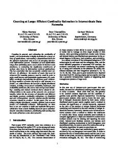
X(k),1
X(k),2
1
1/2
0
Figure 1: An example of the sample (X(k),1 , . . . , X(k),m ), with θ = 7, m = 2, k = 3. The crosses represent the 7 hashed values. This algorithm fulfills the constraints of Problem 1.1, and the memory needed, when expressed in bits, is linear in M := k × m. The distinct elements problem is now reduced to a statistical problem : given a k × m-sample � Ξk,m = X(1),1 , . . . , X(k),1 , . . . , X(1),m , . . . , X(k),m
the distribution of which depends on an unknown parameter θ, one has to find the best estimation of θ. Giroire [5] proposes three different estimators ξ1 , ξ2 , ξ3 , each depending on Ξk,m : ξ1 =
m k−1 X 1 , m X(k),i i=1
ξ2 ξ3
!2 1 p , = C(k, m) X(k),i i=1 ! � � m Γ(k − 1/m) −m 1 X = log X(k),i . exp − Γ(k) m m X
i=1
According to [5], the ξi ’s are asymptotically unbiased: E[ξi ] ∼ θ as θ → +∞. To our knowledge, for the distinct elements problem, Giroire’s algorithms leading to the ξi were the best one-pass algorithms, i.e. producing the estimation with the lowest quadratic error, with ξ3 ahead of the 2 others. One of the goals of this paper is to show that the best (with respect to quadratic error) estimation of θ based on Ξk,m, is given by km − 1 . ξˆ = Pm i=1 X(k),i
1 , the random variables (X(1),i , . . . , X(k−1),i ) are Remark 1.4. Given X(k),i = x < m uniformly distributed on [0, x], i.e. their conditional distribution does not depend on θ. In other words, given X(k),i , the knowledge of the k−1 observations (X(1),i , . . . , X(k−1),i ) ˆ or does not bring any additional information on θ, so it comes as no surprise that ξ, even ξ1 , ξ2 , ξ3 , depend only on X(k),i .
Structure of the paper. The number of values falling in each of the m subintervals follows a multinomial distribution, and, conditionally, given the number of values falling in each of the m subintervals, the distribution of the X(k),i ’s is the distribution of the k-th order statistic of a uniform random sample with random (binomial) size. The
5
PC: y’a un bleme avec la taille des captions
reader surely admits that this description does not sound very tractable. In the next section, we shall thus study the asymptotic distribution of the X(k),i ’s for θ large, for this asymptotic distribution is much simpler than the true distribution. Then we shall prove that ξˆ is the best estimator, provided that the sample Ξk,m follows the asymptotic distribution, and we shall explain the lower bound given by [6]. In the last Section, we discuss the optimality of ξˆ when Ξk,m follows its actual distribution.
2 2.1
The best estimation in the asymptotic model The asymptotic model
First we describe the asymptotic behavior of the X(k),i ’s. Recall that a random variable Γk,θ is said to follow the Gamma distribution with parameters k and θ if P(Γk,θ ∈ [t, t + dt)) =
tk−1 k −θt θ e 1t≥0 dt. Γ(k)
Furthermore, the vector (mθ,i )1≤i≤k of the k smallest among θ i.i.d. random variables, uniform on [0, 1], satisfies (law)
θ (mθ,i )1≤i≤k −−−→ Tk Y, θ→∞
in which the k components of the column vector Y are i.i.d. and follow the exponential distribution with expectation 1, i.e. the Gamma distribution with parameters 1 and 1, and Tk is the k × k matrix with ones on and below the diagonal, and zeroes above the diagonal. As a consequence, (law)
θ mθ,k −−−→ Γk,1 . θ→∞
Since there are approximately θ/m elements in each subinterval, and they are distributed as i.i.d. random variables, uniform on [0, 1/m], we can expect that (law)
(θX(k),1 , . . . , θX(k),m ) −−−→ (Γ(1) , . . . , Γ(m) ), θ→∞
(2)
in which the Γ(i) ’s are m i.i.d. r.v. with common distribution Gamma (k, 1). Also, we can expect θ Ξk,m to be distributed, asymptotically, as m independent copies of Tk Y . Since 1 (law) Γk,1 = Γk,θ , θ equation (2) roughly says that, when θ goes large, the X(k),m behave as m independent random variables with distribution Gamma(k, θ). We shall not prove (2), for we need only a more specific result : the quadratic error is asymptotically the same when the X(k),i ’s are replaced by m independent Gamma random variables. As we shall see later, E[(ξˆ − θ)2 ] = O(θ 2 ). Thus we only need to compare ξˆ to functions f (Ξk,m) such that E[(f (Ξk,m) − θ)2 ] is not too large.
6
Proposition 2.1. Let f be a continuous function: Rm + \{0} → R+ . We assume that outside some neighbourhood of 0, f is bounded, while, in the neighbourhood of 0, there exists r > 0 such that � � 1 |f (x)| = O . (3) k x kr
Then, for any ε > 0, there exists cε > 0 such that, for θ large enough,
h �� �2 � � i E f (X(k),1 , . . . , X(k),m ) − θ 2 − E f (Γ(1) , . . . , Γ(m) ) − θ h i �2 ≤ cε θ ε−1 E f (X(k),1 , . . . , X(k),m ) − θ + 4mθ 2 exp(−θ/(2m)2 ). (4)
in which the Γ(i) ’s are i.i.d. random variables with law Gamma(k, θ).
that θ is large enough, and we shall replace the � Consequently, we shall first assume � X(k),i , i = 1, . . . , m with their limits Γ(i) , i = 1, . . . , m . We know that the X(k),i ’s are large only if θ is small, thus the assumption of boundedness of f outside a neighbourhood of 0 is not really binding for an estimator of θ. Similarly, a good estimation has to be moderately large when the X(k),i ’s are small, thus a good estimation fulfills necessarily (3). The proof of Proposition 2.1 is postponed to Section 2.3.
2.2
Lehmann-Scheff´ e and Cram´ er-Rao inequalities
We are now given a sample (Γ(1) , . . . , Γ(m) ) of m independent Gamma r.v. with parameters (k, θ). We assume that k is known, and we want to estimate the unknown parameter θ. We proceed by maximum likehood estimation: let fθ : Rm + → R+ be the density of the m-sample : fθ (x1 , . . . , xm ) = θ km exp(−θ We are to compute
thus we have to solve :
P
i xi )
Q
xi k−1 i Γ(k) .
� � θˆ := argmaxθ>0 ln fθ (Γ(1) , . . . , Γ(m) ) , 0 = =
� � ∂ ln fθ (Γ(1) , . . . , Γ(m) ) ∂θ X km − Γ(i) , θ i
leading to θ˜ =
Pkm(i) . iΓ
It turns out that this estimator is biased: ˜ =θ E[θ]
km . km − 1
The next Proposition fixes the problem :
7
LG: Terme exponentiellement petit en θ 2 pour ˆ etre tranquille
Proposition 2.2. Set ˆ 1 , . . . , xm ) = ξ(x For any θ,
km − 1 . x1 + · · · + xm
ˆ (1) , . . . , Γ(m) )] = θ, E[ξ(Γ ˆ (1) , . . . , Γ(m) )) = Var(ξ(Γ
θ2 . km − 2
Proof. By stability of the class of Gamma distributions under convolution, γ := Γ(1) + · · · + Γ(m) is Gamma distributed with parameters km and θ. Thus, � � Z +∞ km − 1 (km − 1)θ km E xkm−2 e−θx dx = γ Γ(km) 0 (km − 1)Γ(km − 1) θ = θ. = Γ(km) The variance is obtained through similar computations. Combined with Proposition 2.1, Proposition 2.2 entails that Corollary 2.3. �� �2 � ˆ E ξ(X(k),1 , . . . , X(k),m ) − θ =
θ2 + o(θ 2 ). km − 2
Corollary 2.3 calls for two remarks: 1. the asymptotic variance θ 2 /(km − 2) is indeed smaller than the variance of the estimators proposed in [5], and sets a new record for the lower quadratic error for a one-pass algorithm requiring bounded memory ; 2. since the memory required is linear in km, the quadratic error obtained in Corollary 2.3 is consistent with the theoretical result given in [6]. Let us now recall a few definitions from estimation theory. Given a m-sample (X1 , . . . , Xm ), whose law is denoted Pθ , any random variable S = S(X1 , . . . , Xm ) is (1) (m) called a statistic. P (i)Here, (X1 , . . . , Xm ) = (Γ , . . . , Γ ) and we shall focus on the statistic S = i Γ . First, we check that S fulfills two conditions with deep connections with accuracy : sufficiency and completeness. Definition 2.4. Assume that Pθ admits a density fθ with respect to the Lebesgue measure : 1. a statistic S is said to be sufficient for θ if fθ can be written fθ (x1 , . . . , xm ) = g(S(x1 , . . . , xm ), θ) h(x1 , . . . , xm ), in which g, h are two non-negative measurable functions, h not depending on θ.
8
2. a statistic S is said to be complete if, for any measurable function φ, {∀θ, E[φ(S)] = 0} ⇒ {∀θ, {φ(S) ≡ 0, Pθ − p.s.}} . The next criterion ensures sufficiency and completeness : Proposition 2.5 (see [9],Th.16 Chap.7). Assume that fθ can be written fθ (x) = h(x)B(θ) exp (Q(θ)R(x)) , where h, B, Q, R are measurable functions, h, B being positive. The statistic S(x1 , . . . , xm ) = P R(xi ) is complete and sufficient.
We apply the criterion with h(x) = obtain:
xk−1 Γ(k) ,
Q(θ) = −θ, R(x) = x, B(θ) = 1, we
Corollary 2.6. Under the asymptotic model, S = statistic.
P
iΓ
(i)
is a sufficient and complete
Proposition 2.7 (Lehmann-Scheff´e’s Theorem). [see [9] Th.4, Chap.8] Let S be a complete and sufficient statistic, and let ξ ∗ be an unbiased estimator. The estimator E[ξ ∗ |S] is the unbiased estimator with the lowest variance. It is said to be efficient. Corollary 2.8. Let ξ˜ be an unbiased estimator of θ. E[(ξ˜ − θ)2 ] ≥ E[(ξˆ − θ)2 ] =
θ2 . km − 2
(5)
P (i) and ξ ∗ = ξ, ˆ This is a consequence of Lehmann-Scheff´e’s Theorem with S = m i=1 Γ ˆ = ξ. ˆ This inequality is sharp for our model, but it is valid only for unbiased since E[ξ|S] estimators. Cram´er-Rao inequality [8, Th. 6.4, page 122] gives a more general lower bound :
Proposition 2.9 (Cram´er-Rao inequality). Let gθ be the density of Γ(1) . Assume that θ 7→ log gθ (x) is continuously differentiable, and that the quantity � 2 � d (1) I(θ) = −E log gθ (Γ ) dθ 2 is finite and positive. Let ξ ∗ be a square-integrable function such that b(θ) := E[ξ ∗ ] − θ is continuously differentiable. then � � (1 + b′ (θ))2 + b(θ)2 . E (ξ ∗ − θ)2 ≥ mI(θ)
In particular, if ξ ∗ is unbiased, its variance is bounded from below by 1/mI(θ).
9
The quantity I(θ) is the Fisher information. In our case, it reduces to " !# d2 (Γ(1) )k−1 θ k −θΓ(1) I(θ) = −E , log e dθ 2 Γ(k) � 2 � �� d (1) k log θ − θΓ , = −E dθ 2 k = 2. θ Under the asymptotic model, Cram´er-Rao inequality reads E[(ξ ∗ − θ)2 ] ≥ (1 + b′ (θ))2
θ2 + b(θ)2 , km
(6)
for any estimator ξ ∗ such that θ 7→ E[ξ ∗ ] is continuously differentiable. Cram´er-Rao inequality confirms that quadratic error cannot decrease faster than θ 2 /M . The estimator ξˆ achieves this lower bound, up to a factor km/(km − 2).
2.3
Proof of Proposition 2.1
Let A be the event A = Ak,m,θ ={For any 1 ≤ i ≤ m, at least k hashed values lie in the i-th interval} ={For any 1 ≤ i ≤ m, X(k),i
0, � h �2 i� , I = O θ ε−1 E f (X(k),1 , . . . , X(k),m ) − θ in which I is defined below :
I = I1 − I2 , P Z m θ−mk Y xi k−1 2 θ! (1 − i xi ) (f (x) − θ) I1 = dx, (θ − km)! Γ(k) [0,1/m]m i=1 Z m Y X xi k−1 dx. (f (x) − θ)2 θ km exp(−θ xi ) I2 = Γ(k) Rm + i=1
i
P By the substitution yi = θxi , and with the notation s = i yi , we get Z θ−mk Y y k−1 i (f (y/θ) − θ)2 θ!(1−(s/θ)) I1 = dy, (θ−km)!θ km Γ(k) m [0,θ/m] i≤m Z m Y yi k−1 2 dy. (f (y/θ) − θ) exp(−s) I2 = Γ(k) Rm +
(9) (10)
i=1
Set F (y, θ) = 1 −
(θ − km)! θ km exp(−s) . �θ−mk θ! 1 − θs
We write I = J − K, with Z F (y, θ) (f (y/θ) − θ)2 J= [0,θ/m]m
K=
Z
m Rm + \[0,θ/m]
θ!(1−(s/θ))θ−mk (θ−km)!θ km
Y yi k−1 dy, Γ(k)
i≤m
(f (y/θ) − θ)2 exp(−s)
m Y i=1
k−1
yi dy. Γ(k)
We will show that these two integrals are o(θ 2 ). Since f is continuous and bounded away� from� zero outside some neighbourhood of 0, there exist c, c′ > 0 such that in θ m Rm , when θ is large enough, + \ 0, m |f (y/θ) − θ|2 ≤ c + θ 2 ≤ c′ θ 2 .
Then ′ 2
|K| ≤ c θ
Z
m
θ Rm + \[0, m ]
11
Y yi k−1 e−s dy Γ(k)
i≤m
that vanishes exponentially fast, the integral on the right hand side being the probability that the maximum of an m-sample of Gamma distributed random variables is larger than θ/m. Let us write J = J1 + J2 in which Z θ−mk Y y k−1 i F (y, θ) (f (y/θ) − θ)2 θ!(1−(s/θ)) J1 = dy, (θ−km)!θ km Γ(k) α m [0,θ /m] i≤m Z Y yi k−1 2 θ!(1−(s/θ))θ−mk dy. F (y, θ) (f (y/θ) − θ) J2 = km (θ−km)!θ m α m Γ(k) [0, θ ] \[0, θ ] m
i≤m
m
and assume that α ∈ (0, 1/2). Let F (y, θ) = 1 − eψ(s,θ) , in which ψ(s, θ) = −s − θ ln 1 − =O θ
2α−1
�
s θ
�
+O θ
+ mk ln 1 − α−1
�
+O θ
s θ
−1
�
�
,
−
km−1 X ℓ=1
ln 1 −
ℓ θ
�
as long as y ∈ [0, θ α /m]m . Using (9), we conclude that there exists cα > 0 such that for, θ large enough, h �2 i J1 ≤ cα θ 2α−1 I1 ≤ cα θ 2α−1 E f (X(k),1 , . . . , X(k),m ) − θ . As concerns J2 , we write J2 = J2,1 − J2,2 , with Z Y yi k−1 2 −s (f (y/θ) − θ) e dy, J2,1 = m Γ(k) [0, mθ ] \[0,θα /m]m i≤m Z Y yi k−1 2 θ!(1−(s/θ))θ−mk dy. (f (y/θ) − θ) J2,2 = (θ−km)!θ km m Γ(k) [0, mθ ] \[0,θα /m]m i≤m
First, we bound J2,1 : �by the second assumption of Proposition 2.1, there exist c, c′ > 0 � � � α m m θ \ 0, θm , such that, for all y ∈ 0, m
|f (y/θ) − θ|2 ≤ θ 2 + f 2 (y/θ) 1 ≤ θ2 + c 1∧ k y/θ k2r c′ θ 2r ≤ , k y k2r � θ �m � θ α �m in which r can be chosen larger than 1. Since y ∈ 0, m \ 0, m , we have s ≥ θ α /m. It follows that Z c′ θ 2r e−s Y yi k−1 J2,1 ≤ dy. 2r m Γ(k) [0, mθ ] \[0,θα /m]m k y k i≤m Z Y yi k−1 dy α , ≤ c′ θ 2r e−θ /m m θ m Γ(k) k y k2r α [0, m ] \[0,θ /m] i≤m
12
in which the last integral is polynomial in θ. For J2,2 , we have, as soon as θ ≥ 2mk, θ!(1−(s/θ))θ−mk (θ−km)!θ km
≤ (1 − (s/θ))θ/2 ≤ exp(−s/2).
Thus, by the same argument, J2,2 vanishes exponentially fast. To finish the proof, take ε = 2α.
3
Optimality of ξˆ
We return to the original model, in which X(k),i denotes the k-th smallest value lying i in [ i−1 m , m ). We wish to discuss the optimality of km − 1 ξˆ = Pm . i=1 X(k),i
The combination of (5) and (6) gives the following result, which is the main result of the present work. ˆ Let ξ˜ = ξ(x) ˜ Theorem 3.1 (Optimality of ξ). be a continuous function on Rm + − {0}. Assume that there exists r > 0 such that, in the neighbourhood of 0, � � 1 . |f (x)| = O k x kr The application
˜ (1) , . . . , Γ(m) )] − θ, b(θ) := E[ξ(Γ
is continuously differentiable, and ˜ (k),1 , . . . , X(k),m ) − θ)2 ] ≥ E[(ξ(X
�2 θ2 1 + b′ (θ) + o(θ 2 ). km
If we assume furthermore that ξ˜ is unbiased in the asymptotic model i.e. ˜ 1 , . . . , Γm )] = θ, E[ξ(Γ
(11)
then ˜ (k),1 , . . . , X(k),m ) − θ)2 ] ≥ E[(ξˆ − θ)2 ] + o(θ 2 ), E[(ξ(X =
θ2 + o(θ 2 ). km − 2
Remark 3.2. The second assumption (ξ˜ unbiased in the asymptotic model) was implicitly made in [5]. Proof. Proposition 2.1 with ε = 1/2 implies that there exists c > 0 such that, for θ large enough, ˜ (k),1 , . . . , X(k),m ) − θ)2 ] ≥ E[ξ(Γ ˜ 1 , . . . , Γm )] − cθ −1/2 E[(ξ(X ˜ (k),1 , . . . , X(k),m ) − θ)2 ] + o(θ 2 ), E[(ξ(X �2 θ2 ˜ (k),1 , . . . , X(k),m ) − θ)2 ] + o(θ 2 ) 1 + b′ (θ) − cθ −1/2 E[(ξ(X ≥ km
13
by (6). The conclusion of the Theorem follows : if E[(ξ˜ − θ)2 ] is larger than, say, θ 7/3 then there is nothing to prove ; if it is smaller then the right-hand term is
LG: Petite modif de la preuve pour ˆ etre plus clair
�2 θ2 1 + b′ (θ) + o(θ 2 ). km
If we assume furthermore that (11) holds, then (5) gives the second assertion of the theorem.
3.1
The case m = 1
The lower bound given by Theorem 3.1 depends on the choice of (k, m) only through the product km. Thus, regardless of algorithmic considerations, the quadratic error does not benefit from the partition of [0, 1] in m sub-intervals, and we may assume m = 1 to study the optimality of our estimator. When m = 1, the law of the observation X(k),1 is easy to deal with, and we obtain a sharp and exact lower bound (i.e. valid for any θ). The irrelevance, with respect to statistics, of splitting [0, 1] into m subintervals, is perhaps clearer in the asymptotic model. We noted in Section 2.1 that Ξk,m is distributed, asymptotically, as m independent copies of Tk Y , in which Y is a k-sample of the exponential distribution with expectation 1/θ, and Tk Y = (Y1 , Y1 + Y2 , Y1 + Y2 + Y3 , . . . , Y1 + Y2 + · · · + Yk ). From a statistical perspective, since Tk is one-to-one, there is no loss of information from Y to Tk Y . Thus, for the estimation of θ, Ξk,m is equivalent to m independent copies of a k-sample of the exponential distribution with expectation 1/θ, i.e. a km-sample of the exponential distribution with expectation 1/θ. But this is also equivalent to Tkm Yˆ , in which Yˆ is a km-sample of the exponential distribution with expectation 1/θ : we can obtain Tkm Yˆ as the asymptotic distribution of the first km order statistics of a θ-sample of uniform random variables on [0, 1], that is, without splitting the interval [0, 1] into m subintervals. For the exponential distribution, the sum of the km elements of the sample is known to be complete and sufficient : when splitting, this corresponds to the sum of the m copies of the k-th order statistic, and when not splitting, this sum is asymptotic to the km-th order statistic. Theorem 3.3. Consider algorithm MinCount, with parameter m = 1. It returns ˆ (k) ) = k − 1 . ξ(X X(k) For any θ, ξˆ is an unbiased estimator. Furthermore, ξˆ is the unbiased estimator with the lowest variance. Note that in this particular case m = 1, our estimator coincides with the estimator ξ1 proposed by Giroire.
14
LG: Petite remarque ajout´ ee
Proof. We know from (1) that ξˆ is unbiased. We apply the Lehmann-Scheff´e Theorem to the law Qθ of X(k) . �
� θ − 1 k−1 Qθ (x)dx = θ x (1 − x)θ−k dx k−1 = B(θ)h(x) exp((θ − k) log(1 − x))dx, with notations of Proposition 2.5. This shows that the statistic log(1−X(k) ) is complete and sufficient. Thus the variance of the statistic � � k − 1 k−1 E log(1 − X(k) ) = X(k) X(k)
is minimal.
References [1] N. Alon, Y. Matias, and M. Szegedy. The space complexity of approximating the frequency moments. Journal of Computer and System Sciences, 58:137–147, 1999. [2] Ph. Chassaing and L. Gerin. Efficient estimation of the cardinality of large data sets. In DMTCS Proceedings of Fourth Colloquium on Mathematics and Computer Science, pages 419–422, 2006. [3] H.A. David. Order statistics. Wiley & Sons, 1981. [4] Ph. Flajolet and N. Martin. Probabilistic counting algorithms for data base applications. Journal of Computer and System Sciences, 31:182–209, 1985. [5] F. Giroire. Order statistics and estimating cardinalities of massive data sets. Discrete Applied Mathematics, 157:406–427, 2009. [6] P. Indyk and D. Woodruff. Tight lower bounds for the distinct elements problem. In Proceedings of the 44th IEEE Symposium on Foundations of Computer Science, Boston, 2003. [7] D.E. Knuth. The Art of Computer Programming, vol. 3 : Sorting and Searching. Addison-Wesley, 1973. [8] E.L. Lehmann. Theory of Point Estimation. John Wiley & sons, 1983. [9] B.W. Lindgren. Statistical Theory. Chapman & Hall, 4th edition, 1993. [10] R. Morris. Counting large numbers of events in small registers. Communications of the ACM, 21:840–842, 1978. [11] V. Vapnik. The nature of statistical learning theory. Springer, 1995.
15


![[math.ST] 22 Apr 2011 Efficient estimation of the cardinality of large ...](https://m.moam.info/img/260x300/mathst-22-apr-2011-efficient-estimation-of-the-car_59d3905f1723dd016121010b.jpg)
![arXiv:1104.4481v1 [hep-ex] 22 Apr 2011](https://m.moam.info/img/260x300/arxiv11044481v1-hep-ex-22-apr-2011_5ba0de93097c47f3698b4593.jpg)
![arXiv:1605.00591v3 [q-bio.QM] 22 Apr 2018](https://m.moam.info/img/260x300/arxiv160500591v3-q-bioqm-22-apr-2018_5b78c35f097c47be638b46c4.jpg)
![arXiv:1804.08114v1 [math.KT] 22 Apr 2018 - UOW](https://m.moam.info/img/260x300/arxiv180408114v1-mathkt-22-apr-2018-uow_5b78c400097c47a90e8b456b.jpg)
![arXiv:1504.05945v1 [gr-qc] 22 Apr 2015](https://m.moam.info/img/260x300/arxiv150405945v1-gr-qc-22-apr-2015_5b7b2ee4097c47b7098b4573.jpg)
![arXiv:1504.05834v1 [math.PR] 22 Apr 2015](https://m.moam.info/img/260x300/arxiv150405834v1-mathpr-22-apr-2015_5c1aaa11097c47bf738b4608.jpg)
![arXiv:1603.02251v3 [hep-th] 22 Apr 2016](https://m.moam.info/img/260x300/arxiv160302251v3-hep-th-22-apr-2016_5add1b967f8b9a861e8b4613.jpg)
![arXiv:0904.3409v1 [astro-ph.HE] 22 Apr 2009](https://m.moam.info/img/260x300/arxiv09043409v1-astro-phhe-22-apr-2009_5c1caea3097c475e158b456b.jpg)
![arXiv:1803.05509v2 [quant-ph] 22 Apr 2018](https://m.moam.info/img/260x300/arxiv180305509v2-quant-ph-22-apr-2018_5ba3b3a1097c47731a8b46f5.jpg)
![arXiv:1804.08064v1 [cs.CL] 22 Apr 2018 - Wisc](https://m.moam.info/img/260x300/arxiv180408064v1-cscl-22-apr-2018-wisc_5c934eaa097c47862f8b4621.jpg)
![arXiv:1504.05655v1 [cs.SI] 22 Apr 2015](https://m.moam.info/img/260x300/arxiv150405655v1-cssi-22-apr-2015_5ca0bb0e097c47dc4e8b4679.jpg)
![arXiv:1703.04701v2 [math.DG] 22 Apr 2017](https://m.moam.info/img/260x300/arxiv170304701v2-mathdg-22-apr-2017_5b78c360097c47bf638b46da.jpg)
![arXiv:1701.04773v2 [gr-qc] 22 Apr 2017](https://m.moam.info/img/260x300/arxiv170104773v2-gr-qc-22-apr-2017_5b78c371097c47bd638b46d6.jpg)
![arXiv:1804.08084v1 [math.AP] 22 Apr 2018](https://m.moam.info/img/260x300/arxiv180408084v1-mathap-22-apr-2018_5b78c3df097c47bd638b46ec.jpg)
![arXiv:1004.3962v1 [hep-th] 22 Apr 2010](https://m.moam.info/img/260x300/arxiv10043962v1-hep-th-22-apr-2010_5c608991097c4795408b45db.jpg)
![arXiv:1709.08420v2 [physics.soc-ph] 22 Apr 2018](https://m.moam.info/img/260x300/arxiv170908420v2-physicssoc-ph-22-apr-2018_5bb012df097c47d7188b4786.jpg)
![arXiv:1103.5786v2 [astro-ph.CO] 10 Apr 2011](https://m.moam.info/img/260x300/arxiv11035786v2-astro-phco-10-apr-2011_5c933dd9097c4797138b45ff.jpg)
![arXiv:1104.2501v1 [astro-ph.HE] 13 Apr 2011](https://m.moam.info/img/260x300/arxiv11042501v1-astro-phhe-13-apr-2011_5c1f4624097c47b97b8b45d8.jpg)
![arXiv:1104.3883v1 [quant-ph] 19 Apr 2011](https://m.moam.info/img/260x300/arxiv11043883v1-quant-ph-19-apr-2011_647a1e97097c476c028c5ad2.jpg)
![arXiv:1103.5433v5 [cs.NI] 25 Apr 2011](https://m.moam.info/img/260x300/arxiv11035433v5-csni-25-apr-2011_59a6074b1723dd0c40321663.jpg)
![arXiv:1104.4298v1 [cs.CV] 21 Apr 2011 - CiteSeerX](https://m.moam.info/img/260x300/arxiv11044298v1-cscv-21-apr-2011-citeseerx_5a9c9a1a1723dd23c077ecc2.jpg)
![arXiv:1104.5052v1 [math.HO] 27 Apr 2011](https://m.moam.info/img/260x300/arxiv11045052v1-mathho-27-apr-2011_5b9b3b46097c4792718b4663.jpg)
![arXiv:1104.4175v1 [math.CV] 21 Apr 2011](https://m.moam.info/img/260x300/arxiv11044175v1-mathcv-21-apr-2011_5c2d7ac7097c4784048b45ae.jpg)