University College of Southeast Norway
MATLAB Part II: Modelling, Simulation & Control Hans-Petter Halvorsen, 2016.06.22
http://home.hit.no/~hansha
Table of Contents 1
Introduction ...................................................................................................................... 4
2
Differential Equations and ODE Solvers ............................................................................ 5 Task 1: Bacteria Population ....................................................................................... 5 Task 2: Passing Parameters to the model .................................................................. 6 Task 3: ODE Solvers ................................................................................................... 7 Task 4: 2.order differential equation ......................................................................... 9
3
Discrete Systems ............................................................................................................. 12 Task 5: Discrete Simulation ..................................................................................... 12 Task 6: Discrete Simulation – Bacteria Population .................................................. 14 Task 7: Simulation with 2 variables ......................................................................... 15
4
Numerical Techniques ..................................................................................................... 18 Task 8: Interpolation ................................................................................................ 18 Task 9: Linear Regression ........................................................................................ 20
5
Task 10:
Polynomial Regression ............................................................................. 21
Task 11:
Model fitting ............................................................................................ 22
Task 12:
Numerical Differentiation ........................................................................ 25
Task 13:
Differentiation on Polynomials ................................................................ 28
Task 14:
Differentiation on Polynomials ................................................................ 29
Task 15:
Numerical Integration ............................................................................. 30
Task 16:
Integration on Polynomials ..................................................................... 32
Optimization .................................................................................................................... 34 Task 17:
Optimization ............................................................................................ 34
Task 18:
Optimization - Rosenbrock's Banana Function ........................................ 35 MATLAB Course, Part II - Solutions
6
Control System Toolbox .................................................................................................. 38
7
Transfer Functions ........................................................................................................... 39
8
9
10
Task 19:
Transfer function ..................................................................................... 39
Task 20:
2. order Transfer function ....................................................................... 40
Task 21:
Time Response ........................................................................................ 43
Task 22:
Integrator ................................................................................................ 44
Task 23:
1. order system ........................................................................................ 48
Task 24:
2. order system ........................................................................................ 53
Task 25:
2. order system – Special Case ................................................................ 56
State-Space Models ......................................................................................................... 59 Task 26:
State-space model ................................................................................... 59
Task 27:
Mass-spring-damper system ................................................................... 61
Task 28:
Block Diagram .......................................................................................... 63
Task 29:
Discretization ........................................................................................... 64
Frequency Response ....................................................................................................... 66 Task 30:
1. order system ........................................................................................ 66
Task 31:
Bode Diagram .......................................................................................... 71
Task 32:
Frequency Response Analysis .................................................................. 73
Task 33:
Stability Analysis ...................................................................................... 78
Additional Tasks .......................................................................................................... 82 Task 34:
ODE Solvers ............................................................................................. 82
Task 35:
Mass-spring-damper system ................................................................... 83
Task 36:
Numerical Integration ............................................................................. 85
Task 37:
State-space model ................................................................................... 87
Task 38:
lsim .......................................................................................................... 89
MATLAB Course, Part II - Solutions
1 Introduction No Tasks
4
2 Differential Equations and ODE Solvers Task 1:
Bacteria Population
In this task we will simulate a simple model of a bacteria population in a jar. The model is as follows:
birth rate=bx death rate = px2 Then the total rate of change of bacteria population is: 𝑥 = 𝑏𝑥 − 𝑝𝑥 2 Set b=1/hour and p=0.5 bacteria-hour → Simulate the number of bacteria in the jar after 1 hour, assuming that initially there are 100 bacteria present. [End of Task]
Solution: We define the function for the differential equation: function dx = bacteriadiff(t,x) % My Simple Differential Equation b=1; p=0.5; dx = b*x - p*x^2; We create a script to solve the differential equation using a ode function: tspan=[0 1]; x0=100; 5
6
Differential Equations and ODE Solvers
[t,y]=ode45(@bacteriadiff, tspan,x0); plot(t,y) The result becomes:
Task 2:
Passing Parameters to the model
Given the following system: 𝑥 = 𝑎𝑥 + 𝑏 5
where 𝑎 = − ,where 𝑇 is the time constant 6
In this case we want to pass a and b as parameters, to make it easy to be able to change values for these parameters We set initial condition 𝑥(0) = 1 and 𝑇 = 5. The function for the differential equation is: function dx = mysimplediff(t,x,param) % My Simple Differential Equation a=param(1); b=param(2);
MATLAB Course, Part II - Solutions
7
Differential Equations and ODE Solvers
dx=a*x+b; Then we solve and plot the equation using this code: tspan=[0 25]; x0=1; a=-1/5; b=1; param=[a b]; [t,y]=ode45(@mysimplediff, tspan, x0,[], param); plot(t,y) By doing this, it is very easy to changes values for the parameters a and b. Note! We need to use the 5. argument in the ODE solver function for this. The 4. argument is for special options and is normally set to “[]”, i.e., no options. The result from the simulation is:
→ Write the code above Read more about the different solvers that exists in the Help system in MATLAB [End of Task]
Task 3:
ODE Solvers MATLAB Course, Part II - Solutions
8
Differential Equations and ODE Solvers
Use the ode23 function to solve and plot the results of the following differential equation in the interval [𝑡? , 𝑡A ]: 𝒘D + 𝟏. 𝟐 + 𝒔𝒊𝒏𝟏𝟎𝒕 𝒘 = 𝟎, 𝑡? = 0, 𝑡A = 5, 𝑤 𝑡? = 1 [End of Task]
Solution: We start by rewriting the differential equation: 𝑤 D = − 1.2 + 𝑠𝑖𝑛10𝑡 𝑤 This gives: function dw = diff_task3(t,w) dw = -(1.2 + sin(10*t))*w; The Script for solving the equation: tspan=[0 5]; w0=1; [t,w]=ode23(@diff_task3, tspan, w0); plot(t,w) This gives:
MATLAB Course, Part II - Solutions
9
Task 4:
Differential Equations and ODE Solvers
2.order differential equation
Use the ode23/ode45 function to solve and plot the results of the following differential equation in the interval [𝑡? , 𝑡A ]: 𝟏 + 𝒕𝟐 𝒘 + 𝟐𝒕𝒘 + 𝟑𝒘 = 𝟐, 𝑡? = 0, 𝑡A = 5, 𝑤 𝑡? = 0, 𝑤 𝑡? = 1 Note! Higher order differential equations must be reformulated into a system of first order differential equations. Tip 1: Reformulate the differential equation so 𝑤 is alone on the left side. Tip 2: Set: 𝑤 = 𝑥5 𝑤 = 𝑥2 [End of Task]
Solution: First we rewrite like this: 𝑤=
2 − 2𝑡𝑤 − 3𝑤 1 + 𝑡2
In order to solve it using the ode functions in MATLAB it has to be a set with 1.order ode’s. So we set: 𝑤 = 𝑥5 𝑤 = 𝑥2 This gives: 𝑥5 = 𝑥2 𝑥2 =
2 − 2𝑡𝑥2 − 3𝑥5 1 + 𝑡2
Now we can use MATLAB to solve the equations: function dx = diff_secondorder(t,x) [m,n] = size(x); dx = zeros(m,n)
MATLAB Course, Part II - Solutions
10
Differential Equations and ODE Solvers
dx(1) = x(2); dx(2) = (2-2*t*x(2)-3*x(1))/(1+t^2); and: tspan=[0 5]; x0=[0; 1]; [t,x]=ode23(@diff_secondorder, tspan, x0); plot(t,x) legend('x1','x2') This gives:
if we want to plot only 𝑤 = 𝑥5 we can use plot(t,x(:,1)) Like this: tspan=[0 5]; x0=[0; 1]; [t,x]=ode23(@diff_secondorder, tspan, x0); plot(t, x(:,2)) This gives:
MATLAB Course, Part II - Solutions
11
Differential Equations and ODE Solvers
So the solution to: 𝟏 + 𝒕𝟐 𝒘 + 𝟐𝒕𝒘 + 𝟑𝒘 = 𝟐, 𝑡? = 0, 𝑡A = 5, 𝑤 𝑡? = 0, 𝑤 𝑡? = 1 is the plot above.
MATLAB Course, Part II - Solutions
3 Discrete Systems Task 5:
Discrete Simulation
Given the following differential equation: 𝑥 = 𝑎𝑥 5
where 𝑎 = − , where 𝑇 is the time constant 6
Note! 𝑥 =
ST SU
Find the discrete differential equation and plot the solution for this system using MATLAB. Set 𝑇 = 5 and the initial condition 𝑥(0) = 1. Create a script in MATLAB (.m file) where we plot the solution 𝑥(𝑘). [End of Task]
Solution: We can use e.g., the Euler Approximation: 𝑥≈
𝑥XY5 − 𝑥X 𝑇Z
Then we get: 𝑥XY5 − 𝑥X = 𝑎𝑥X 𝑇Z Which gives: 𝑥XY5 = 𝑥X (1 + 𝑇Z 𝑎) MATLAB Code: % Simulation of discrete model clear, clc % Model Parameters T = 5; 12
13
Discrete Systems
a = -1/T; % Simulation Parameters Ts = 0.1; %s Tstop = 30; %s x(1) = 1; % Simulation for k=1:(Tstop/Ts) x(k+1) = (1+a*Ts).*x(k); end % Plot the Simulation Results k=0:Ts:Tstop; plot(k,x) grid on Plot:
MATLAB Course, Part II - Solutions
14
Task 6:
Discrete Systems
Discrete Simulation – Bacteria Population
In this task we will simulate a simple model of a bacteria population in a jar. The model is as follows:
birth rate=bx death rate = px2 Then the total rate of change of bacteria population is: 𝑥 = 𝑏𝑥 − 𝑝𝑥 2 Set b=1/hour and p=0.5 bacteria-hour We will simulate the number of bacteria in the jar after 1 hour, assuming that initially there are 100 bacteria present. → Find the discrete model using the Euler Forward method by hand and implement and simulate the system in MATLAB using a For Loop. [End of Task]
Solution: We create a discrete model. and use Euler Forward differentiation method: 𝑥≈
𝑥XY5 − 𝑥X 𝑇Z
Where 𝑇Z is the Sampling Time. We get: 𝑥XY5 − 𝑥X = 𝑏𝑥X − 𝑝𝑥X2 𝑇Z This gives: 𝑥XY5 = 𝑥X + 𝑇Z (𝑏𝑥X − 𝑝𝑥X2 ) We implement the model in MATLAB: clc % Model Parameters b = 1; MATLAB Course, Part II - Solutions
15
Discrete Systems
p = 0.5; % Simulation Parameters Ts=0.01; x(1)=100; k=1; % Simulation Loop for i=Ts:Ts:1 % Discrete model x(k+1) = x(k) + Ts*(b.*x(k) - p*x(k).^2); k=k+1; end % Plot the simulation results i = 0:Ts:1; plot(x, i) The simulation result becomes:
Task 7:
Simulation with 2 variables
Given the following system 𝑑𝑥5 = −𝑥2 𝑑𝑡 𝑑𝑥2 = 𝑥5 𝑑𝑡 MATLAB Course, Part II - Solutions
16
Discrete Systems
Find the discrete system and simulate the discrete system in MATLAB. [End of Task]
Solution: Using Euler gives: 𝑥5 𝑘 + 1 = 𝑥5 𝑘 − 𝑇Z 𝑥2 𝑘 𝑥2 𝑘 + 1 = 𝑥2 𝑘 + 𝑇Z 𝑥5 𝑘 MATLAB Code: % Simulation of discrete model clear, clc % Model Parameters T = 5; a = -1/T; % Simulation Parameters Ts = 0.1; %s Tstop = 10; %s x1(1) = 1; x2(1) = 1; % Simulation for k=1:(Tstop/Ts) x1(k+1) = x1(k) - Ts.*x2(k); x2(k+1) = x2(k) + Ts.*x1(k); end % Plot the Simulation Results k=0:Ts:Tstop; plot(k,x1,k,x2) grid on Plot:
MATLAB Course, Part II - Solutions
17
Discrete Systems
MATLAB Course, Part II - Solutions
4 Numerical Techniques Task 8:
Interpolation
Given the following data: Temperature, T [ oC] 100 150 200 250 300 400 500
Energy, u [KJ/kg] 2506.7 2582.8 2658.1 2733.7 2810.4 2967.9 3131.6
Plot u versus T. Find the interpolated data and plot it in the same graph. Test out different interpolation types. What is the interpolated value for u=2680.78 KJ/kg? [End of Task]
Solution: MATLAB Script: T = [100, 150, 200, 250, 300, 400, 500]; u=[2506.7, 2582.8, 2658.1, 2733.7, 2810.4, 2967.9, 3131.6]; figure(1) plot(u,T, '-o') % Find interpolated value for u=2680.78 new_u=2680.78; interp1(u, T, new_u) %Spline new_u = linspace(2500,3200,length(u)); new_T = interp1(u, T, new_u, 'spline'); figure(2) plot(u,T, new_u, new_T, '-o') 18
19
Numerical Techniques
The interpolated value for u=2680.78 KJ/kg is: ans = 215.0000 i., for 𝑢 = 2680.76 we get 𝑇 = 215. The plot becomes:
For spline, cubic we get almost the same:
This is because the points listed above are quite linear in their nature. MATLAB Course, Part II - Solutions
20
Task 9:
Numerical Techniques
Linear Regression
Given the following data: Temperature, T [ oC] 100 150 200 250 300 400 500
Energy, u [KJ/kg] 2506.7 2582.8 2658.1 2733.7 2810.4 2967.9 3131.6
Plot u versus T. Find the linear regression model from the data 𝑦 = 𝑎𝑥 + 𝑏 Plot it in the same graph. [End of Task]
Solution: MATLAB Script: T = [100, 150, 200, 250, 300, 400, 500]; u=[2506.7, 2582.8, 2658.1, 2733.7, 2810.4, 2967.9, 3131.6]; n=1; % 1.order polynomial(linear regression) p=polyfit(u,T,n); a=p(1) b=p(2), x=u; ymodel=a*x+b; plot(u,T,'o',u,ymodel) a = 0.6415 b = -1.5057e+003 MATLAB Course, Part II - Solutions
21
Numerical Techniques
i., we get a polynomial 𝑝 = [0.6, −1.5 ∙ 10b ]. The Plot becomes:
Task 10:
Polynomial Regression
Given the following data: x 10 20 30 40 50 60 70 80 90 100
y 23 45 60 82 111 140 167 198 200 220
→ Use the polyfit and polyval functions in MATLAB and compare the models using different orders of the polynomial. Use subplots and make sure to add titles, etc.
MATLAB Course, Part II - Solutions
22
Numerical Techniques [End of Task]
Solution: MATLAB Script: x=[10, 20, 30, 40, 50, 60, 70, 80, 90, 100]; y=[23, 45, 60, 82, 111, 140, 167, 198, 200, 220]; for n=2:5 p=polyfit(x,y,n); ymodel=polyval(p,x)
end
subplot(2,2,n-1) plot(x,y,'o',x,ymodel) title(sprintf('Model of order %d', n));
The result is:
Task 11:
Model fitting
Given the following data: MATLAB Course, Part II - Solutions
23
Height, h[ft] 0 1.7 1.95 2.60 2.92 4.04 5.24
Numerical Techniques
Flow, f[ft^3/s] 0 2.6 3.6 4.03 6.45 11.22 30.61
→ Create a 1. (linear), 2. (quadratic) and 3.order (cubic) model. Which gives the best model? Plot the result in the same plot and compare them. Add xlabel, ylabel, title and a legend to the plot and use different line styles so the user can easily see the difference. [End of Task]
Solution: MATLAB Script: clear, % Real height flow =
clc Data = [0, 1.7, 1.95, 2.60, 2.92, 4.04, 5.24]; [0, 2.6, 3.6, 4.03, 6.45, 11.22, 30.61];
new_height = 0:0.5:6; % generating new height values used to test the model %linear------------------------polyorder = 1; %linear p1 = polyfit(height, flow, polyorder) % 1.order model new_flow1 = polyval(p1,new_height); % We use the model to find new flow values %quadratic------------------------polyorder = 2; %quadratic p2 = polyfit(height, flow, polyorder) % 2.order model new_flow2 = polyval(p2,new_height); % We use the model to find new flow values %cubic------------------------polyorder = 3; %cubic p3 = polyfit(height, flow, polyorder) % 3.order model new_flow3 = polyval(p3,new_height); % We use the model to find new flow values %Plotting %We plot the original data together with the model found for comparison MATLAB Course, Part II - Solutions
24
Numerical Techniques
plot(height, flow, 'o', new_height, new_flow1, new_height, new_flow2, new_height, new_flow3) title('Model fitting') xlabel('height') ylabel('flow') legend('real data', 'linear model', 'quadratic model', 'cubic model') The result becomes: p1 = 5.3862 p2 = 1.4982 p3 = 0.5378
-5.8380 -2.5990
1.1350
-2.6501
4.9412
-0.1001
Where p1 is the linear model (1.order), p2 is the quadratic model (2.order) and p3 is the cubic model (3.order). This gives: 1. order model: 𝑝5 = 𝑎? 𝑥 + 𝑎5 = 5.4𝑥 − 5.8 2. order model: 𝑝2 = 𝑎? 𝑥 2 + 𝑎5 𝑥 + 𝑎2 = 1.5𝑥 2 − 2.6𝑥 + 1.1 3. order model: 𝑝b = 𝑎? 𝑥 b + 𝑎5 𝑥 2 + 𝑎2 𝑥 + 𝑎b = 0.5𝑥 b − 2.7𝑥 2 + 4.9𝑥 − 0.1 We get the following plot:
MATLAB Course, Part II - Solutions
25
Numerical Techniques
Discussion: As you see the cubic model (3.order) gives the best result, i.e., the cubic model fits the data best.
Task 12:
Numerical Differentiation
Given the following equation: 𝑦 = 𝑥 b + 2𝑥 2 − 𝑥 + 3 Find
Se ST
analytically (use “pen and paper”).
Define a vector x from -5 to +5 and use the diff function to approximate the derivative y with ∆e
respect to x ( ). ∆T
Compare the data in a 2D array and/or plot both the exact value of approximation in the same plot. Increase number of data point to see if there are any difference.
MATLAB Course, Part II - Solutions
Se ST
and the
26
Numerical Techniques
Do the same for the following functions: 𝑦 = sin (𝑥) 𝑦 = 𝑥 i − 1 [End of Task]
Solution: Analytically solution: 𝑑𝑦 = 3𝑥 2 + 4𝑥 − 1 𝑑𝑥 MATLAB Script: x = -5:1:5; % Define the function y(x) y = x.^3 + 2*x.^2 - x + 3; % Plot the function y(x) plot(x,y) title('y') % Find nummerical solution to dy/dx dydx_num = diff(y)./diff(x); dydx_exact = 3*x.^2 + 4.*x -1; dydx = [[dydx_num, NaN]', dydx_exact'] % Plot nummerical vs analytical solution to dy/dx figure(2) plot(x,[dydx_num, NaN], x, dydx_exact) title('dy/dx') legend('numerical solution', 'analytical solution') Plot of 𝑦(𝑥):
MATLAB Course, Part II - Solutions
27
Numerical Techniques
Plot of
Se ST
(Analytical vs. numerical solution):
The values are: dydx = 42 22
54 31 MATLAB Course, Part II - Solutions
28
8 0 -2 2 12 28 50 78 NaN
Numerical Techniques
14 3 -2 -1 6 19 38 63 94
We do the same for the following functions: 𝑦 = sin (𝑥) 𝑑𝑦 = cos (𝑥) 𝑑𝑥 𝑦 = 𝑥 i − 1 𝑑𝑦 = 5𝑥 l 𝑑𝑥 → The procedure is exactly the same and will not be shown here.
Task 13:
Differentiation on Polynomials
Consider the following equation: 𝑦 = 𝑥 b + 2𝑥 2 − 𝑥 + 3 Use Differentiation on the Polynomial to find
Se ST
[End of Task]
Solution: Analytically solution: 𝑑𝑦 = 3𝑥 2 + 4𝑥 − 1 𝑑𝑥 The MATLAB Script: p=[1 2 -1 3] MATLAB Course, Part II - Solutions
29
Numerical Techniques
polyder(p) The solution is: p = 1
2
-1
4
-1
3
ans = 3
Which is correct.
Task 14:
Differentiation on Polynomials
Find the derivative for the product: 3𝑥 2 + 6𝑥 + 9 𝑥 2 + 2𝑥 Use the polyder(a,b) function. Another approach is to use define is to first use the conv(a,b) function to find the total polynomial, and then use polyder(p) function. Try both methods, to see if you get the same answer. [End of Task]
Solution: MATLAB Script: % Define the polynomials p1 = [3 6 9]; p2 = [1 2]; % Method 1 polyder(p1,p2) % Method 2 p = conv(p1,p2) polyder(p) The result is: ans = MATLAB Course, Part II - Solutions
30
9
24
21
3 ans = 9
12
21
24
21
Numerical Techniques
p = 18
→ As expected, the result are the same for the 2 methods used above. 𝑑( 3𝑥 2 + 6𝑥 + 9 𝑥 2 + 2𝑥 ) = 9𝑥 2 + 24𝑥 + 21 𝑑𝑥
Task 15:
Numerical Integration
Use diff, quad and quadl on the following equation: 𝑦 = 𝑥 b + 2𝑥 2 − 𝑥 + 3 Find the integral of y with respect to x, evaluated from -1 to 1 Compare the different methods. The exact solution is: m n
m
𝑥 l 2𝑥 b 𝑥 2 (𝑥 + 2𝑥 − 𝑥 + 3)𝑑𝑥 = + − + 3𝑥 4 3 2 n 1 l 2 1 = 𝑏 − 𝑎l + 𝑏 b − 𝑎b − 𝑏 2 − 𝑎2 + 3(𝑏 − 𝑎) 4 3 2 b
2
Compare the result with the exact solution. Repeat the task for the following functions: 𝑦 = sin 𝑥 𝑦 = 𝑥 i − 1 [End of Task]
Solution: MATLAB Script: clc x = -1:0.1:1; y = myfunc(x); MATLAB Course, Part II - Solutions
31
Numerical Techniques
plot(x,y) % Exact Solution a=-1; b=1; Iab = 1/4*(b^4-a^4 )+2/3*(b^3-a^3 )-1/2*(b^2-a^2 )+3*(b-a) % Method 1 avg_y = y(1:length(x)-1) + diff(y)/2; A1 = sum(diff(x).*avg_y) % Method 2 A2 = quad(@myfunc, -1,1) % Method 3 A3 = quadl(@myfunc, -1,1) Where the mathematical function is defined in the following function: function y = myfunc(x) y = x.^3 + 2*x.^2 - x + 3; The plot of the function from -1 to 1 is as follows:
The result is: Iab = 7.3333 A1 = MATLAB Course, Part II - Solutions
32
Numerical Techniques
7.3400 A2 = 7.3333 A3 = 7.3333 The procedure is the same for Repeat the task for the following functions: 𝑦 = sin 𝑥 m
sin 𝑥 𝑑𝑥 = cos (𝑥) n
m n
= cos 𝑏 − cos (𝑎)
and: 𝑦 = 𝑥 i − 1 m n
m
𝑥o (𝑥 − 1)𝑑𝑥 = −𝑥 6 i
= n
𝑏o − 𝑎o − (𝑏 − 𝑎) 6
The MATLAB Code is not shown, but the procedure is exactly the same for these functions.
Task 16:
Integration on Polynomials
Consider the following equation: 𝑦 = 𝑥 b + 2𝑥 2 − 𝑥 + 3 Find the integral of y with respect to x. [End of Task]
Solution: MATLAB Script: p=[1 2 -1 3]; polyint(p) The solution is: ans = 0.2500
0.6667
-0.5000
3.0000
MATLAB Course, Part II - Solutions
0
33
Numerical Techniques
The solution s a new polynomial [0.25, 0.67, -0.5, 3, 0] or: 0.25𝑥 l + 0.67𝑥 b − 0.5𝑥 2 + 3𝑥 We know from a previous task that the exact solution is: m n
𝑥 l 2𝑥 b 𝑥 2 (𝑥 + 2𝑥 − 𝑥 + 3)𝑑𝑥 = + − + 3𝑥 4 3 2 b
m
2
→ So wee se the answer is correct (as expected).
MATLAB Course, Part II - Solutions
n
5 Optimization Task 17:
Optimization
Given the following function: 𝑓 𝑥 = 𝑥 b − 4𝑥 → Plot the function → Find the minimum for this function [End of Task]
Solution: We plot the function:
MATLAB Code: %Optimization clear, clc x = -3:0.1:3; 34
35
Optimization
f = mysimplefunc2(x); plot(x, f) [xmin,fmin]=fminbnd(@mysimplefunc2, -3, 3) Where the function is defined like this: function f = mysimplefunc2(x) f = x.^3 - 4*x; This gives: xmin = 1.1547 fmin = -3.0792
Task 18:
Optimization - Rosenbrock's Banana Function
Given the following function: 𝑓 𝑥, 𝑦 = 1 − 𝑥
2
+ 100(𝑦 − 𝑥 2 )2
This function is known as Rosenbrock's banana function. → Plot the function → Find the minimum for this function [End of Task]
Solution: The function looks like this:
MATLAB Course, Part II - Solutions
36
Optimization
The global minimum is inside a long, narrow, parabolic shaped flat valley. To find the valley is trivial. To converge to the global minimum, however, is difficult. MATLAB Script: [x,fval] = fminsearch(@bananafunc, [-1.2;1]) Where the function is defined: function f = bananafunc(x) f = (1-x(1)).^2 + 100.*(x(2)-x(1).^2).^2; This gives: x = 1.0000 1.0000 fval = 8.1777e-010 → It has a global minimum at (𝑥, 𝑦) = (1,1) where 𝑓(𝑥, 𝑦) = 0. We can use the following script to plot the function: clear,clc MATLAB Course, Part II - Solutions
37
Optimization
[x,y] = meshgrid(-2:0.1:2, -1:0.1:3); f = (1-x).^2 + 100.*(y-x.^2).^2; figure(1) surf(x,y,f) figure(2) mesh(x,y,f) figure(3) surfl(x,y,f) shading interp; colormap(hot); This gives:
MATLAB Course, Part II - Solutions
6 Control System Toolbox No Tasks
38
7 Transfer Functions Task 19:
Transfer function
Use the tf function in MATLAB to define the transfer function above. Set K=2 and T=3. Type “help tf” in the Command window to see how you use this function. Example: % Transfer function H=1/(s+1) num=[1]; den=[1, 1]; H = tf(num, den) [End of Task]
Solution: Transfer function: 𝐻 𝑠 =
𝐾 𝑇𝑠 + 1
𝐻 𝑠 =
2 3𝑠 + 1
With values:
MATLAB Script: % Transfer function H=K/(Ts+1) K=2; T=3; num=[K]; den=[T, 1]; H = tf(num, den) MATLAB responds: Transfer function: 39
40
Transfer Functions
2 ------3 s + 1
Task 20:
2. order Transfer function
Define the transfer function using the tf function. Set 𝐾 = 1, 𝜔? = 1 → Plot the step response (use the step function in MATLAB) for different values of 𝜁. Select 𝜁 as follows: 𝜁 > 1 𝜁 = 1 0 < 𝜁 < 1 𝜁 = 0 𝜁 < 0 [End of Task]
Solution: Transfer function: 𝐻 𝑠 =
𝐾
𝑠 𝜔?
2
𝑠 + 2𝜁 +1 𝜔?
We then have that:
MATLAB Course, Part II - Solutions
41
Transfer Functions
We can use: s = tf('s') This specifies the transfer function H(s) = s (Laplace variable). You can then specify transfer functions directly as rational expressions in s, e.g., s = tf('s'); H = (s+1)/(s^2+3*s+1) MATLAB Script (𝜁 = 1): clc % Second order Transfer function % H(s)=K/((s/?_0 )^2+2? s/?_0 +1) % Define variables: K=1; w0=1; MATLAB Course, Part II - Solutions
42
Transfer Functions
zeta=1; % Define Transfer function s = tf('s'); H = K/((s/w0)^2 + 2*zeta*s/w0 + 1) step(H) The plot from the step response becomes (𝜁 = 1):
We can easily change he value for 𝜁 in the script, we can e.g., use 𝜁 = 2, 1, 0.2, 0, −0.2 We can also modify the program using a For Loop: clc % Second order Transfer function % H(s)=K/((s/?_0 )^2+2? s/?_0 +1) % Define variables: K=1; w0=1; for zeta=[-0.2, 0, 0.2, 1, 2] % Define Transfer function s = tf('s'); H = K/((s/w0)^2 + 2*zeta*s/w0 + 1)
MATLAB Course, Part II - Solutions
43
Transfer Functions
step(H) pause end
Task 21:
Time Response
Given the following system: 𝐻 𝑠 =
𝑠+1 𝑠2 − 𝑠 + 3
Plot the time response for the transfer function using the step function. Let the time-interval be from 0 to 10 seconds, e.g., define the time vector like this: t=[0:0.01:10] and use step(H,t). [End of Task]
Solution: MATLAB Script: % Define the transfer function num=[1,1]; den=[1,-1,3]; H=tf(num,den); % Define Time Interval t=[0:0.01:10]; % Step Response step(H,t); Or use this method: % Define the transfer function s = tf('s'); H = (s+1)/(s^2-s+3) % Define Time Interval t=[0:0.01:10]; % Step Response step(H,t); MATLAB Course, Part II - Solutions
44
Transfer Functions
The Step response becomes:
→ We see the system is unstable (which we could see from the transfer function!)
Task 22:
Integrator
The transfer function for an Integrator is as follows: 𝐻 𝑠 =
𝐾 𝑠
→Find the pole(s) → Plot the Step response: Use different values for 𝐾, e.g., 𝐾 = 0.2, 1, 5. Use the step function in MATLAB. [End of Task]
Solution: Pole(s): The Integrator has a pole in origo: 𝑝 = 0
MATLAB Course, Part II - Solutions
45
Im(s)
Re(s)
In MATLAB you may use the pole function in order to find the poles. % Integrator clc K=1; % Define the transfer function num = K; den = [1 0]; H = tf(num, den) pole(H) Step Response: % Integrator K=1 % Define the transfer function s = tf('s'); H = K/s % Step Response step(H); or: % Integrator clc K=1; % Define the transfer function num = K; den = [1 0]; H = tf(num, den) % Step Response step(H);
MATLAB Course, Part II - Solutions
Transfer Functions
46
Transfer Functions
You can easily modify the program in order to try with different values for K. It is also easy to modify the program using a For Loop, e.g.: % Integrator clc for K = [0.2, 1, 5] % Define the transfer function num = K; den = [1 0]; H = tf(num, den) % Step Response step(H); hold on end The plot becomes:
MATLAB Course, Part II - Solutions
47
Transfer Functions
We can also find the mathematical expression for the step response (𝑦(𝑡)) 𝑦 𝑠 = 𝐻 𝑠 𝑢(𝑠) Where 𝑈 𝑢 𝑠 = 𝑠 The Laplace Transformation pair for a step is as follows: 1 ⇔1 𝑠 The step response of an integrator then becomes: 𝑦 𝑠 =𝐻 𝑠 𝑢 𝑠 =
𝐾 𝑈 1 ∙ = 𝐾𝑈 2 𝑠 𝑠 𝑠
We use the following Laplace Transformation pair in order to find 𝑦(𝑡): 1 ⇔𝑡 𝑠2 Then we get: 𝑦 𝑡 = 𝐾𝑈𝑡 MATLAB Course, Part II - Solutions
48
Transfer Functions
- So we see that the step response of the integrator is a Ramp. Conclusion: A bigger K will give a bigger slope (In Norwegian: “stigningstall”) and the integration will go faster.
Task 23:
1. order system
The transfer function for a 1.order system is as follows: 𝐻 𝑠 =
𝐾 𝑇𝑠 + 1
→Find the pole(s) → Plot the Step response. Use the step function in MATLAB. • •
Step response 1: Use different values for K, e.g., K=0.5, 1, 2. Set T=1 Step response 2: Use different values for T, e.g., T=0.2, 0.5, 1, 2, 4. Set K=1 [End of Task]
Solution: Pole(s): 5
A 1.order system has a pole: 𝑝 = − 6
Im(s)
Re(s) -1/T
In MATLAB you may use the pole function in order to find the poles. Step Response: MATLAB Script: % 1.order system clc % Define the transfer function K=1; MATLAB Course, Part II - Solutions
49
Transfer Functions
T=1; num = K; den = [T 1]; H = tf(num, den) pole(H) % Step Response step(H); For K=1 and T=1 we get the following: Transfer function: 1 ----s + 1 ans = -1 The pole is -1.
We can easily modify the program for other values for K and T.
MATLAB Course, Part II - Solutions
50
Transfer Functions
Here is an example where we set K=0.5, 1, 2 (T=1): % 1.order system clc t=[0:0.5:10]; T=1; K=0.5; num = K; den = [T 1]; H1 = tf(num, den); K=1; num = K; den = [T 1]; H2 = tf(num, den); K=2; num = K; den = [T 1]; H3 = tf(num, den); % Step Response step(H1,H2,H3,t); legend('K=0.5', 'K=1', 'K=2'); This gives the following plot:
We could also have used a simple For Loop for this. MATLAB Course, Part II - Solutions
51
Transfer Functions
→ Conclusion: K defines how much the input signal is amplified through the system. Here is an example where we set T=0.2, 0.5, 1, 2, 4 (K=1): MATLAB Code: % 1.order system clc t=[0:0.5:10]; K=1; T=0.2; num = K; den = [T 1]; H1 = tf(num, den); T=0.5; num = K; den = [T 1]; H2 = tf(num, den); T=1; num = K; den = [T 1]; H3 = tf(num, den); T=2; num = K; den = [T 1]; H4 = tf(num, den); % Step Response step(H1,H2,H3,H4,t); legend('T=0.2', 'T=0.5', 'T=1', 'T=2');
MATLAB Course, Part II - Solutions
52
Transfer Functions
→ Coclusion: We see from Figure above that smaller T (Time constant) gives faster response. Mathematical expression for the step response (𝒚(𝒕)). We compare the simulation results above with the mathematical expression for the step response (𝑦(𝑡)). 𝑦 𝑠 = 𝐻 𝑠 𝑢(𝑠) Where 𝑈 𝑢 𝑠 = 𝑠 We use inverse Laplace and find the corresponding transformation pair in order to find 𝑦(𝑡). This gives: 𝑦 𝑠 =
𝐾 𝑈 ∙ 𝑇𝑠 + 1 𝑠
We use the following Laplace transform pair: 𝑘 ⇔ 𝑘(1 − 𝑒 {U/6 ) 𝑇𝑠 + 1 𝑠 This gives: 𝑦 𝑡 = 𝐾𝑈(1 − 𝑒 {U/6 ) A simple sketch of step response is T (= 𝑇ob ):
MATLAB Course, Part II - Solutions
53
Transfer Functions
Task 24:
2. order system
The transfer function for a 2. Order system is as follows: 𝐻 𝑠 =
𝐾𝜔? 2 = 𝑠 2 + 2𝜁𝜔? 𝑠 + 𝜔? 2
𝐾 𝑠 𝜔?
2
𝑠 + 2𝜁 +1 𝜔?
Where • • •
𝐾 is the gain 𝜁 zeta is the relative damping factor 𝜔? [rad/s] is the undamped resonance frequency.
→ Find the pole(s) → Plot the Step response: Use different values for 𝜁, e.g., 𝜁 = 0.2, 1, 2. Set 𝜔? = 1 and K=1. Use the step function in MATLAB. [End of Task]
Solution: Poles: Poles: 𝑠 2 + 2𝜁𝜔? 𝑠 + 𝜔? 2 = 0 gives:
MATLAB Course, Part II - Solutions
54
Transfer Functions
𝑝5 , 𝑝2 = −𝜁𝜔? ± 𝜁 2 − 1 𝜔? Step Response: We then have that:
We create the following MATLAB Script in order to prove this: % Second order Transfer function clc t=[0:0.5:10]; % Define variables: K=1; w0=1; % Define Transfer function zeta=0.2; num = K; den = [(1/w0)^2, 2*zeta/w0, 1] H1 = tf(num, den) zeta=1; MATLAB Course, Part II - Solutions
55
Transfer Functions
num = K; den = [(1/w0)^2, 2*zeta/w0, 1] H2 = tf(num, den) zeta=2; num = K; den = [(1/w0)^2, 2*zeta/w0, 1] H3 = tf(num, den) step(H1, H2, H3, t) legend('zeta=0.2', 'zeta=1', 'zeta=') This gives the following results:
Conclusion: We see the results are as expected. 𝜁 = 0.2 gives a “underdamped” system 𝜁 = 1 gives a “critically damped” system 𝜁 = 2 gives a “overdamped” system
MATLAB Course, Part II - Solutions
56
Task 25:
Transfer Functions
2. order system – Special Case
Special case: When 𝜁 > 0 and the poles are real and distinct we have: 𝐻 𝑠 =
𝐾 (𝑇5 𝑠 + 1)(𝑇2 𝑠 + 1)
We see that this system can be considered as two 1.order systems in series. 𝐻 𝑠 = 𝐻5 𝑠 𝐻5 𝑠 =
𝐾 1 𝐾 ∙ = (𝑇5 𝑠 + 1) (𝑇2 𝑠 + 1) (𝑇5 𝑠 + 1)(𝑇2 𝑠 + 1)
Set 𝑇5 = 2 and 𝑇2 = 5 → Find the pole(s) → Plot the Step response. Set K=1. Set 𝑇5 = 1 𝑎𝑛𝑑 𝑇2 = 0, 𝑇5 = 1 𝑎𝑛𝑑 𝑇2 = 0.05, 𝑇5 = 1 𝑎𝑛𝑑 𝑇2 = 0.1, 𝑇5 = 1 𝑎𝑛𝑑 𝑇2 = 0.25, 𝑇5 = 1 𝑎𝑛𝑑 𝑇2 = 0.5, 𝑇5 = 1 𝑎𝑛𝑑 𝑇2 = 1. Use the step function in MATLAB. [End of Task]
Solution: Poles: The poles are: 𝑝5 = −
1 1 , 𝑝2 = − 𝑇5 𝑇2
Step Response:
MATLAB Course, Part II - Solutions
57
Transfer Functions
We will find the mathematical expression for the step response (𝑦(𝑡)) in order to analyze the results from the simulations. We use inverse Laplace and find the corresponding transformation pair in order to find 𝑦(𝑡)). The step response for this system is: 𝑦 𝑠 = 𝐻 𝑠 𝑢(𝑠) Where 𝑈 𝑢 𝑠 = 𝑠 Then we get: 𝑦 𝑠 =
𝐾𝑈 (𝑇5 𝑠 + 1)(𝑇2 𝑠 + 1)𝑠
We use the following Laplace transform pair: U 1 1 { ⇔ 1 + (𝑇5 𝑒 6~ − 𝑇2 𝑒 {U/6• ) (𝑇5 𝑠 + 1)(𝑇2 𝑠 + 1)𝑠 𝑇2 − 𝑇5
Then we get:
MATLAB Course, Part II - Solutions
58
𝑦 𝑡 = 𝐾𝑈 1 +
Transfer Functions
U 1 { (𝑇5 𝑒 6~ − 𝑇2 𝑒 {U/6• ) 𝑇2 − 𝑇5
We see that the step response is a (weighted) sum of two exponential functions. The response will be with no overshot and it will be overdamped, as shown in the simulations above.
MATLAB Course, Part II - Solutions
8 State-Space Models Task 26:
State-space model
Implement the following equations as a state-space model in MATLAB: 𝑥5 = 𝑥2 2𝑥2 = −2𝑥5 −6𝑥2 +4𝑢5 +8𝑢2 𝑦 = 5𝑥5 +6𝑥2 +7𝑢5 → Find the Step Response → Find the transfer function from the state-space model using MATLAB code. [End of Task]
Solution: First we do: 𝑥5 = 𝑥2 𝑥2 = −𝑥5 −3𝑥2 +2𝑢5 +4𝑢2 𝑦 = 5𝑥5 +6𝑥2 +7𝑢5 We have that: 𝑥 = 𝐴𝑥 + 𝐵𝑢 𝑦 = 𝐶𝑥 + 𝐷𝑢 This gives: 𝑥5 0 1 𝑥5 0 0 𝑢5 = + 𝑥2 −1 −3 𝑥2 2 4 𝑢2 …
„
𝑥5 𝑢5 𝑦= 5 6 𝑥 + 7 0 𝑢 2 2 †
‡
MATLAB Script: 59
60 % A B C D
Discrete Systems
Define State-space model = [0 1; -1 -3]; = [0 0; 2 4]; = [5 6]; = [7 0];
sys = ss(A, B, C, D) step(sys) Step Response:
Note! This is a a MISO system (Multiple Input, Single Output). 𝐻5 =
𝑦 𝑦 , 𝐻2 = 𝑢5 𝑢2
The transfer function from the state-space model: % A B C D
Define State-space model = [0 1; -1 -3]; = [0 0; 2 4]; = [5 6]; = [7 0];
sys = ss(A, B, C, D) H = tf(sys) MATLAB Course, Part II - Solutions
61
Discrete Systems
The result becomes: Transfer function from input 1 to output: 7 s^2 + 33 s + 17 ----------------s^2 + 3 s + 1 Transfer function from input 2 to output: 24 s + 20 ------------s^2 + 3 s + 1 As you see we get 2 transfer functions because this is a MISO system (Multiple Input, Single Output). 𝐻5 =
𝑦 𝑦 , 𝐻2 = 𝑢5 𝑢2
You should also try the functions ss2tf and tf2ss.
Task 27:
Mass-spring-damper system
Given a mass-spring-damper system:
Where c=damping constant, m=mass, k=spring constant, F=u=force The state-space model for the system is: 0 𝑥5 𝑘 = 𝑥2 − 𝑚
1 0 𝑥5 1 𝑢 𝑐 𝑥2 + − 𝑚 𝑚
𝑥5 𝑦= 1 0 𝑥 2 Define the state-space model above using the ss function in MATLAB. Set c=1, m=1, k=50. MATLAB Course, Part II - Solutions
62
Discrete Systems
→Apply a step in F (u) and use the step function in MATLAB to simulate the result. → Find the transfer function from the state-space model [End of Task]
Solution: MATLAB Script: clc % Define variables k = 50; c = 1; m = 1; % A B C D
Define State-space model = [0 1; -k/m -c/m]; = [0; 1/m]; = [1 0]; = [0];
sys = ss(A, B, C, D) step(sys) The result becomes:
MATLAB Course, Part II - Solutions
63
Discrete Systems
Transfer function: H = tf(sys) This gives: Transfer function: 1 -----------s^2 + s + 50
Task 28:
Block Diagram
Find the state-space model from the block diagram below and implement it in MATLAB.
Set 𝑎5 = 5 𝑎2 = 2 And b=1, c=1 → Simulate the system using the step function in MATLAB [End of Task]
Solution:
MATLAB Course, Part II - Solutions
64
Discrete Systems
A general state-space model: 𝑥 = 𝐴𝑥 + 𝐵𝑢 𝑦 = 𝐶𝑥 + 𝐷𝑢 We get the following state-space model from the block diagram: 𝑥5 = −𝑎5 𝑥5 − 𝑎2 𝑥2 + 𝑏𝑢 𝑥2 = −𝑥2 + 𝑢 𝑦 = 𝑥5 + 𝑐𝑥2 This gives: −𝑎5 𝑥5 = 0 𝑥2
−𝑎2 𝑥5 𝑏 + 𝑢 −1 𝑥2 1 „
…
𝑥5 𝑦= 1 𝑐 𝑥 2 †
Simulation:
Task 29:
Discretization
The state-space model for the system is:
MATLAB Course, Part II - Solutions
65
0 𝑥5 𝑘 = 𝑥2 − 𝑚
Discrete Systems
1 0 𝑥5 1 𝑢 𝑐 𝑥2 + − 𝑚 𝑚
𝑥5 𝑦= 1 0 𝑥 2 Set some arbitrary values for 𝑘, 𝑐 and 𝑚. Find the discrete State-space model using MATLAB. [End of Task]
Solution: Code: clc % Define variables k = 50; c = 1; m = 1; % A B C D
Define State-space model = [0 1; -k/m -c/m]; = [0; 1/m]; = [1 0]; = [0];
sys = ss(A, B, C, D) Ts=0.1; % Sampling Time sysd = c2d(sys, Ts); A_disc B_disc C_disc D_disc
= = = =
sysd.A sysd.B sysd.C sysd.D
This gives the following discrete system: A_disc = 0.7680 -4.3715 B_disc = 0.0046 0.0874 C_disc = 1 0 D_disc = 0
0.0874 0.6805
Note! We have to specify the sampling time when using the c2d function. MATLAB Course, Part II - Solutions
9 Frequency Response Task 30:
1. order system
We have the following transfer function: 𝐻 𝑠 =
4 2𝑠 + 1
→ What is the break frequency? → Set up the mathematical expressions for 𝐴(𝜔) and 𝜙(𝜔). Use “Pen & Paper” for this Assignment. → Plot the frequency response of the system in a bode plot using the bode function in MATLAB. Discuss the results. → Find 𝐴(𝜔) and 𝜙(𝜔) for the following frequencies using MATLAB code (use the bode function): 𝝎 0.1 0.16 0.25 0.4 0.625 2.5
𝑨 𝝎 [𝒅𝑩]
𝝓 𝝎 (𝒅𝒆𝒈𝒓𝒆𝒆𝒔)
Make sure 𝐴 𝜔 is in dB. → Find 𝐴(𝜔) and 𝜙(𝜔) for the same frequencies above using the mathematical expressions for 𝐴(𝜔) and 𝜙(𝜔). Tip: Use a For Loop or define a vector w=[0.1, 0.16, 0.25, 0.4, 0.625, 2.5]. [End of Task]
Solutions: → What is the break frequency?
Solution: 66
67
𝜔=
Frequency Response
1 1 = = 0.5 𝑇 2
→ Set up the mathematical expressions for 𝐴(𝜔) and 𝜙(𝜔).
Solution: 𝐻(𝑗𝜔)
S…
= 20𝑙𝑜𝑔4 − 20𝑙𝑜𝑔 (2𝜔)2 + 1
∠𝐻(𝑗𝜔) = −arctan (2𝜔) → Plot the frequency response of the system in a bode plot using the bode function in MathScript.
Solution: MATLAB Script: clc % Transfer function K = 4; T = 2; num = [K]; den = [T, 1]; H = tf(num, den) % Bode Plot bode(H) grid The Bode Plot becomes:
MATLAB Course, Part II - Solutions
68
Frequency Response
→ Find 𝐴(𝜔) and 𝜙(𝜔) for the following frequencies using MathScript code:
Solution: MATLAB Script: clc % Transfer function K = 4; T = 2; num = [K]; den = [T, 1]; H = tf(num, den) % Bode Plot bode(H) grid % Margins and Phases w=[0.1, 0.16, 0.25, 0.4, 0.625,2.5]; [mag, phase] = bode(H, w); magdB=20*log10(mag); %convert to dB
MATLAB Course, Part II - Solutions
69
Frequency Response
magdB phase The result from the script is: Transfer function: 4 ------2 s + 1 magdB(:,:,1) 11.8709 magdB(:,:,2) 11.6178 magdB(:,:,3) 11.0721 magdB(:,:,4) 9.8928 magdB(:,:,5) 7.9546 magdB(:,:,6) -2.1085
=
phase(:,:,1) -11.3099 phase(:,:,2) -17.7447 phase(:,:,3) -26.5651 phase(:,:,4) -38.6598 phase(:,:,5) -51.3402 phase(:,:,6) -78.6901
=
= = = = =
= = = = =
We insert the values into the table and get: 𝜔
𝐴(𝜔)
𝜙(𝜔)
0.1
11.9
-11.3
0.16
11.6
-17.7
0.25
11.1
-26.5
0.4
9.9
-38.7
0.625
7.8
-51.3
MATLAB Course, Part II - Solutions
70
2.5
-2.1
Frequency Response -78.6
→ Find 𝐴(𝜔) and 𝜙(𝜔) for the same frequencies above using the mathematical expressions for 𝐴(𝜔) and 𝜙(𝜔). Tip: Use a For Loop or define a vector w=[0.1, 0.16, 0.25, 0.4, 0.625, 2.5].
Solution: MATLAB Script: clc % Transfer function K = 4; T = 2; num = [K]; den = [T, 1]; H = tf(num, den) % Frequency List wlist=[0.1, 0.16, 0.25, 0.4, 0.625,2.5]; N= length(wlist); for i=1:N gain(i) = 20*log10(4) - 20*log10(sqrt((2*wlist(i))^2+1)); phase(i) = -atan(2*wlist(i)); phasedeg(i) = phase(i) * 180/pi; %convert to degrees end % Print to Screen gain_data = [wlist; gain]' phase_data=[wlist; phasedeg]' %-----------------------------------------% Check with results from the bode function [gain2, phase2,w] = bode(H, wlist); gain2dB=20*log10(gain2); %convert to dB % Print to Screen gain2dB phase2
MATLAB Course, Part II - Solutions
71
Frequency Response
The output is: gain_data = 0.1000 11.8709 0.1600 11.6178 0.2500 11.0721 0.4000 9.8928 0.6250 7.9546 2.5000 -2.1085 phase_data = 0.1000 -11.3099 0.1600 -17.7447 0.2500 -26.5651 0.4000 -38.6598 0.6250 -51.3402 2.5000 -78.6901 → We see the results are the same as the result found using the bode function.
Task 31:
Bode Diagram
We have the following transfer function: 𝐻 𝑆 =
(5𝑠 + 1) 2𝑠 + 1 (10𝑠 + 1)
→ What is the break frequencies? → Set up the mathematical expressions for 𝐴(𝜔) and 𝜙(𝜔). Use “Pen & Paper” for this Assignment. → Plot the frequency response of the system in a bode plot using the bode function in MATLAB. Discuss the results. → Find 𝐴(𝜔) and 𝜙(𝜔) for some given frequencies using MATLAB code (use the bode function). → Find 𝐴(𝜔) and 𝜙(𝜔) for the same frequencies above using the mathematical expressions for 𝐴(𝜔) and 𝜙(𝜔). Tip: use a For Loop or define a vector w=[0.01, 0.1, …]. [End of Task]
Solutions: → What is the break frequencies?
Solution: MATLAB Course, Part II - Solutions
72
𝜔5 =
Frequency Response
1 1 = = 1 𝑇5 5
𝜔2 =
1 1 = = 0.5 𝑇2 2
𝜔b =
1 1 = = 0.1 𝑇b 10
→ Set up the mathematical expressions for 𝐴(𝜔) and 𝜙(𝜔).
Solution: 𝐻(𝑗𝜔)
S…
= 20𝑙𝑜𝑔 (5𝜔)2 + 1 − 20𝑙𝑜𝑔 (2𝜔)2 + 1 − 20𝑙𝑜𝑔 (10𝜔)2 + 1 ∠𝐻(𝑗𝜔) = arctan (5𝜔) − arctan (2𝜔) − arctan (10𝜔)
→ Plot the frequency response of the system in a bode plot using the bode function in MATLAB. → Find 𝐴(𝜔) and 𝜙(𝜔) for some given frequencies using MATLAB code.
Solution: MATLAB Script: clc clf % Transfer function num=[5,1]; den1=[2, 1]; den2=[10,1] den = conv(den1,den2); H = tf(num, den) % Bode Plot bode(H) grid % Margins and Phases w=[0.01, 0.1, 0.2, 0.5, 1, 10, 100]; [mag, phase] = bode(H, wlist); MATLAB Course, Part II - Solutions
73
Frequency Response
magdB=20*log10(mag); %convert to dB % Print to Screen magdB phase Bode Plot:
→ Find 𝐴(𝜔) and 𝜙(𝜔) for the same frequencies above using the mathematical expressions for 𝐴(𝜔) and 𝜙(𝜔). Tip: use a For Loop or define a vector w=[0.01, 0.1, …].
Solution: → Same procedure as for previous Task, the code will not be shown here.
Task 32:
Frequency Response Analysis
Given the following system: Process transfer function: 𝐻™ = Where 𝐾 =
š› œ„
𝐾 𝑠
, where 𝐾Z = 0,556, 𝐴 = 13,4, 𝜚 = 145
MATLAB Course, Part II - Solutions
74
Frequency Response
Measurement (sensor) transfer function: 𝐻ž = 𝐾ž Where 𝐾ž = 1. Controller transfer function (PI Controller): 𝐻Ÿ = 𝐾™ +
𝐾™ 𝑇𝑠
Set Kp = 1,5 og Ti = 1000 sec. → Define the Loop transfer function 𝑳(𝒔), Sensitivity transfer function 𝑺(𝒔) and Tracking transfer function 𝑻(𝒔) and in MATLAB. → Plot the Loop transfer function 𝐿(𝑠), the Tracking transfer function 𝑇(𝑠) and the Sensitivity transfer function 𝑆(𝑠) in the same Bode diagram. Use, e.g., the bodemag function in MATLAB. → Find the bandwidths 𝜔U , 𝜔Ÿ , 𝜔Z from the plot above. → Plot the step response for the Tracking transfer function 𝑇(𝑠) [End of Task]
Solution: MATLAB Script: % Frequency Response Analysis clear clc close all %closes all opened figures. They will be opened as the script is executed. s=tf('s'); %Defines s to be the Laplace variable used in transfer functions %Model parameters: Ks=0.556; %(kg/s)/% A=13.4; %m2 MATLAB Course, Part II - Solutions
75
Frequency Response
rho=145; %kg/m3 transportdelay=250; %sec %Defining the process transfer function: K=Ks/(rho*A); Hp=K/s; %Defining sensor transfer function: Km=1; Hs=tf(Km); %Defining sensor transfer function (just a gain in this example) %Defining controller transfer function: Kp=1.5; Ti=1000; Hc=Kp+Kp/(Ti*s); %PI controller transfer function %Calculating control system transfer functions: L=Hc*Hp*Hs; %Calculating Loop transfer function T=L/(1+L) %Calculating tracking transfer function S=1-T; %Calculating sensitivity transfer function figure(1) bodemag(L,T,S), grid %Plots maginitude of L, T, and S in Bode diagram figure(2) step(T), grid %Simulating step response for control system (tracking transfer function) The Bode plot becomes:
MATLAB Course, Part II - Solutions
76
Frequency Response
We find the bandwidths in the plot according to the sketch below:
MATLAB Course, Part II - Solutions
77
Frequency Response
We change the scaling for more details:
I get the following values: 𝝎𝒄 = 𝟎. 𝟎𝟎𝟎𝟕𝟑 𝝎𝒔 = 𝟎. 𝟎𝟎𝟎𝟑𝟐 𝝎𝒕 = 𝟎. 𝟎𝟎𝟏𝟐 The step response for the Tracking transfer function 𝑇(𝑠):
MATLAB Course, Part II - Solutions
78
Frequency Response
Task 33:
Stability Analysis
Given the following system: 𝐻 𝑆 =
1 𝑠 𝑠+1 2
We will find the crossover-frequencies for the system using MATLAB. We will also find also the gain margins and phase margins for the system. Plot a bode diagram where the crossover-frequencies, GM and PM are illustrated. Tip! Use the margin function in MATLAB. [End of Task]
Solution: MATLAB Code: clear clc % Transfer function MATLAB Course, Part II - Solutions
79
Frequency Response
num=[1]; den1=[1,0]; den2=[1,1]; den3=[1,1]; den = conv(den1,conv(den2,den3)); H = tf(num, den); % Bode Plot figure(1) bode(H) grid % Margins and Phases wlist=[0.01, 0.1, 0.2, 0.5, 1, 10, 100]; [mag, phase,w] = bode(H, wlist); magdB=20*log10(mag); %convert to dB % Display magnitude and phase data %magdB %phase % Crossover Frequency------------------------------------[gm, pm, gmf, pmf] = margin(H); gm_dB = 20*log10(gm); gm_dB pm gmf pmf figure(2) margin(H) The Bode plot becomes:
MATLAB Course, Part II - Solutions
80
Frequency Response
We can find the crossover-frequencies, the gain margins and phase margins for the system from the plot above. But if we use the margin function: margin(H) we get the following plot:
MATLAB Course, Part II - Solutions
81
Frequency Response
We can alos calculate the values using the same margin function: [gm, pm, gmf, pmf] = margin(H); gm_dB = 20*log10(gm); This gives: gm_dB = 6.0206 pm = 21.3877 gmf = 1 pmf = 0.6823
MATLAB Course, Part II - Solutions
10 Additional Tasks Task 34:
ODE Solvers
Use the ode45 function to solve and plot the results of the following differential equation in the interval [𝑡? , 𝑡A ]: 𝟑𝒘D +
𝟏 𝒘 = 𝒄𝒐𝒔𝒕, 𝑡? = 0, 𝑡A = 5, 𝑤 𝑡? = 1 𝟏 + 𝒕𝟐 [End of Task]
Solution: We rewrite the equation: 𝑤D =
𝑤 1 + 𝑡2 3
𝑐𝑜𝑠𝑡 −
This gives: function dw = diff_task34(t,w) dw = (cos(t) - (w/(1+t^2)))/3; and: tspan=[0 5]; w0=1; [t,w]=ode23(@diff_task34, tspan, w0); plot(t,w) The result becomes:
82
83
Additional Tasks
Task 35:
Mass-spring-damper system
Given a mass-spring-damper system:
Where c=damping constant, m=mass, k=spring constant, F=u=force The state-space model for the system is: 0 𝑥5 𝑘 = 𝑥2 − 𝑚
1 0 𝑥5 1 𝑢 𝑐 𝑥2 + − 𝑚 𝑚
Define the state-space model above using the ss function in MATLAB. MATLAB Course, Part II - Solutions
84
Additional Tasks
Set c=1, m=1, k=50. → Solve and Plot the system using one or more of the built-in solvers (ode32, ode45) in MATLAB. Apply a step in F (u). [End of Task]
Solution: MATLAB Script: clc tspan=[0 10]; x0=[0.5; 0]; [t,y]=ode23(@msd_diff, tspan,x0); plot(t,y) legend('x1', 'x2') The differential equations is defined in the function msd_diff (msd_diff.m): function dx = msd_diff(t,x) % k c m
Define variables = 50; = 1; = 1;
u=1; % Define State-space model A = [0 1; -k/m -c/m]; B = [0; 1/m]; dx = A*x + B*u; Results:
MATLAB Course, Part II - Solutions
85
Additional Tasks
Task 36:
Numerical Integration
Given a piston cylinder device:
→ Find the work produced in a piston cylinder device by solving the equation: 𝑊=
«•
𝑃𝑑𝑉
«~
MATLAB Course, Part II - Solutions
86
Additional Tasks
Assume the ideal gas low applies: 𝑃𝑉 = 𝑛𝑅𝑇 where • • • • •
P= pressure V=volume, m3 n=number of moles, kmol R=universal gas constant, 8.314 kJ/kmol K T=Temperature, K
We also assume that the piston contains 1 mol of gas at 300K and that the temperature is constant during the process. 𝑉5 = 1𝑚b , 𝑉2 = 5𝑚b Use both the quad and quadl functions. Compare with the exact solution by solving the integral analytically. [End of Task]
Solution: We start by solving the integral analytically: «•
𝑊=
𝑃𝑑𝑉 =
«~
«• «~
𝑛𝑅𝑇 𝑑𝑉 = 𝑛𝑅𝑇 𝑉
«• «~
1 𝑉2 𝑑𝑉 = 𝑛𝑅𝑇 𝑙𝑛 𝑉 𝑉5
Inserting values gives: 𝑊 = 1 𝑘𝑚𝑜𝑙 ×8.314
𝑘𝐽 5 𝑚b ×300𝐾 × ln = 4014𝑘𝐽 𝑘𝑚𝑜𝑙 𝐾 1 𝑚b
Note! Because this work is positive, it is produced by (and not on) the system. MATLAB Script: clear, clc quad(@piston_func, 1, 5) quadl(@piston_func, 1, 5) where the function is defined in an own function called “piston_func”: function P = piston_func(V) % Define constants n = 1; MATLAB Course, Part II - Solutions
87
Additional Tasks
R = 8.315; T=300; P=n*R*T./V; Running the script gives: ans = 4.0147e+003 ans = 4.0147e+003
Task 37:
State-space model
The following model of a pendulum is given: 𝑥5 = 𝑥2 𝑔 𝑏 𝑥2 = − 𝑥5 − 𝑥 𝑟 𝑚𝑟 2 2 where m is the mass, r is the length of the arm of the pendulum, g is the gravity, b is a friction coefficient. → Define the state-space model in MATLAB → Solve the differential equations in MATLAB and plot the results. Use the following values 𝑔 = 9.81, 𝑚 = 8, 𝑟 = 5, 𝑏 = 10 [End of Task]
Solution: State-space model: 0 𝑥5 𝑔 = 𝑥2 − 𝑟
1 𝑥5 𝑏 𝑥 − 2 2 𝑚𝑟
MATLAB Script: clear,clc
MATLAB Course, Part II - Solutions
88
Additional Tasks
tspan=[0 100]; x0=[0.5; 0]; [t,y]=ode23(@pendulum_diff, tspan,x0); plot(t,y) legend('x1', 'x2') The function is defined: function dx = pendulum_diff(t,x) % g m r b
Define variables and constants = 9.81; = 8; = 5; = 10;
% Define State-space model A = [0 1; -g/r -b/(m*r^2)]; dx = A*x; The results become:
MATLAB Course, Part II - Solutions
89
Task 38:
Additional Tasks
lsim
Given a mass-spring-damper system:
Where c=damping constant, m=mass, k=spring constant, F=u=force The state-space model for the system is: 0 𝑥5 𝑘 = 𝑥2 − 𝑚
1 0 𝑥5 1 𝑢 𝑐 + 𝑥2 − 𝑚 𝑚
𝑥5 𝑦= 1 0 𝑥 2 → Simulate the system using the lsim function in the Control System Toolbox. Set c=1, m=1, k=50. [End of Task]
Solution: MATLAB Script: clear, clc % Define variables k = 50; c = 1; m = 1; % A B C D
Define State-space model = [0 1; -k/m -c/m]; = [0; 1/m]; = [1 0]; = [0];
sssys = ss(A, B, C, D); MATLAB Course, Part II - Solutions
90
Additional Tasks
t = 0:0.01:5; u = eye(length(t),1); x0=[0.5; 0]; lsim(sssys, u, t, x0) The result becomes:
MATLAB Course, Part II - Solutions
Hans-Petter Halvorsen, M.Sc.
E-mail:
[email protected] Blog: http://home.hit.no/~hansha/
University College of Southeast Norway
www.usn.no