Abstract. A new subdivision depth computation technique for extra- ordinary Catmull-Clark subdivision surface (CCSS) patches is presented. The new technique ...
Matrix Based Subdivision Depth Computation for Extra-Ordinary Catmull-Clark Subdivision Surface Patches Gang Chen and Fuhua (Frank) Cheng Graphics & Geometric Modeling Lab, Department of Computer Science, University of Kentucky, Lexington, Kentucky 40506-0046 {gchen5, cheng}@cs.uky.edu www.cs.uky.edu/∼cheng
Abstract. A new subdivision depth computation technique for extraordinary Catmull-Clark subdivision surface (CCSS) patches is presented. The new technique improves a previous technique by using a matrix representation of the second order norm in the computation process. This enables us to get a more precise estimate of the rate of convergence of the second order norm of an extra-ordinary CCSS patch and, consequently, a more precise subdivision depth for a given error tolerance.
1
Introduction
Given a Catmull-Clark subdivision surface (CCSS) patch, subdivision depth computation is the process of determining how many times the control mesh of the CCSS patch should be subdivided so that the distance between the resulting control mesh and the surface patch is smaller than a given error tolerance. A good subdivision depth computation technique requires precise estimate of the distance between the control mesh of a CCSS patch and its limit surface. Optimum distance evaluation techniques for regular CCSS patches are available [3,6]. Distance evaluation for an extra-ordinary CCSS patch is more complicated. A first attempt in that direction is done in [3]. The distance is evaluated by measuring norms of the first order forward differences of the control points. But the distance computed by this approach is usually bigger than what it really is for regions already flat enough and, consequently, leads to over-estimated subdivision depth. An improved distance evaluation technique for extra-ordinary CCSS patches is presented in [4]. The distance is evaluated by measuring norms of the second order forward differences (called second order norms) of the control points of the given extra-ordinary CCSS patch. However, it has been observed recently that, for extra-ordinary CCSS patches, the convergence rate of second order norm changes with the subdivision process, especially between the first subdivision level and the second subdivision level. Therefore, using a fixed convergence rate in the distance evaluation process for all subdivision levels would over-estimate the distance and, consequently, over-estimate the subdivision depth as well. M.-S. Kim and K. Shimada (Eds.): GMP 2006, LNCS 4077, pp. 545–552, 2006. c Springer-Verlag Berlin Heidelberg 2006 �
546
G. Chen and F. Cheng
In this paper we present an improved subdivision depth computation method for extra-ordinary CCSS patches. The new technique uses a matrix representation of the maximum second order norm in the computation process to generate a recurrence formula. This recurrence formula allows the smaller convergence rate of the second subdivision level to be used as a bound in the evaluation of the maximum second order norm and, consequently, leads to a more precise subdivision depth for the given error tolerance.
2
Problem Formulation and Background
Given the control mesh of an extra-ordinary CCSS patch and an error tolerance �, the goal here is to compute an integer d so that if the control mesh is iteratively refined (subdivided) d times, then the distance between the resulting mesh and the surface patch is smaller than �. d is called the subdivision depth of the surface patch with respect to �. 2.1
Distance Between Patch and Control Mesh
For a given interior mesh face F, let S be the corresponding Catmull-Clark ¯ The distance between Subdivision Surface (CCSS) patch in the limit surface S. an interior mesh face F and the corresponding patch S is defined as the maximum of �F(u, v) − S(u, v)�: DF = max (u,v)∈Ω �F(u, v) − S(u, v)�
(1)
where Ω ≡ [0, 1] × [0, 1] is the parameter space of F and S. DF is also called the distance between S and its control mesh. 2.2
Depth Computation for Extra-Ordinary Patches
The distance evaluation mechanism of the previous subdivision depth computation technique for extra-ordinary CCSS patches utilizes second order norm as a measurement scheme as well [4], but the pattern of second order forward differences (SOFDs) used in the distance evaluation process is different from the one used for regular patches [4]. Second Order Norm and Recurrence Formula. Let Vi , i = 1, 2, ..., 2n + 8, be the control points of an extra-ordinary patch S(u, v) = S00 (u, v), with V1 being an extra-ordinary vertex of valence n. The control points are ordered following J. Stam’s fashion [7] (Figure 1(a)). The control mesh of S(u, v) is denoted Π = Π00 . The second order norm of S, denoted M = M0 , is defined as the maximum norm of the following 2n + 10 SOFDs: M = max{{�2V1 − V2i − V2((i+1)%n+1) � | 1 ≤ i ≤ n} ∪ {�2V2(i%n+1) − V2i+1 − V2(i%n+1)+1 � | 1 ≤ i ≤ n} ∪ {�2V3 − V2 − V2n+8 �, � 2V4 − V1 − V2n+7 �, � 2V5 − V6 − V2n+6 �, (2) � 2V5 − V4 − V2n+3 �, � 2V6 − V1 − V2n+4 �, � 2V7 − V8 − V2n+5 �, � 2V2n+7 − V2n+6 − V2n+8 �, � 2V2n+6 − V2n+2 − V2n+7 �, � 2V2n+3 − V2n+2 − V2n+4 �, � 2V2n+4 − V2n+3 − V2n+5 � } }
Matrix Based Subdivision Depth Computation
547
2n+1 . ..
11
2
3
2n+8
. . .
11
2n+1 2
10
3
2n+8
2n+17
10
1 9
1
9
4 2n+7
1
6
0
8
S=S 0
S0
7 1
6
S1
5 2n+6
7
2n+5
2n+13
2n+4 2n+5
2n+7
4
8
1
5
S3
2n+6
2n+15
1
S2
2n+4 2n+3 2n+12
2n+16
2n+11
2n+2
2n+10
2n+14
2n+9
2n+3 2n+2
(a)
(b)
Fig. 1. (a) Ordering of control points of an extra-ordinary patch. (b) Ordering of new control points (solid dots) after a Catmull-Clark subdivision.
If we perform a Catmull-Clark subdivision step [1] on the control mesh of S, we get four new subpatches: S10 , S11 , S12 and S13 . S10 is an extra-ordinary patch but S11 , S12 and S13 are regular patches (see Figure 1(b)). We use M1 to denote the second order norm of S10 . This process can be iteratively repeated on S10 , S20 , S30 , ... etc. We have the following lemma for a general Sk0 and its second order norm Mk [4]. Lemma 1: For any k ≥ 0, if Mk represents the second order norm of the extraordinary sub-patch Sk0 after k Catmull-Clark subdivision steps, then Mk satisfies the following inequality ⎧2 n=3 ⎨ 3 Mk , M , n =5 . Mk+1 ≤ 18 k ⎩ 253 8n−46 ( 4 + 4n2 )Mk , n>5 Distance Evaluation. Let L(u, v) be the bilinear parametrization of the center face of S(u, v)’s control mesh F = {V1 , V6 , V5 , V4 } L(u, v) = (1 − v)[(1 − u)V1 + uV6 ] + v[(1 − u)V4 + uV5 ],
0 ≤ u, v ≤ 1
and let S(u, v) be parameterized following the Ω-partition based approach [7] then the maximum distance between S(u, v) and its control mesh satisfies the following lemma [4]. Lemma 2: The maximum of � L(u, v)−S(u, v) � satisfies the following inequality ⎧ M0 , n=3 ⎪ ⎪ ⎨ 5 M0 , n =5 7 (3) 4n � L(u, v) − S(u, v) � ≤ M , 5 < n≤8 2 0 ⎪ n −8n+46 ⎪ ⎩ n2 n>8 4(n2 −8n+46) M0 , where M = M0 is the second order norm of the extra-ordinary patch S(u, v). Subdivision Depth Computation. Lemma 2 can be used to estimate the distance between a level-k control mesh and the surface patch for any k > 0. Theorem 3: Given an extra-ordinary surface patch S(u, v) and an error tolerance �, if k levels of subdivisions are iteratively performed on the control mesh
548
G. Chen and F. Cheng
� � of S(u, v), where k = logw M z� with M being the second order norm of S(u, v) defined in (2), ⎧3 ⎧ n=3 n=3 ⎨ 2, ⎨ 1, 25 25 5≤n≤8 n=5 w = 18 , and z = 18 , ⎩ ⎩ 2(n2 −8n+46) 4n2 , n>8 3n2 +8n−46 , n > 5 n2 then the distance between S and the level-k control mesh is smaller than �.
3
New Subdivision Depth Computation Technique for Extra-Ordinary Patches
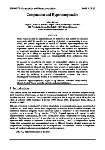
The SOFDs involved in the second order norm of an extra-ordinary CCSS patch (see eq. (2)) can be classified into two groups: group I and group II. Group I contains those SOFDs that involve vertices in the vicinity of the extra-ordinary vertex (see Figure 2(a)). These are the first 2n SOFDs in (2). Group II contains the remaining SOFDs, i.e., SOFDs that involve vertices in the vicinity of the other three vertices of S (see Figure 2(b)). These are the last 10 SOFDs in (2). It is easy to see that the convergence rate of the SOFDs in group II is the same as the regular case, i.e., 1/4 [3]. Therefore, to study properties of the second order norm M , it is sufficient to study norms of the SOFDs in group I. 2
3
2n+8
2n+1 . . .
11
2 3
1
10
8
4
2n+7
S
1 9
6
4
5
7 8
2n+6
S 6
5
2n+4
7
2n+5
(a)
2n+3
2n+2
(b)
Fig. 2. (a) Vicinity of the extra-ordinary point. (b) Vicinity of the other three vertices of S.
3.1
Matrix Based Rate of Convergence
The second order norm of S = S00 can be put in matrix form as follows: M = �AP�∞ where A is a 2n ∗ (2n + 1) matrix 2 −1 � �2 0
� � � � �2 A=� 0 � � 0 � � � � 0
0 0 0 −1
0 0 −1 2 −1 0 0 −1 2 0
0
0
�
0 −1 0 0 · · · 0 0 0 0 0 −1 · · · 0 0 � � � .. � . � � 0 0 0 0 · · · −1 0 � � 0 0 0 0 · · · 0 −1 � � −1 0 0 0 · · · 0 0 � � .. � � . 0 0 0 0 · · · 2 −1
Matrix Based Subdivision Depth Computation
549
and P is a control point vector P = [V1 , V2 , V3 , . . . , V2n+1 ]T . A is called the second order norm matrix for extra-ordinary CCSS patches. If i levels of Catmull-Clark subdivision are performed on the control mesh of S = S00 then, following the notation of Section 2, we have an extra-ordinary subpatch Si0 whose second order norm can be expressed as: � � Mi = �AΛi P�∞ where Λ is a subdivision matrix of dimension (2n + 1) ∗ (2n + 1). The function of Λ is to perform a subdivision step on the 2n + 1 control vertices around (and including) the extra-ordinary point (see Figure 2(a)). We are interested in � � knowing the relationship between �AP�∞ and �AΛi P�∞ . We need the following important result for AΛi . The proof of this result is shown in [2]. Lemma 4: AΛi = AΛi A+ A, where A+ is the pseudo-inverse matrix of A. With this lemma, we have �AΛi P�∞ �AP�∞
=
�AΛi A+ AP�∞ �AP�∞
≤
�AΛi A+ �∞ �AP�∞ �AP�∞
� � = �AΛi A+ �∞
� � Use ri to represent �AΛi A+ �∞ . Then we have the following recurrence formula for ri � i +� � � ri ≡ � A �∞� = �AΛi−1 A+ AΛA+ �∞ �AΛi−1 (4) ≤ �AΛ A+ �∞ �AΛA+ �∞ = ri−1 r1 where r0 = 1. Hence, we have the following lemma on the convergence rate of second order norm of an extra-ordinary CCSS patch. Lemma 5: The second order norm of an extra-ordinary CCSS patch satisfies the following inquality: (5) Mi ≤ ri M0 � i +� where ri = �AΛ A � and ri satisfies the recurrence formula (4). ∞
The recurrence formula (4) shows that ri in (5) can be replaced with r1i . However, experiment data show that, while the convergence rate changes by a constant ratio in most of the cases, there is a significant difference between r2 and r1 . The value of r2 is smaller than r12 by a significant gap. Hence, if we use r1i for ri in (5), we would end up with a bigger subdivision depth for a given error tolerance. A better choice is to use r2 to bound ri , as follows. j r2 , i = 2j ri ≤ (6) i = 2j + 1 r1 r2j , 3.2
Distance Evaluation
Following (12) and (13) of [4], the distance between the extra-ordinary CCSS patch S(u, v) and its control mesh L(u, v) can be expressed as
550
G. Chen and F. Cheng
m−2 �L(u, v) − S(u, v)� ≤ k=0 �Lk0 (uk , vk ) − Lk+1 (uk+1 , vk+1 )� 0 m m +�Lm−1 (um−1 , vm−1 ) − Lm 0 b (um , vm )� + �Lb (um , vm ) − Sb (um , vm )�
(7)
where um ,vm and b are defined in [4]. By applying Lemma 5, Lemma 6 and Lemma 1 of [4] on the first, second and third terms of the right hand side of the above inequality, respectively, we get
�
�L(u, v) − S(u, v)� ≤ c m−2 Mk + 14 Mm−1 + 13 Mm k=0 �m−2 ≤ M0 (c k=0 rk + 14 rm−1 + 13 rm )
where c = 1/ min{n, 8}. The last part of the above inequality follows from Lemma 2. Consequently, through a simple algebra, we have � 1−r j 1−r j−1 r r j−1 rj M0 [c( 1−r22 + 1−r2 2 r1 ) + 1 42 + 32 ], if m = 2j �L(u, v) − S(u, v)� ≤ 1−r j 1−r j rj r rj if m = 2j + 1 M0 [c( 1−r22 + 1−r22 r1 ) + 42 + 13 2 ], It can be easily proved that the maximum occurs at m = ∞. Hence, we have the following lemma. Lemma 6: The maximum of �L(u, v)−S(u, v)� satisfies the following inequality �L(u, v) − S(u, v)� ≤
M0 1 + r1 min{n, 8} 1 − r2
where ri = �AΛi A+ �∞ and M = M0 is the second order norm of the extraordinary patch S(u, v). 3.3
Subdivision Depth Computation
Lemma 6 can also be used to evaluate the distance between a level-i control mesh and the extra-ordinary patch S(u, v) for any i > 0. This is because the distance between a level-i control mesh and the surface patch S(u, v) is dominated by the distance between the level-i extra-ordinary subpatch and the corresponding control mesh which, accoriding to Lemma 6, is �Li (u, v) − S(u, v)� ≤
1 + r1 Mi min{n, 8} 1 − r2
where Mi is the second order norm of S(u, v)’s level-i control mesh, Mi . Hence, if the right side of the above inequality is smaller than a given error tolerance �, then the distance between S(u, v) and the level-i control mesh is smaller than �. Consequently, we have the following subdivision depth computation theorem for extra-ordinary CCSS patches. Theorem 7: Given an extra-ordinary surface patch S(u, v) and an error tolerance �, if i ≡ min{2l, 2k + 1} levels of subdivision are iteratively performed on the control mesh of S(u, v), where
Matrix Based Subdivision Depth Computation
551
1+r1 M0 1 l = �log r1 ( min{n,8} 1−r2 � ) , 2
1+r1 M0 r1 k = �log r1 ( min{n,8} 1−r2 � ) 2
with ri = �AΛi A+ �∞ and M0 being the second order norm of S(u, v), then the distance between S(u, v) and the level-i control mesh is smaller than �.
4
Examples
The new subdivision depth technique has been inplemented in C++ on the Windows platform to compare its performance with the previous approach. MatLab is used for both numerical and symbolic computation of ri in the implementation. Table 1 shows the comparison results of the previous technique, Theorem 3, with the new technique, Theorem 7. Two error tolerances 0.01 and 0.001 are considered and the second order norm M0 is assumed to be 2. For each error tolerance, we consider five different valences: 3, 5, 6, 7 and 8 for the extra-ordinary vertex. As can be seen from the table, the new technique has a 30% improvement over the previous technique in most of the cases. Hence, the new technique indeed improves the previous technique significantly. To show that the rates of convergence are indeed difference between r1 and r2 , their values from several typical extra-ordinary CCSS patches are also included in Table 1. Note that when we compare r1 and r2 , the value of r1 should be squared first. Table 1. Comparison between the old and the new technique � = 0.01 N Old New 3 14 9 5 16 11 6 19 16 7 23 14 8 37 27
5
� = 0.001 Old New 19 12 23 16 27 22 33 22 49 33
convergence rate r1 r2 0.6667 0.2917 0.7200 0.4016 0.8889 0.5098 0.8010 0.5121 1.0078 0.5691
Conclusions
A new subdivision depth computation technique for extra-ordinary CCSS patches is presented. The computation process is performed on matrix representation of the second order norm, which gives us a better bound of the convergence rate and, consequently, a tighter subdivision depth for a given error tolerance. Test results show that the new technique improves the previous technique by about 30% in most of the cases. This is a significant result because of the exponential nature of the subdivision process. Acknowledgement. Reserach work of the authors is supported by NSF under grant DMS-0310645 and DMI-0422126.
552
G. Chen and F. Cheng
References 1. Catmull E, Clark J, Recursively Generated B-spline Surfaces on Arbitrary Topological Meshes, Computer-Aided Design 10, 6, 350-355, 1978. 2. Chen G, Cheng F, Matrix based Subdivision Depth Computation for Extra-Ordinary Catmull-Clark Subdivision Surface Patches (complete version), http://www.cs.uky.edu/∼cheng/PUBL/ sub depth 3.pdf 3. Cheng F, Yong J, Subdivision Depth Computation for Catmull-Clark Subdivision Surfaces, Computer Aided Design & Applications 3, 1-4, 2006. 4. Cheng F, Chen G, Yong J, Subdivision Depth Computation for Extra-Ordinary Catmull-Clark Subdivision Surface Patches, to appear in Lecture Notes in Computer Science, Springer, 2006. 5. Halstead M, Kass M, DeRose T, Efficient, Fair Interpolation Using Catmull-Clark Surfaces, Proceedings of SIGGRAPH 1993, 35-44. 6. Lutterkort D, Peters J, Tight linear envelopes for splines, Numerische Mathematik 89, 4, 735-748, 2001. 7. Stam J, Exact Evaluation of Catmull-Clark Subdivision Surfaces at Arbitrary Parameter Values, Proceedings of SIGGRAPH 1998, 395-404.