Matrix Functions of Exponential Order - Semantic Scholar

Applied Mathematics, 2013, 4, 1260-1268 http://dx.doi.org/10.4236/am.2013.49170 Published Online September 2013 (http://www.scirp.org/journal/am)

Matrix Functions of Exponential Order Mithat Idemen Engineering Faculty, Okan University, Istanbul, Turkey Email: [email protected] Received May 31, 2013; revised June 30, 2013; accepted July 7, 2013 Copyright © 2013 Mithat Idemen. This is an open access article distributed under the Creative Commons Attribution License, which permits unrestricted use, distribution, and reproduction in any medium, provided the original work is properly cited.

ABSTRACT Both the theoretical and practical investigations of various dynamical systems need to extend the definitions of various functions defined on the real axis to the set of matrices. To this end one uses mainly three methods which are based on 1) the Jordan canonical forms, 2) the polynomial interpolation, and 3) the Cauchy integral formula. All these methods give the same result, say g(A), when they are applicable to given function g(t) and matrix A. But, unfortunately, each of them puts certain restrictions on g(t) and/or A, and needs tedious computations to find explicit exact expressions when the eigen-values of A are not simple. The aim of the present paper is to give an alternate method which is more logical, simple and applicable to all functions (continuous or discontinuous) of exponential order. It is based on the two-sided Laplace transform and analytical continuation concepts, and gives the result as a linear combination of certain n matrices determined only through A. Here n stands for the order of A. The coefficients taking place in the combination in question are given through the analytical continuation of g(t) (and its derivatives if A has multiple eigen-values) to the set of eigen-values of A (numerical computation of inverse transforms is not needed). Some illustrative examples show the effectiveness of the method. Keywords: Matrix; Matrix Functions; Analytical Continuation; Laplace Transform

1. Introduction For many theoretical and practical applications one needs to extend the definitions of functions defined on the real axis to the set of matrices. The history of the subject goes back to the second half of the nineteenth century when Cayley, who is the main instigator of the modern notation and terminology, introduced the concept of the square-root of a matrix A [1]. Since then a huge work has been devoted to the definitions, numerical computations and practical applications of the matrix functions. A rather detailed history (including a large reference list) and important results (especially those concerning the numerical computation techniques) are extensively discussed in the book by Higham [2]. So, we eschew here of making a review of the historical development and giving a large reference list. To extend the definition of a scalar function g(t), defined for t   , to the set of matrices, one starts from an explicit expression of g(t), which can be continued analytically into the complex plane C , and replaces there t by A. If the result is meaningful as a matrix, then it is defined to be g(A). Before going into further detail, it is worthwhile to clarify the meaning of the word “defined” appearing in the expression of “defined for Copyright © 2013 SciRes.

t   ”. It is especially important when g(t) consists of a multi-valued inverse function. To this end consider, for example, the square-root function g(t) = t1/2. Its definition requires, first of all, a cut connecting the branch point t = 0 to the other branch point t =  in the complex plane C . Then, by choosing one of its possible values at a given point, for example g(1), one defines it completely. The result consists of a well-defined branch of the square-root function. If one replaces t in this expression by A, then one gets a (unique) matrix to be denoted by A1/2. This matrix satisfies the equation X2 = A which may have many solutions denoted also by A1/2. The above-mentioned function g(A), which consists merely of the extension of the above-mentioned well-defined branch of the square-root function, can not permit us to find all these solutions. For example the equation X2 = I, where I denotes the unit 2 × 2 matrix, has infinitely many solutions given by cos  X  sin 

sin   ,  cos  

where  stands for any complex angle. All these matrices are defined to be the square-root I . But the abovementioned matrix g(A) gives only one of them, namely I AM

M. IDEMEN

or (−I). The known classical methods used in this context are grouped as follows (see [2], Sections 1, 2): 1) Methods based on the Jordan canonical formula; 2) Methods based on the Hermite interpolation formula; 3) Methods based on the Cauchy integral formula. All these methods are applicable when the function g(t), defined on the real axis, can be analytically continued into a domain of the complex-plane, which involves the spectrum of the matrix A (see def. 1.2 and def. 1.4 in [2]). Consider, for example, the Heaviside unit step function H(t) defined on the real axis by t0 1,  H  t   1 2, t  0 0, t  0. 

(1a)

z  0 z  0

(1b)

z  0.

Notice that (1a) and (1b) can also be obtained by computing the improper integral  1 d H  z  z  2 2  , 2π    z 2 (1c) where the bar on the integral sign stands for the Cauchy principal value. From (1b) one concludes that the seemingly general and elegant method 3), which is based on the Cauchy integral 1 g  A   1    I  A  d , 2πi C

(2)

where C stands for a closed contour such that the domain bounded by C involves all the eigen-values of A and the function g(z) is regular there, can not be applicable to Copyright © 2013 SciRes.

find H(A) (and other functions expressible through H(t)) when A has eigen-values having both positive and negative real parts. As to the methods 1) and 2), they need, in general, some tedious and cumbersome computations if A has multiple eigen-values. In the present note we will consider the case when the function g(t), defined on the real axis, is of the exponential order at both t = + and t = −, and give a new method which seems to be more logical and effective especially when the matrix A has multiple eigen-values. It gives the result as a linear combination of n matrices determined only by the matrix A. To this end we consider the Laplace transforms of g(t) on the right and left halves of the real axis, namely: 

gˆ   s      g   g  t  e st dt ,

It is obvious that the analytical continuation of H(t) into the complex z-plane, if it is exists, has the point z = 0 as a singular point. To reveal H(z), let us try to find its Taylor expansion about any point a > 0. This expansion is valid in the circle with center at the point z = a and radius equal to r = a. Since all the coefficients except the first one are equal to naught, one gets H(z)  1 at all points inside the circle in question. By letting a   one concludes that H(z) is regular in the right half-plane z > 0. If the above-mentioned Taylor expansion were made about a point a < 0, then one would get H(z)  0 for all z with z < 0. This shows that H(z) is a sectionally regular (holomorphic) function (see [3], Section 2.15). On the basis of the Plemelj-Sokhotiskii formulas (see [3], Section 2.17), for the points on the imaginary axis one writes H = 1/2, which yields 1,  H  z   1 2, 0, 

1261

(3a)

0 0

gˆ   s      g 

 g t  e

 st

(3b)

dt



and write [4] g t   1 2πi

 ts  ts L gˆ  s  e ds  2π1 i  gˆ  s  e ds, 

L

t   ,   .

(3c)

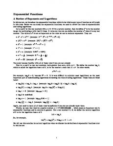
If the orders of the function g(t) for t   and t  (−) are c+ and c−, respectively, then the function gˆ   s  is a regular function of s in the right-half plane s  c  and the integration path L+ appearing in (3c) consists of any vertical straight-line located in this halfplane (see Figure 1). Similarly, gˆ   s  is regular in the half-plane s  c  and the integration path L− is any vertical straight-line in this half-plane (if c+ < c−, then one can assume L  L ). Furthermore, if g(t) as well as its derivatives up to the order (m-1) are all naught at t = 0, i.e. when g  0  g   0    g 

m 1

 0  0 ,

(4a)

then one has s

L−

c−

O

L+

c+

s

Figure 1. Regularity domains of gˆ   s  and the integration lines L when c− < c+. AM

M. IDEMEN

1262

   s

 g 

m

m

gˆ   s 

(4b)

and

   s

 g 

m

m

gˆ   s  ,

(4c)

which yield inversely 1 2πi

 m ts L gˆ  s  s e ds 

 1 2πi

t   ,   .

 gˆ  s  s

e ds  g  m   t  ,

m ts

L

(4d)

It is worthwhile to remark here that the formula (4d) m permits us to compute g    t  only at points on the real axis although g(t) and its derivatives are defined in (or can be continued analytically into) the complex t-plane. Therefore, when the point t is replaced by a complex   C , in what follows we will replace the left hand side m of (4d) by the analytical continuation of g    t  to the point  and write 1 2πi

m s  L gˆ  s  s e ds 

 1 2πi

 m m s   gˆ  s  s e ds  g    ,

L

  C .

2. Basic Results In what follows we will denote a square matrix A of entries ajk by A = [ajk]. Here the first and second indices show, respectively, the row and column where ajk is placed. The transpose of A will be indicated, as usual, by T a super index T such as AT   a jk  . The characteristic polynomial of A will be denoted by f    , i.e. f     det  A   I  . Theorem-1. Let A = [ajk] be an n  n matrix with characteristic polynomial f    . Then, 1) when all the zeros of f    , say 1 , , n , are distinct, one has n

exp  At    Γ0  e λα t

g  A  1 2πi

 As  As 1 L gˆ  s  e ds  2 π i  gˆ  s  e ds. 

(5)



with Γ0



Copyright © 2013 SciRes.

given by T

   f     ,  f       a jk  1

Γ0    

(6b)

2) when f    has p distinct zeros, say 1 , ,  p , with multiplicities m1 , , m p , respectively, one has exp  At  p



   m1t m 1   m 2t m  2     0  1





Γk    





with the matrices Γk

L

Thus the computation of g(A) becomes reduced to the computation of exp{At}. As we will see later on, the latter consists of a linear combination of certain constant matrices j ( j  1, , n = order of A). Hence g(A) will also be a linear combination of these j’s for every g(t). It is important to notice that to compute the coefficients in the combinations in question we will never need to compute the transform functions gˆ   s  as well as the integrals of the form (5) if the analytical continuation of m g    t  is known at the eigen-values of A (see the examples to be given in Section 4). These points constitute the essential properties of the definition (5): 1) It unifies the definition of g(A) for all functions g(t) of exponential order; 2) It gives an expression of g(A) in terms of certain matrices which take place in the expression of exp(At) and are determined only by A; 3) It reduces the computation of g(A) to the computation of exp(At) together with some scalar constants to be determined in terms of g(t) (and its derivatives when A has multiple eigen-values) at the eigen-values of A. The details are given in the theorems that follow.

(6a)

α 1

(4e) The formulas (3c), (4d) and (4e) will be the basis of our approach. Let A be a square matrix of dimensions n  n. We will define g(A) by replacing t in (3c) by A, namely:



 k  0,, ma  1

e

 t

(6c)

given by

1 k !  m  1  k  !

 m 1 k   d m 1 k  ds

  s   m  f s 

T (6d)       . f s    a    jk    s   

Theorem-2. Let A = [ajk] be an nn matrix while g(z), defined in the complex z-plane, is regular at all the eigenvalues of A and its restriction to the real axis is of exponential order at both t = + and t = −. If all the eigenvalues of A, say 1 , , n , are distinct, then one has n

g  A    g    Γ0  . 

(7)

 1

Here Γ0   a  1, , n  stands for the matrix taking place in the expression of exp{At}. Theorem-3. Let A = [ajk] be an n  n regular matrix which has p distinct eigen-values 1 , ,  p with multiplicities m1 , , m p , respectively, while g(z), defined in the complex z-plane, is regular at all the eigen-values of A and its restriction to the real axis is of exponential order at both t = + and t = −. Let the non-zero matrices taking place in the expression of exp{At} be  Γk   a  1, , p; k  0, , K  . Then one has 

AM

M. IDEMEN p



g  A   A N  Γm1G   1



m 1

    Γm2G m 2       Γ0 G   ,

where N stands for an integer such that G  t   t N g  t  and its derivatives up to the order (K-1) are all naught at t = 0. Before going into detail of proofs of the above-mentioned theorems, it is worthwhile to draw the attention to the fact that theorems 2 and 3 give the matrix function  g(A) as a combination of the n matrices Γk  which appear in the expression of exp(At). They are the same (invariant) for all g(t). Proof of theorem-1. Our basic matrix function exp{At} is defined, as usual, through the infinite series exp  at   1  at 

f s 

 1   2πi

T    st  f s     e    a jk   s  . 

1

 gˆ   s  e s ds  .  L

s   gˆ  s  e ds  2πi  

L

A N g  A    cm 1Γm1  cm  2 Γm 2    c0  Γ0  1



(13)

(14)

has multiple non-zero eigen-values and define G  t   t N g  t  where the integer N will be determined appropriately later on. If in (5) one replaces g(t) by G(t) and exp{As} by (6c), then we get

If all the eigen-values are real, then (3c) reduces (14) to (7). When some or all of the eigen-values are complex, we replace (3c) by (4e) with m = 0 and arrive again (7). Proof of theorem-3. Now consider the case when A



(12)

Proof of theorem-2. When the eigen-values of A are all simple, in (5) one replaces exp(As) by its expression given in (6a) and obtains

It is obvious that the derivatives in (13) yields a polynomial in t of degree  m  1 . Hence the final expression of exp(At) can be arranged as what is given in (6c).

p

(11)

Here the integration line L is any vertical straight-line such that all the eigen-values of A are located in the left side of L. If the eigen-values are all simple, then the integral in (12) is computed by residues and gives (6a). When some of the eigen-values are multiple, as stated in theorem-1b, the residue method gives

 d m 1   s   m 1   m 1   1 !  m f s d s      1   

 1

(10)

T

p

g  A   

.

  f  s   ts exp  At    1  1  e ds. 2πi L f  s    a jk 

exp  At   

T

... ... ... ann  s

Thus (9) yields

(9)

   f      f      a jk 

... an 2

 f  s  , j , k  1, 2, , n. 1 f  s   a jk

It is obvious that X(t) defined as above is the unique solution to the differential equation X'  t   AX  t  under the initial condition X(0) = I. Hence, by applying the Laplace transform to this equation one gets 1 Xˆ  s     A – sI  which permits us to write

1

... an 1

a1n a2 n

1

1 22 A t    X  t  , t  . 2!

n

a11  s a12 ... a21 a22  s ...

Then the entry of the inverse matrix  A  sI  , which is placed at the k-th row and j-th column, can be computed through the polynomial f  s  as follows:

1 22 a t  , t   2!

1 exp  At    1   A  sI  ets ds. 2πi L

(8)

Let the characteristic polynomial of A be f  s  :

by replacing there the scalar constant a by the square matrix A, namely: exp  At   I  At 

1263











,

(15a)

where ck   

Copyright © 2013 SciRes.

1 1 Gˆ   s  s k e s ds  Gˆ   s  s k e s ds 2πi L 2πi L

(15b)

AM

M. IDEMEN

1264

with   1, , p and k  0, , ma  1. Remark that some  of the coefficients Γk  may be equal to naught (see ex.-2). Let the largest sub-index k be K for which one has  Γk   0 . Then, by considering the requirements in (4a), we will choose the integer N such that G(t) and its derivatives up to the order (K-1) are all naught for t = 0. In this case all terms existing in (15b) are computed through (4d) or (4e) and give (8).

3. A Corollary (Cayley-Hamilton Theorem) Let g(t) be the characteristic polynomial of A (i.e. g(t)  f(t)). In this case all the terms taking place in (7) or (8) are equal to zero. When the eigen-values are all simple, from (7) one gets directly f(A) = 0, which is valid for both regular and singular matrices. In the case of multiple eigen-values, (8) gives f(A) = 0 if A is not singular. We remark that the Cayley-Hamilton theorem is correct for all matrices. We will use this theorem to compute the factor A−N taking place in the formula (8) (see ex.-2).

4. Some Illustrative Examples In order to show the application and effectiveness of the method, in what follows we will consider some simple examples. Ex.-1 As a first example consider the case where A is as follows:  8 12 2  A   3 4 1  .  1 2 2 

One can easily check that A has a triple eigen-value  = 2. Therefore the theorems 1b and 3 are applicable directly for all functions of exponential order. The quanti-

ties p and m mentioned in those theorems are: p = 1, m1 = 3. On the other hand from 8 f     3 1

12 4   2

2 1     2 2

3

one computes  2  2  6 12  20 4  2  T      2   10  14  2   a f       5  3  jk   2 4  2  2  4  4  

which gives (see (6c) and (6d))





exp  At   Γ 2t 2  Γ1t  Γ0 e2t

where  6 12 2   0  I , 1   3 6 1   1 2 0 

and  2 4 0 1 Γ 2   1 2 0  . 2  0 0 0 

Since 2  0, one has K = 2 which shows that the formula (8) is applicable with 0  N  2. For example, in order to find the expressions of A and sin A (with   2), one can choose N = 0 while A , sin A , sin A , sin 3 A , arcsinA etc. needs N = 1. To compute cosA, logA, cos A , signA and arcosA one has to choose N = 2. To check the formulas, we would like to compute first An (n = integer  2) through the formula (7) which gives

 2n2  n  n  1  12n  4  2n 1  n  n  1  12n  2n n    An  n  n  1 2n2 Γ 2  n  2n1 Γ1  2n Γ 0   2n 3  n  n  1  12n  2n 2  n  n  1  12n  4  2n 1 n  .    n 1 n n  2 n 2 n 2  

Thus for n = 2 one gets  30 52 8   A2   13 22 4  .    4 8 4 

Notice that by a direct multiplication of A with itself one gets the same result. Similarly, one gets also 4 4   g  t   3 t  A 3 A   t 4 3  Γ 2  t 4 3  Γ1  t 4 3Γ 0    2 3 Γ 2   1 3Γ1   4 3 I ,  3  2 3   t 2 9

 

Copyright © 2013 SciRes.

 

AM

M. IDEMEN

1265

    g  t   log  xt   A2 log  Ax    t 2 log  xt  Γ 2  t 2 log  xt  Γ1  t 2 log  xt  Γ 0    t 2









 2 log  2 x   3 Γ 2  4 log  2 x   2 Γ1  4 log  2 x  I ,

 

g  t   cos x t  A2 cos x2     2   cos 2  





 



7x sin 2

2x 

g  t   sin x t  Asin  3x  cos 4 2

 





 

 2 x  Γ 2  4 cos 







   





2 x  2 x sin



  

 



2 x Γ1  4cos





2x I ,

    A x   t sin x t Γ2  t sin x t Γ1  t sin x t Γ0    t 2



2x 

 

    A x   t 2 cos x t Γ 2  t 2 cos x t Γ1  t 2 cos x t Γ 0    t 2



x2 sin 4

  x 2 x  Γ2   cos  2 









2 x  sin



 



 2 x  Γ1  2sin 





2x I ,

 30 52 8 g  t   signt  A signA  2Γ 2  4Γ1  4Γ 0   13 22 4   A2  signA  I .  4 8 4  2

Remark that for different branches of t , 3 t and log  xt  one gets different expressions for 3 A , log  Ax  , cos



Ax



and sin



Ax



taking place in the formula (8) can be computed rather easily by using the Cayley-Hamilton theorem as follows:  6 20 4  1 A   5 14 2  , 8  2 4 4 

(see Section 5

and theorem-4). Finally, let us consider the branches of the inverse trigonometric functions g(t) = arcsint and h(t) = arccost which map the t-plane cut as shown in Figure 2 into the regions in the g- and h-planes shown in Figures 3 and 4 (the so-called principal branches of these functions!). For the first function we have to choose N = 1 while the second one needs N = 2. The matrices A−1 and A−2

1

 56 144 32  1  36 88 16  . A  64  32 16   16 2

Thus, by starting from G  t   tarcsint and H  t   t 2 arccost one gets from (8)

8

16 0 

 20

40

 0

0

0 

 4

8

    2  arcsin A  4 8 0   10 20 8  24 

8  4   4 0 

 6 20 4   5 14 2    4 4   2

and arccos A 

 32 64 0   64 128 32   56 144 32         88 16   16 32 0   16  32 64 16   16  36  0  16 32 0   16 0 0  32 16 

  8 3  64

with

  arcsin2,   arccos2,   1

3 .

It is an interesting exercise to check that arcsin A  arccos A   0   I   I 

π I. 2

Ex.-2 Now consider the case where A is as follows: Copyright © 2013 SciRes.

7 0 4 A   8 3 8  .  8 0 5 In this case one has f         1   3 , 2

which shows again that the theorems 1b and 3 are appliAM

M. IDEMEN

1266

e At  e t Γ0   e3t Γ0  . 1

2

Since K = 0, (8) is applicable with N = 0 and gives, for example, B− B+

C2



C1

A− A+

1

−1

signA  sign  1  Γ0   sign  2  Γ1   sign  2  Γ0  1

t

Figure 2. Complex plane-t cut along the lines (−) < t < −1 and 1 < t < .

1

2

3 0 2 4 1 4    4 0 3

and H  A   H  1  Γ0   H   2  Γ1   H  2  Γ0   Γ0 

A−

C1

−/2

/2

g

2

A+

Figure 3. Mapping of the t-plane into the g-plane through the principal branch of the function g = arcsint.

A+

2

2

By direct multiplication of these matrices by themselves one gets

signA B+

2

2 0 1   2 1 2  .  2 0 1

 arcsin

C2

2

 Γ0   Γ0 

1

B−

2

 I , H  A   H  A  , 2

which are the basic properties for the original functions signt and H(t). Similarly, one gets also

B+

 2   arcsin A   2  2  2  2 

    2   2  0 2   

 2   arccos A   2  2  2  2

    2  2  0 2   

0

and C1

C2 

O arccos  A−

h

B−

0

with

  arcsin  1 ,   arcsin3,

Figure 4. Mapping of the t-plane into the h-plane through the principal branch of the function h = arccost.

  arcos  1 ,   arccos3 .

cable with p = 2, 1 = −1, 2 = 3, m1 = 1 and m2 = 2. From the expression of f() one gets easily

Here the functions arcsin t  g  t  and arccos t  h  t  consist of the functions considered in the example1 above. One can easily check that

1

Γ0

 1 0 1 2 0 1    2    2 0 2  , Γ 0   2 1 2   2 0 2   2 0 1

and  2

Γ1

0 0 0  0 0 0   0 . 0 0 0 

Therefore from (6c) and (8) we write Copyright © 2013 SciRes.

sin  arcsinA   A and arcsin A  arccos A 

π I, 2

which are the basic properties for the original functions arcsint and arccost. Ex.-3 Finally, we want to give an example with complex-valued eigen-values. To this end consider the case where  a b  A  b a  AM

M. IDEMEN

1267

signA  sign  a  ib  Γ0   sign  a  ib  Γ0 

with any real a and b. In this case one has

1

1  a  ib, 2  a  ib

 Γ01  Γ02   I , if a  0  1   2   Γ0  Γ0   I , if a  0 0, if a  0 

 1 i 1  i  1 2 , Γ0   1  and Γ0   1  . 2  i 1 2  i 1 

Thus, for the following functions one writes

2

and

1  1  i arcsin  a  ib   arcsin  a  ib   2 arcsin  a  ib   arcsin  a  ib  2 arcsin A   . 1   i arcsin  a  ib   arcsin  a  ib  1 arcsin  a  b   arcsin  a  ib    2  2

Here arcsint stands for the function defined in ex.-1 above. It is interesting to check that

signA

 I if a  0, sin  arcsinA   A

2

5. Inverse Power of a Matrix From the example 1 considered above one observes that there are many inverse powers A1/m (= B) which correspond to a given matrix A through the relation Bm = A. The next lemma and theorem concern this case. Lemma. Let the values of the function g  t   t1 m , defined on a Riemann surface, at given p points 1 , 2 , ,  p be g   j   wjk   0 , k  1, , m . Then there is a Riemann surface such that on one of its sheets g(t) takes previously chosen values at the points 1 , 2 , ,  p , namely: g  j   wj

k 

with arbitrarily chosen

k j  1, 2, , m , j  1, 2, , p .

Proof. Let at the first r points (1  r < p) one has g   j   wj1 while at r 1 one wants to have q g  r 1   wr 1 , where q  2, , m is any number. Then, we define the new cut line as a spiral curve which starts from the branch point t = 0, encircles the points 1 , 2 , , r (see the Figure 4) and (q-1) times passes between the points r and r 1 . Thus the analytic con1 tinuation of g  1   w1  to j  j  2, , r  becomes q 1 w j while at r 1 it is equal to wr 1 . We continue this process to adjust also the values at the points r  2 , , n . k  Notice that when the super index kj + 1 in w j j11 is smaller

than kj, we can replace kj + 1 by (kj + 1 + m) because one k   k  m has w j j11  w j j11 . At the end we arrive at a plane cut

g  6   w6  , g  7   w7  , g  8   w8  . 4

4

5

Theorem-4. Let A be an n  n regular matrix with p different eigen-values 1  p  n  while m is an integer. Then there exist at least mp different matrices B such that Bm = A. Proof. Let the eigen-values of A be  j  j  1, , p  . Consider a Riemann surface which corresponds to the function g  t   t1 m and denote, on the k-th sheet of this Riemann surface, the values of the function g(t) at points 1m j by   j    

k 

 wj  ,  k  1, , m  . On the basis of k

the lemma, we can change the cut line appropriately such that the values of t1/m at the points  1 , 2 , ,  p  become equal to previously chosen values. For example,

 1 

1m

1

 w1  , 1

 2 

1m

 w2  , 3

 3 

1m

 w3  , 2

 4 

1m



p

w4 etc. Since these values can be arranged in m different forms, the right-hand side of (7) (or (8)) can have mp different values. This proves thorem-4. Ex. Let a  C and b  C any numbers which differ from zero. Then the matrix a2 0  A 2 0 b   

O

 





1





5

6



8

7 t

along an appropriate (spiral) curve joining the point t = 0 to t =  such that at the given points  1 , 2 , ,  p  the k  function g(t) has desired values w j j . For example on the Riemann sheet shown in Figure 5 one has g  1   w1  , g  2   w2  , , g  5   w5  , 1

Copyright © 2013 SciRes.

1

1

Figure 5. A cut appropriate for the particular case when r = 5 and q = 4.

AM

M. IDEMEN

1268

Vol. 148, 1858, pp. 17-37. doi:10.1098/rstl.1858.0002

has four square-roots given as follows:  a 0   a 0   a 0   a 0  , , . 0 b  , 0 b  0 b  0 b    

REFERENCES [1]

A. Cayley, “A Memoir on the Theory of Matrices,” Philosophical Transactions of the Royal Society of London,

Copyright © 2013 SciRes.

[2]

N. J. Higham, “Functions of Matrices: Theory and Computation,” Society for Industrial and Applied Mathematica (SIAM), Philadelphia, 2008.

[3]

N. I. Mushkhelishvili, “Singular Integral Equations,” P. Noordhoff Ltd., Holland, 1958.

[4]

E. C. Titchmarsh, “Introduction to the Theory of Fourier Integrals,” Chelsea Publishing Company, 1986, Chapter 1.3.

AM