Matrix Techniques for Modeling Ultrasonic Waves in ... - IEEE Xplore

IEEE TRANSACTIONS ON ULTRASONICS, FERROELECTRICS, AND FREQUENCY CONTROL, VOL. 42, NO. 4, JULY 1995

525

Matrix Techniques for Modeling Ultrasonic Waves in Multilayered Media Michael J. S. Lowe

Abstract— Research into ultrasonic NDE techniques for the inspection of multilayered structures relies strongly on the use of modeling tools which calculate dispersion curves and reflection and transmission spectra. These predictions are essential to enable the best inspection strategies to be identified and their sensitivities to be evaluated. General purpose multilayer modeling tools may be developed from a number of matrix formulations which have evolved in the latter half of this century and there is now a formidable number of publications on the subject. This paper presents a review of the main developments of the matrix techniques, and their use in response and modal models, with emphasis on ultrasonics applications.

I. INTRODUCTION

R

ESEARCH into the use of ultrasonics for nondestructive inspection frequently involves the study of the interaction of sound with multilayered plate structures. Important research areas include the detection of poor cohesion and adhesion in adhesive joints, the measurement of the elastic properties and thickness of sheet materials, including carbon fiber composites, the detection of damage in composites, and the inspection of surface and surface layer properties using acoustic microscopes. Inspection methods for such tasks can be considered broadly in two groups: response methods in which the reflection and transmission characteristics of the plate are examined (e.g., measurement of reflection coefficient), and modal methods which address the plate wave propagation properties of the system (e.g., measurement of Lamb wave velocity). The development of inspection techniques based on either approach requires the study of complicated wave mechanics and relies strongly on the use of predictive modeling tools to enable the best inspection strategies to be identified and their sensitivities to be evaluated. The modeling tools may be developed from matrix formulations which describe elastic waves in layered media with arbitrary numbers of layers. The formulations combine the theory of the dynamics of the continuum within each layer with the conditions for the interaction at the interfaces between layers. This results in a matrix description of the system in terms of its external boundaries: stresses and displacements at a free surface or incoming and outgoing wave amplitudes in an immersed plate. Both response and modal models may make use of the same matrix formulation, but involve different solutions. Response models calculate the amplitudes Manuscript received March 16, 1994; revised November 15, 1994. The author is with the Department of Mechanical Engineering, Imperial College of Science, Technology, and Medicine, Exhibition Road, London SW7 2BX, United Kingdom. IEEE Log Number 9409991.

and phases of reflected and transmitted infinite plane waves resulting from a given incident plane wave. Finite fields may then be studied by superposition of the infinite plane wave solutions. Modal models calculate the unforced properties of the system: the velocities and frequencies (dispersion curves) at which plate waves may travel along the plate. “True” (or “free”) waves travel without decay in amplitude. They can only exist in perfectly elastic materials and they do not leak energy into adjacent media. “Leaky” waves emit energy in the form of outgoing waves in the adjacent media and therefore they decay in amplitude as they travel. Waves may also decay if energy is dissipated in layers which have material damping properties. The matrix formulations have evolved in the latter half of this century and have featured in a large number of publications. Indeed there are currently two quite different approaches and many variants which are in accepted use. The purpose of this paper is to review the main developments of the techniques and their implementation in response and modal models. The paper is intended to benefit researchers who wish to develop predictive models or to make use of the formulations in analytical investigations. It therefore includes detailed descriptions of both the Transfer Matrix method (Thomson-Haskell) and the Global Matrix method. The emphasis throughout is on ultrasonics applications.

A. Historical Background The earliest theory for wave propagation in multilayered media was Lord Rayleigh’s derivation [1] in 1885 for waves travelling along the free surface of a semi-infinite elastic halfspace. The derivation yields a third order expression whose roots determine the velocity of the propagating surface wave. A generalization of the single interface problem was developed by Stoneley [2] in 1924 to describe waves travelling along the interface between two different elastic solids. Later studies addressed the conditions when these waves may travel without leaking into either of the solids (true modes) [3] and the existence of leaky modes [4]. In 1917 Lamb [5] added another interface to introduce the notion of a flat layer of finite thickness. His derivation was for plates in vacuum and the roots of his two equations, one for symmetric modes and one for antisymmetric modes, yield the well known Lamb wave dispersion curves. Love [6] showed that transverse modes, involving shearing motion in the plane of the layer, were also possible in layers of finite thickness. Discussions of these and other specific layer geometries may be found in [7]–[11].

0885–3010/95$04.00  1995 IEEE

526


The first derivation of equations for wave propagation in media consisting of arbitrary numbers of flat layers was published by Thomson [12] in 1950. He introduced a transfer matrix which described the displacements and stresses at the bottom of a layer with respect to those at the top of the layer. The matrices for any number of layers could be coupled to yield a single matrix for the complete system. Thus the displacements and stresses at the bottom of a multilayered system could be related to those at the top of the system. Modal or response solutions could then be found by application of the appropriate boundary conditions. A small error in his derivation was corrected by Haskell [13]. The theory was developed for seismological applications where interest was in surface waves in media consisting of multiple different rock layers. Because the method involves the propagation of the boundary conditions from one boundary of the system to the other via matrix multiplications, it is also referred to as a “propagator matrix” method. Following Thomson’s work, and aided by the availability of digital computers, there was an increase in investigations into the modeling of wave propagation in multilayered media, almost entirely for seismological applications. The models were demanding on computer resources which were rather limited at that time and consequently a number of publications, particularly during the 1960s, addressed the implementation of the transfer matrix method and the practicalities of solving the response equations or modal equations by computer with maximum efficiency [14]–[17]. A development of the theory which received significant attention was the modeling of waves whose amplitude decay with distance along the plate. This was important partly because of the damping properties of the Earth’s strata, but mainly because of the desire to model leaky wave modes in rock layers. These modes leak energy into adjacent media and their amplitudes thus decay as they propagate. Such solutions were not possible with the original theory and required the introduction of a real exponential factor in the wave equation, achieved by allowing either the frequency or the wavenumber to be generally complex [17]–[29]. An important problem arose during the early developments of the transfer matrix method, concerning the instability of the solution when layers of large thickness are present and high frequencies are being considered [30]. This has become problem” ( is frequency and is layer known as the “large thickness), and was the subject of much research effort for two decades. The cause of the problem is the poor conditioning of the propagator matrices due to a combination of both decaying and growing coefficients when inhomogeneous (evanescent) waves are present. This is well known but views differ as to the appropriate solution. Undoubtedly the answer is applicationdependent. One approach, first proposed by Dunkin [30] and later pursued by others in various forms [31]–[44], has been to retain the concept of transfer matrices but to rearrange the equations such that they do not become ill-conditioned. Such a technique retains the advantage of a small system matrix but loses the conceptual simplicity of the Thomson-Haskell formulation. An alternative, and quite different, approach is to employ a “Global matrix,” proposed originally by Knopoff

[45], in which a large single matrix is assembled, consisting of all of the equations for all of the layers [15], [46]–[53]. This technique is robust and can be implemented simply but may be relatively slow to compute when there are many layers and the matrix is large. Response solutions of the matrix equations yield the steady state plane wave response of a multilayered plate to plane wave excitation. In the early history of the techniques, the developers were mainly concerned with simulating the response to finite duration excitation at a point (or points) within a layer. This response to a point source can be predicted by performing an integration of the multiple plane wave solutions over wavenumber and frequency [19], [23], [24], [29], [49], [54]–[57]. In order to account for attenuating wave modes, the wavenumber integration may be performed using Green’s function along a path in the complex wavenumber plane. More recently, in ultrasonics applications, researchers have been interested in simulating the response of multilayered plates to finite sized transducers. Again this can be achieved by integrating over wavenumber and frequency [52], [58]–[60]. Modal solutions of the matrix equations describe the wave propagation properties of a multilayered plate, being the velocities, frequencies and rates of decay of waves which may propagate along the plate. A solution requires the determination of the roots of a characteristic function, found from the layer matrices and dependent on wavenumber and frequency. The modal solution is somewhat more difficult than the plane wave response calculations, and is particularly challenging if decaying modes are to be found, when the wavenumber (or frequency) is complex. Modal models have been used extensively in research reported in both seismological and ultrasonics applications. However, in the literature which discusses solution strategies [13], [14], [28], [35], [40], [46], [51], [53], [61]–[64], comparatively little detail is given and the majority of implementations are limited to true modes. Matrix techniques have been popular for the modeling of ultrasound in multilayered plates for about the last two decades. The ultrasonics research community has made extensive use of the early developments but has also contributed to the evolution of the techniques, as evidenced by a significant number of the references cited above. Currently, major areas of the development of these techniques in ultrasonics are in viscoelastic and anisotropic media (particularly composites) [42]–[44], [65]–[75]. B. Outline Paper In the majority of model studies it is not necessary to consider material damping, leaky plate wave modes or high frequency-thickness products (e.g., above 10 MHz-mm in metal plates). For such applications the Transfer Matrix method, which is intuitive and relatively simple, is perfectly satisfactory. The paper starts therefore, in Sections II and III, with the development of a Transfer Matrix formulation for response and modal solutions, limited to isotropic elastic materials and true plate wave modes. This is essentially a simple description of the Thomson-Haskell technique. Section IV reviews the major developments of the Transfer Matrix method: The extension of the theory to include material

LOWE: MATRIX TECHNIQUES FOR MODELING ULTRASONIC WAVES IN MULTILAYERED MEDIA

damping and leaky wave modes, the numerical instabilities encountered at high frequency-thicknesses and the variant reformulations of the Transfer Matrix method which have been proposed to restore its stability. Section V describes the Global Matrix method which is a quite different alternative to the Transfer Matrix method. It can incorporate the material damping and leaky mode developments and does not suffer from the numerical instability. Finally, Section VI introduces briefly the implementation of anisotropic layers, which are necessary for modeling multilayer fiber composites for example, and cylindrical layers which enable the models to include circular bars and tubular structures.

527

(2) where

and

are Lamé’s elastic stiffness constants and is the change in volume (dilatation)

of the element. Substitution yields the displacement equations of motion

II. FIELD EQUATIONS FOR PLANE WAVES IN FLAT ISOTROPIC ELASTIC LAYERS The field equations for the displacements and stresses in a flat isotropic elastic solid layer may be expressed as the superposition of the fields of four bulk waves within the layer. The approach therefore is to derive the field equations for bulk waves, which are solutions to the wave equation in an infinite medium, and then to introduce the boundary conditions at an interface between two layers (Snell’s law), so defining the rules for coupling between layers and for the superposition of the bulk waves. The analysis of the layers is restricted to two dimensions, with the imposition of plane strain and motion in the plane only. A. Plane Waves in an Infinite Elastic Solid The development of the equations of motion for an infinite elastic solid has been covered in many texts [10], [11], [76]. The usual approach, summarized here, is to start with an infinitesimal cubic element in an infinite elastic isotropic solid of density A Cartesian system is adopted, with and in the coordinate system displacements and By application of Newton’s second law, equilibrium requires that:

(1) where are the stress components acting on the faces of the cube and is time. These are the fundamental stress equations of motion for the medium. It will be more convenient if they are expressed in terms of displacements, by introducing the stress-strain and the strain-displacement equations:

(3) which may be expressed in the vector form: (4) where is the vector operator and is the scalar operator This equation cannot be integrated directly; a form of solution must be assumed and checked for suitability by differentiation and substitution. Here it is assumed that the wavefront is an infinite plane which is normal to the direction of propagation, as illustrated in Fig. 1. It is also assumed that, at any position in the propagation direction and at any instant in time, all displacements are uniform over the plane of the wavefront. This defines a homogeneous plane wave. For such assumptions there are two solutions, one for “longitudinal” waves and the other for “shear” waves (the “bulk waves”). The particle motion in longitudinal waves is entirely in the direction of propagation and the wave motion consists of change of volume (dilatation) only. The particle motion in shear waves is normal to the direction of propagation and the motion consists of rotation of the medium without change of volume. A convenient way of presenting the solutions in vector form is by the Helmholtz method [77], in which longitudinal are described by a scalar function and shear waves by a vector function whose direction is normal waves to both the direction of wave propagation and the direction of particle motion:

(5) and are the longitudinal and shear wave Here amplitudes, is the wavenumber vector and is the angular frequency. The wavenumber vector is in the direction of

528


plate boundaries are not considered. For plane strain there is direction no variation of any quantity in the Furthermore, as is usual in ultrasonics applications, the model is restricted to waves whose particle motion is entirely in the thus excluding Love [6] modes. The modeling plane of Love modes requires only minor changes to the derivations and may be pursued with the aid of the seismological literature where they have received considerably more attention [9], [17], [28], [61], [78]. From (7) the displacements of longitudinal and shear waves are now given by:

Fig. 1. Propagation of a plane wave in an infinite elastic medium, with wavenumber vector,k.

propagation of the wave and describes its wavelength and speed. Wavelength

Speed

(9)

(6)

The wavenumber is illustrated in Fig. 1. To generalize the expressions the amplitudes may be taken as complex quantities where is the phase of the wave at the spatial and temporal origin The displacement fields are given by the operations:

(7) where denotes the vector cross product. Substitution into the equation of motion (4) gives the wave speeds, in terms of the material properties: say say

(8)

where for completeness the expressions in terms of Young’s and Poisson’s ratio are included. modulus B. Plane Waves in a Two-Dimensional Space It is usually assumed in multilayered plate models that the wavelengths are significantly smaller than the width of the plate and of the wave fields and therefore that a plane strain analysis is valid. The coordinate system may then be reduced to the plane defined by the direction of propagation of the waves and the normal to the plate. For convenience here, the parallel to the plate and normal to plane is defined by the plate. Fig. 2 illustrates the coordinate system which will be used for the plate, although at this stage the layer interfaces and

in which the vector potential points in the plane. that all particle motion is in the

direction so

C. The Superposition of Plane Waves in a Layered Plate The development of a model for wave motion in multilayered plates is achieved by the superposition of longitudinal and shear bulk waves and the imposition of boundary conditions at the interfaces between the layers. At each interface, it is sufficient to assume eight waves: longitudinal and shear waves arriving from “above” the interface and leaving “below” and, similarly, longitudinal and shear the interface waves arriving from below the interface and leaving above the There are thus four waves in each layer interface of the multilayered plate (Fig. 2). Snell’s law requires that for interaction of the waves they must all share the same frequency direction at each interface. and spatial properties in the It follows that all displacement and stress equations have the same and the same component of wavenumber (the “plate wavenumber”), being the projection of the wavenumber of the bulk wave onto the interface. All field equations for all locations in all layers therefore contain the following factor, which is an invariant of the system: (10) This constrains the angles of incidence, transmission and reflection of homogeneous bulk waves in the layers according to their bulk wave velocities, by the relationship: (11) where and are the angles at which longitudinal and shear bulk waves propagate with respect to the normal to the


529

Fig. 2. Labeling system for multilayered plate.

layers ( direction). The invariant is the projection of direction and will be the the bulk wave velocities in the phase velocity of the propagating waves described by modal components of the bulk waves in each layer solutions. The may also be expressed, using (6) and (8), in terms of the plate and the bulk wave velocities for the material, wavenumber and : and for shear bulk waves: (12) Again the + and signs denote waves travelling in directions with positive (“downward”) and negative (“upward”) components, respectively. If is greater than then is real and the wave is homogeneous and travels at some nonzero angle with respect to the direction. If is less than then is entirely imaginary and the wave is inhomogeneous, or “evanescent,” propagating in the direction and decaying in amplitude in the direction. Thus the displacements and stresses at any location in a layer maybe found from the amplitudes of the bulk waves, using the field equations: For longitudinal bulk waves:

(13) The displacements and stresses at any location in a layer may therefore be found by summing the contributions due to the four wave components in the layer. For a multilayered system, the field quantities of interest are those which must be continuous at the interfaces: the two displacement components and the normal stress and the shear stress Making the substitutions for convenience,

(14)

530


and omitting the common factor, the field quantities in a layer are thus expressed by the matrix equation:

u1 u2 22 12

=

k1 g C g iBg 2ik1 2 C g

1

k1 g 0C g iB g 02ik1 2C g

C g

0k g 1

02ik 1

2

C g

0C g 0k

(16)

1

g 2ik1 2 C g

iBg

A(L+) A(L0) A(S+) A(S0)

which has its origin at its interface with for the first layer in order to avoid having an origin at Assume that the displacements and stresses are known at The amplitudes of the four waves at the the first interface, top of layer can now be found by inverting the matrix :

iB g

the displacements and stresses at At the second interface, the bottom of the layer can be found from the wave amplitudes in layer :

(15)

In summary, the matrix in (15) is the field matrix, describing the relationship between the wave amplitudes and the displacements and stresses at any location in any layer. Its coefficients the depend on the through-thickness position in the plate and material properties of the layer at this position the frequency and the invariant plate wavenumber The origin of the coordinate may be placed arbitrarily and may even be different for each layer because phase differences between layers can be accounted for by the phase of the complex wave amplitudes. The field matrix will be abbreviated here to III. THE TRANSFER MATRIX METHOD ELASTIC WAVES AND TRUE MODES

FOR

The Transfer Matrix method works by condensing the multilayered system into a set of four equations relating the boundary conditions at the first interface to the boundary conditions at the last interface. In the process, the equations for the intermediate interfaces are eliminated so that the fields in all of the layers of the plate are described solely in terms of the external boundary conditions. The basic principle of a transfer matrix description for layered media should be attributed to Thomson [12], who showed that the matrices could be used to describe the transmission of waves through an arbitrary number of layers. Haskell [13] subsequently corrected an error in Thomson’s paper and went on to show that the method could be used to find the modal solutions for surface waves. Fig. 2 shows the labeling system which will be used in the following discussion. A five layer system is illustrated as an example, consisting of a three layer plate with two semi-infinite half-spaces. The half-spaces are included here as layers, even if they are vacuum. The layers of the system and the interfaces, to Although the are labeled to orientation of the plate in space is arbitrary, it is convenient to refer to the layers and interfaces in terms of their vertical positions in a stack and to the top and bottom surfaces, as in the direction is defined as downwards, figure. Accordingly the from the top to the bottom of the plate. Each layer has its own origin, defined as the location of its top interface, except

(17)

The matrix product in this equation now relates the displacements and stresses between the top and bottom surfaces of a single layer and may be referred to as the layer matrix, which for layer is: (18) The inverted matrix may be expressed explicitly [13], [53], [70] and therefore it is possible to write out the coefficients of matrix, providing a useful basis for analytical studies. the The coefficients are:


(19) The displacements and stresses must be continuous across a “welded” interface between two layers. Therefore:

(20)

Clearly this process can be continued layer by layer for all subsequent layers, resulting in the equation:

531

The response solution gives the amplitudes and phases of steady state, fixed frequency, reflected and transmitted plane infinite waves. In many cases this is sufficient information for model studies. However, as mentioned in the introduction, it is also possible to make predictions of response which are finite in both space and time [52], [58]–[60] and thus simulate, for example, the finite-time signal which is received by a finitesized transducer. The finite spatial domain may be modeled by performing a Fourier angular (or plate wavenumber) decomposition of the finite field in front of the transmitting transducer into infinite plane wave components and then calculating an infinite plane wave solution for each component. The reflected or transmitted field may then be composed by summing the infinite plane wave solutions and the signal received by a finite transducer may be found by integrating the field over the face of the transducer. The finite time domain signal may be predicted by calculating the infinite or finite field responses over a range of frequencies and then performing an inverse Fourier transform to the time domain. B. Modal Solution for True Modes

(21)

where is the last layer ( in the example) and is the system matrix consisting of the matrix product of the layer matrices: (22) Finally, if a half-space is not vacuum, then it is useful to describe that boundary of the system in terms of the waves in the half-space rather than the displacements and stresses. Therefore, for the case in which both half-spaces are solids, the system equation is:

(23)

If both of the half-spaces are vacuum then a modal solution requires that the stresses must be zero at the extreme interfaces and as illustrated in Fig. 3(a). Now (21) may be written:

(24)

Expanding this equation for the two (zero) stress terms on the left-hand side gives: (25) where the two-by-two matrix is the bottom left sub-matrix of (rows 3 and 4 and columns 1 and 2). For this equation to be satisfied, the submatrix must be singular. Thus, defining the for the system: determinant as the characteristic function

A. Response Solution For an infinite plane wave response solution for a plate embedded in a solid, four of the eight wave amplitudes of (23) must be known, enabling the remaining four to be found by direct manipulation of the equation. Typically, one of the four incoming waves is assumed to have unit amplitude and the others to be zero. The plane wave reflection and transmission coefficients are then given by the amplitudes of the four outgoing waves. If the plate is immersed in a fluid then strictly speaking the equations must be rewritten to omit the possibility of shear waves in the fluid (also, if one of the layers of the plate system is a fluid [13]). However, a practical approach is to specify shear properties for the fluid such that the full set of equations for the solid media may be solved yet the shear motion in the fluid is negligible. This can be achieved by specifying a very low bulk shear velocity for the fluid, for example several orders of magnitude lower than the bulk longitudinal velocity [52].

(26) True modes may also travel in plate systems in which one or both of the half-spaces are not vacuum, but only under the condition that no energy leaks from the plate into the halfspaces. For this condition to be satisfied, any wave components and must be inhomogeneous so that in the half-spaces they may carry energy along the plate but are unable to carry and energy away from the extreme interfaces Taking the example of a plate system in which neither halfspace is vacuum, the characteristic function may be found from (23). The condition for true mode propagation is that the wave should exist without forcing; therefore that there should be no energy coming into the system, as illustrated in Fig. 3(b). Thus, the denoting the product of the three matrices in (23) as for this system is: characteristic function (27)

532


(a)

(b) Fig. 3.

Boundary conditions for modal solutions in plates. (a) Plate in vacuum. (b) Plate in solid or liquid semi-infinite half-spaces.

Solutions of the characteristic functions can only be found for true modes. Zeros of the functions cannot be found for cases where one of the half-spaces is not vacuum and homogeneous waves leave the layered system (leaky waves). Furthermore, it should be remembered that the solution of a characteristic function does not strictly prove the existence of a modal solution, only that a sub-matrix of the transfer matrix is singular. The characteristic functions consist of complex quantities and in general they should be expected to yield complex results. However it can be shown for all combinations of vacuum and solid half-spaces that the characteristic function is always real for true modes [13], [53]. Furthermore it can be shown that, as a result of this property of the function, all true modes have certain field characteristics [53]. Their wavefronts axis, and are therefore normal to are always parallel to the the plane of the layers and the propagation direction. Also, the and phase differences between the two stress components (

and between the two displacement components and is always 90 degrees and the normal stress is always in phase (0 degrees) or in opposite phase (180 degrees) with the in-plane displacement . For given material properties and layer thicknesses, the characteristic function is dependent on frequency and wavenumber (or may be expressed using phase velocity). The obvious method of finding the roots is to fix one of the variables and then vary the other, looking for a change of sign of the function [13], [14], [40], [46], [51], [61]. There are many numerical iteration techniques which may be employed to perform this search [79]. Linear [13], [14], [61] or quadratic [46] interpolation or extrapolation algorithms may converge very rapidly on a single root. However, when two roots are in close proximity, for example near the crossing points of Lamb mode dispersion curves, the function changes sign twice and such schemes can be unstable. It is therefore safer to use a slower iteration technique such as bisection and to look for a


Fig. 4.

533

Velocity and frequency sweeps to identify modes.

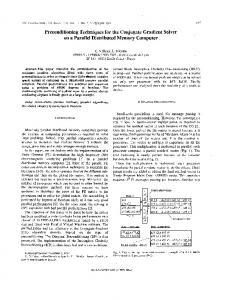
minimum of the absolute value of the function rather than a sign change [53]. The loci of roots of the characteristic function are the dispersion curves for the multilayer plate system. They are usually displayed as phase velocity against frequency but may also be plotted using the wavenumber. A simple method of plotting the curves is to evaluate the function systematically, varying both frequency and velocity over the ranges of interest, and plotting one color for positive results and another for negative results [35]. The resulting plot shows the dispersion curves as the borders between the bands of colors. However this technique is extremely slow and the results are imprecise. A better technique for the calculation of a dispersion curve is to employ some curve following algorithm which starts from a known solution. One possibility for curve following which has been implemented by the author [53] and has been found to be extremely robust, is illustrated in Figs. 4 and 5. Initially, roots are found by varying the phase velocity at fixed frequency or the frequency at fixed velocity (the “sweeps” in Fig. 4). Each of these roots is the starting point for the calculation of a dispersion curve, illustrated in Fig. 5(a). To calculate a dispersion curve, the wavenumber is increased steadily (by fixed increments and a new solution is found at

each step by iteration of the frequency. Clearly the speed of convergence and the stability of the iterations are improved by seeding the root-finding algorithm with a good initial guess of the frequency at each step. In the early stages of tracing a curve (but obviously excluding the first step), the seed is calculated by linear extrapolation from the preceding two solutions. After five steps, a quadratic extrapolation algorithm, shown in Fig. 5(b), is employed in order to obtain a further improvement of the seed. This reduces the time taken to trace a curve but, more importantly, minimizes the risk of following the wrong curve after two dispersion curves cross. Further minimization of this risk is achieved by the use of alternate points in the extrapolation, as illustrated, rather than consecutive points. This is beneficial because it delays the influence of any erroneous points by one step. If the scheme converges on the wrong mode near where two modes cross, then the erroneous point does not affect the extrapolation algorithm immediately, when the curves are still close and the wrong mode could easily be followed, but a step later, when they are diverging again and the risk of finding the wrong curve is much reduced. The scheme works in the wavenumberfrequency space because the dispersion curves are generally closer to straight lines in this form than in others and are therefore easier to follow.

534


(a)

(b) Fig. 5. Generation of dispersion curve. (a) Procedure for generation of curve. (b) Extrapolation scheme.

IV. DEVELOPMENTS OF THE TRANSFER MATRIX METHOD Since the introduction of the Thomson-Haskell matrices, many adaptations and developments have been reported, as summarized in the introduction. The most important developments have been the introduction of wave attenuation and problem, each of which will be the solution of the large discussed in this section. Two other areas of note, which will not be discussed in detail here, are the modeling of fluid layers and the modeling of imperfect boundary conditions between layers. Fluid layers may be introduced specifically into the models [13], [33], [38], [68], [80]–[82] but, as discussed earlier, they may also be approximated successfully using the formulation for solids. Slip boundaries between layers may be modeled by uncoupling the shear stresses between the layer matrices [63], [83], one convenient approach being to include a boundary condition matrix in the assembly of the layers. Boundary condition matrices may also be used to define specific values of stiffness at an interface [52], [78],

[84], [85]. Finally, the field equations for anisotropic properties or cylindrical geometries, which will be discussed in the last section of the paper, alter the sizes of the matrices but involve no changes in principle to the techniques and may readily be introduced. A. Material Damping and Leaky Waves The original Thomson-Haskell matrices describe the fields in the layers in terms of plane waves whose amplitudes are constant in all directions. They are therefore unable to describe the attenuation of reflected or transmitted waves in a damped medium or the decay of a plate wave as it leaks energy into the embedding medium. Both of these possibilities require the introduction of an expression for attenuation in the wave (5) for bulk waves. Material damping may be introduced in a number of ways. A convenient and universally popular [17], [28], [42], [44], [48]–[50], [52], [53], [57], [68]–[70], [82] constitutive model


for small-displacement dynamic behavior in ultrasonic NDE applications is the Kelvin-Voigt viscoelastic description in which a velocity-dependent damping force is added to the equation of motion for an infinitesimal element of the material [77]. Symbolically the model consists of a dashpot representing the damping in parallel with the spring representing the elastic stiffness. It results in a complex wavenumber, the real part of which describes the propagation of the wave and the imaginary part, the attenuation. It thus describes bulk waves whose attenuation per wavelength is constant for all frequencies (attenuation per unit distance therefore increases linearly with frequency). The attenuation of leaky plate waves poses a slightly different problem. Here the field equations for the wave which propagates along the plate must include an attenuation term, even if all of the materials are elastic. This can be achieved by introducing complex wavenumber or complex frequency, either of which will result in an exponential decay factor of (10). In seismological developments, in the invariant, early researchers were uncertain of the best choice, some introducing complex frequency [19]–[21], [23], [25], [27], [86] and others complex wavenumber [24], [29]. Alsop [26] assessed the alternatives and concluded that either approach could be adopted, the more appropriate choice being based on the application in mind. In the following summary, in accordance with more recent publications and with ultrasonics applications [50], [52], [53], [57], [58], [69], [87]–[90], the wavenumber will be assumed to be complex and the frequency real. The imaginary part of the wavenumber vector, which in general is not necessarily parallel to the real part, will therefore account for both material damping and attenuation due to leakage. Referring to (2), the Lamé constants and are replaced by the operators: becomes:

becomes:

(28)

and are the viscoelastic material where the constants is the frequency. The viscoelastic model constants and clearly reduces to the elastic model if the viscoelastic constants are zero. Now the displacement equation of motion (4) can be expressed:

(29) Equation (5) still holds, except that the wavenumber, is now a complex vector so that the functions are of the form: (30) Here the first exponential term, which is wholly imaginary, describes the harmonic propagation of the wave in the direcand the second, real, term describes the tion of the vector exponential decay of the wave with distance in the direction of The decay is therefore described in a spatial the vector

535

manner. It follows that the bulk wave velocities now complex:

and

are

(31) and are related to the bulk wavenumbers by the equations: for longitudinal waves, or for shear waves

(32)

and are parallel, describing a wave whose If decay is strongest in its direction of propagation, then these material constants may also be related to the measurable wave speed and attenuation: or (33)

where is the attenuation in Nepers per wavelength, so that a wave of unit amplitude is reduced to an amplitude of after travelling one wavelength. If the medium is elastic then may exist but it must be normal In most respects the theory may now be developed in an identical fashion as was described for elastic solids, resulting in the same field equations, except that the wavenumber is now a complex vector. This has the particular implication that the coupling of waves at interfaces (Snell’s law) now requires matching of both the propagation characteristics and the attenuations of the bulk waves. The invariant factor of (10) is thus: (34) in which the attenuating exponent describes the decay of all wave components in the direction parallel to the layers, and will therefore describe the decay of leaky or damped plate waves. No changes are required to the Transfer Matrix formulation but there are differences in its solution. For response solutions, the imaginary part of the plate wavenumber must now be specified. A point source on the surface or within a layer may excite waves with all complex values of wavenumber and the modeling of this form of excitation therefore requires a two-dimensional spatial integration. This is a popular requirement in seismological applications and, as discussed in the introduction, may be achieved using a one-dimensional contour integral technique. In ultrasonic applications, the excitation is typically controlled carefully using obliquely aligned transducers. To model such arrangements, it is reasonable to assume that the incident wave has parallel attenuation and propagation directions, thus defining the imaginary part of the plate wavenumber. It follows that the imaginary part of the plate wavenumber vanishes if the coupling medium is elastic.

536

Fig. 6.


Progression of solution for attenuating plate wave.

For modal solutions, the characteristic functions are now complex, depending on frequency, real plate wavenumber and imaginary plate wavenumber. A modal solution therefore yields the rate of decay of a plate wave in addition to its harmonic characteristics. Since the theory for attenuating plate modes is a generalization of the theory for true modes, it is not necessary to classify waves before attempting the modal solution of the equations. The general theory is equally applicable to all classes of plate wave propagation: in cases of attenuating waves the rate of decay is evaluated as part of the solution; in cases of free waves the rate of decay is found during the solution to be zero. The task of finding the complex roots of the characteristic functions for attenuating waves is substantially more difficult than for the real roots and comparatively little has been published. Schwab and Knopoff [28] describe a complex interpolation technique in which the velocity and attenuation are found at a fixed value of frequency. Clayton and Derrick [62] claim to have had success with a complex Regula Falsi method for finding the complex wavenumber at a fixed value of frequency. It resorts to a Monte Carlo technique for restarting when a wild extrapolation occurs. Chimenti et al. [58] employ a complex Newton-Raphson technique, again searching for the complex wavenumber at fixed frequency. Dayal and Kinra [64] use bisection to search for the real part of the wavenumber, and a Secant-Newton technique for the imaginary part. In my own model development [53] I have found that extrapolation schemes, whether real or complex, are prone to instability unless the search is close to a single root

(also observed by Dayal and Kinra [64]) and I prefer simple techniques such as bisection which are robust even if slower to converge. Robustness is a particularly important consideration when undertaking the calculation of dispersion curves when a very large number of solutions is required. My implementation for complex solutions fixes any real variable (frequency, real wavenumber or phase velocity) and solves for the remaining real variable and the attenuation. The solution is found by repeatedly locating the minimum of the absolute value of the function, alternately varying one of the unknowns whilst holding the other constant. The method is illustrated in Fig. 6, the example showing the search for frequency and attenuation at a fixed value of real wavenumber. The example starts with a sweep of frequency at fixed attenuation, from which a minimum of the absolute value . The frequency is then fixed and of the function is found . Alternate the attenuation is varied to find a new minimum searches of frequency and attenuation are continued to find etc.), terminating when a minimum subsequent minima is acceptably close to the origin of the figure. When calculating dispersion curves, a good initial guess of both frequency and attenuation at each step is obtained by extrapolation of the attenuation in the same manner as the frequency (Fig. 5). B. The Problem with Large Values of Frequency-Thickness problem” in the Transfer Matrix technique The “large was first observed by Dunkin [30], since when there have been numerous proposals for its cure, to be discussed shortly. The problem does not relate to the derivation of the technique,


but rather to its numerical implementation, and is manifested by numerical overflow during the solution. The difficulty comes from the requirement for the displacements and stresses at each interface to be expressed in terms of those at the next interface. It can be seen in the assembly of the layer matrix , given explicitly in (19). Consider for example the coefficient . This value displacement at the bottom gives the relationship of the of the layer to that at the top of the layer. The terms and (defined in (14)) are exponential expressions, the exponents being imaginary for homogeneous waves and real for inhomogeneous waves. When the exponents are imaginary the evaluation of is straightforward. However if either exponent is real then the expression contains, in brackets, the sum of a real positive exponential term and a real negative exponential term. There is no problem if the exponents are reasonably close to unity but if the exponents are very large or very small then each of the expressions in brackets consists of the sum of a very large number and a very small number. matrix also consist Similarly the other coefficients of the of sums or differences of large and small numbers. Clearly therefore the matrix becomes ill-conditioned if the exponents are very large and furthermore the problem is not amenable to simple scaling because of the presence of both large and small terms. The condition for the exponent of or to be real is when in (14) is greater than or corresponding to the condition for an inhomogeneous wave. For given material constants and the exponent can also be seen in this equation to be linearly dependent on the product of the frequency and the distance from the top of the layer. Physically now it can be seen that the problem is associated with large exponential decays of inhomogeneous waves through the thickness of the layer. All of the equations describe the relationship of the displacements and stresses at the bottom of the layer to those at the top. The small exponential terms correspond to inhomogeneous waves next to the interface at the top of the layer. For a thick layer or high frequency the depth of penetration of these inhomogeneous waves is small compared to the thickness of the layer. The waves then have little influence on the displacements and stresses at the bottom of the layer and the terms must be small. In the high frequency-thickness limit, these waves at the top of the layer have no influence on the bottom of the layer and the terms must vanish. On the other hand, the large exponential terms correspond to inhomogeneous waves next to the interface at the bottom of the layer. For large values of frequency-thickness, these waves have little influence on the displacements and stresses at the top of the layer. However, because the equations describe the conditions at the bottom of the layer with respect to those at the top, the terms must increase as the frequency-thickness increases. In the high frequency-thickness limit, when the waves at the bottom of the layer have no influence on the top of the layer, the terms must be infinite. I have found in a study utilizing 64 bit precision for real numbers and 128 bit precision for complex numbers that the practical limit for the analysis of the first two modes,

537

and in a titanium plate in vacuum is about 15 MHz-mm (the result would be very similar for aluminum or steel). At high frequencies these two modes consist of inhomogeneous longitudinal and shear waves and are both asymptotic to the Rayleigh wave solution. Look for example at the exponent for shear waves in this case. Assuming a typical value for the is just less than bulk shear velocity and that the product the magnitude of the exponent at 15 MHz-mm is about 30 and so the large and small exponential terms are about and , respectively. The coefficients in the matrix are therefore composed of the sums and differences of numbers which differ by 26 orders of magnitude. C. Reformulations of the Transfer Matrix Method Since the identification of the large problem by Dunkin [30] in 1965, there have been many publications proposing reformulations of the equations to avoid the problem, whilst retaining the concept of a compact transfer matrix. In the same paper, Dunkin himself introduced the “Delta Operator” matrix of all of the technique which uses a subdeterminants of the Transfer Matrix. This separates the exponential terms from the relationships for reflection coefficients which may then be calculated reliably. In its original form however, it does not solve the problem completely, except for surface waves, because transmission coefficients are not separated from the exponentials [56]. Following Dunkin’s proposal, the Delta Operator technique has been adopted and developed by a number of other researchers, leading to various formulations for isotropic solids which have been claimed to be robust [31]–[41], [68]. Some discussion of these developments may be found in References [35], [39], [47] and [56]. More recently, the technique has been developed for the modeling of anisotropic layers, where the transfer matrices are and consequently matrices of subdeterminants must be considered [42], [43]. V. THE GLOBAL MATRIX METHOD In 1964 Knopoff published a fundamentally different matrix formulation for multilayered media [45] which provides an alternative to the Transfer Matrix techniques and may be used problem. It was first implemented by to avoid the large Randall [15] and has subsequently been employed by a number of other researchers [46]–[53], a particularly significant development being the recognition of the importance of the spatial origins of the bulk waves in each layer [48], [49], [52]. The method has the advantages that it is robust and that the same matrix may be used for all categories of solution, whether response or modal, vacuum or solid half-spaces, real or complex plate wavenumber. The disadvantage is that the global matrix may be large and therefore the solution may be relatively slow. The approach with the global matrix method is to assemble directly a single matrix which represents the complete system. equations, where The system matrix consists of is the total number of layers. The equations are based, in sets of four, on satisfying the boundary conditions at each interface. Thus no assumption is made a priori about

538


any interdependence between the sets of equations for each interface. The solution is carried out on the full matrix, addressing all of the equations concurrently. This does not mean that the interfaces are completely independent, because the equations at an interface are influenced by the arrival of waves from the neighboring interfaces. However, as the frequency-thickness product is increased, the influence of an inhomogeneous wave travelling along one interface on the displacements and stresses at the next interface simply reduces. The extent of the influence is determined by the exponential terms in the global matrix. These terms are always decaying functions for inhomogeneous waves, thus in the limit they vanish and an inhomogeneous wave travelling along one interface has no influence on the waves at the next interface (i.e., the layer behaves as a semi-infinite halfspace). The method therefore remains perfectly stable for any frequency-thickness product because it does not rely on the coupling of the inhomogeneous waves from one interface to another. Consider a single interface, for example the second in Fig. 2. Utilizing (15), the displacements and interface stresses at the interface can be expressed as a function of the They amplitudes of the waves at the top of the third layer may also be expressed as a function of the amplitudes of the For continuity of waves at the bottom of the second layer displacements and stresses at the interface, both expressions should give equal results. Therefore

top and bottom of a layer can be expressed, respectively, as: [Dt ] =

k1 k1 g C 0C g iB iBg 2ik1 2 C 02ik1 2 C g [Db ] = k1 g k1 C g 0C iBg iB 2ik1 2 C g 02ik1 2 C

which can be expressed in a single matrix as:

02ik1 2 C iB

C g

0k1 g

02ik1 2 C g iBg

0C g 0k1 g

2ik1 2 C g iBg

0C 0k1

2ik1 2 C

iB

(37) A similar equation to (36) can now be written for the interface and simply added to the global matrix, and similarly for all interfaces, resulting in a matrix of equations and unknowns. In the case of the example in Fig. 2 the matrix equation is:

(38)

where

(35)

C

0k1

the

wave

amplitudes in each layer, have been abbreviated Four of the wave simply to a layer wave vector amplitudes in (38) must now be identified as knowns and their coefficients in the equations moved to the right hand side. For ultrasonics applications it is convenient to choose the incoming waves in the two half-spaces, and as the knowns, giving:

(36)

(39) where the subscripts 2 and 3 refer to layers and and and to the top and bottom of each layer. This equation describes the interaction at interface of the waves in the adjoining and layers Before proceeding, a modification is made to the origins of the bulk waves, which will affect the field (15). Instead of defining the origin for all of the waves in a layer to be the top of the layer, the origin of all waves is defined to be at their entry to the layer. Thus downward travelling waves have their origin at the top of the layer and upward travelling waves have their origin at the bottom of the layer. No change is made for the semi-infinite half-spaces. With this matrices for the modification, and referring to (15), the

where the superscripts + and denote those parts of the matrices or vectors corresponding to and waves, respectively. and each consist of half of the Thus the vectors vector and the matrices and are four-by-two . The partitioning is as follows: partitions of the matrix

(40)


The system matrix on the left hand side of (39) and the sparse matrix on the right hand side are both square and of If the wave amplitudes for the incoming dimension waves are known then the right hand side may be evaluated immediately, resulting in a vector of known coefficients. D. Response Solution Response solutions for the vector of wave amplitudes on the left-hand side of (39) may be obtained readily by inversion (or solution) of the system matrix. This solution is likely to be the most time-consuming part of the analysis. The matrix may be large if many layers are present and the coefficients are complex. Furthermore, the matrix may be close to being singular at times (strictly it actually becomes singular if the wavenumber and frequency correspond precisely to modal solution values). It is therefore worthwhile to employ double precision arithmetic and to implement a solution algorithm which is as efficient and robust as possible. A proven reliable approach [48], [49], [52], [53] is to use Gaussian elimination with partial pivoting, in which the banded nature of the matrix may be exploited to improve efficiency. E. Modal Solution The modal solution for systems in which the half-spaces are not vacuum is straightforward because the system is already described in terms of the wave amplitudes in the half-spaces, in (39). The incoming waves are zero and so the right hand side of the equation must be zero. Thus the system matrix must be singular, so its determinant must be zero. This yields the characteristic function: (41) If the top and bottom half-spaces are vacuum then the and matrices cannot be evaluated. Modification is therefore required to the system matrix to account properly for the absence of waves in vacuum and for zero stresses on the free surfaces. This can be done by reformulating the problem, resulting in a smaller system matrix. The sub-matrices and wave amplitudes associated with the half-spaces are removed from (39) and the remaining top and bottom sub-matrices are partitioned into their stress and displacement rows. The stress partitions are then taken onto the right hand side as knowns, leaving a square system matrix again, and the solution is then possible. However a much simpler alternative [53], which leaves the solution completely general, is to retain the full system matrix and to modify the layer constants for the and vacuum half-spaces in such a way that the matrices can be evaluated, hence solution is possible and the resulting surface stresses are zero. This is achieved by setting the bulk velocities and of the vacuum to arbitrary nonzero values and the density to zero. With these modifications, the matrix assembly and solution is identical to that for the system with nonvacuum half-spaces. The characteristic function of the global matrix method yields a complex value, in general, for all inputs whether for true modes or for attenuating modes. Schwab [46] has shown however that it can be formulated to yield values which lie on

539

either the real or the imaginary axis for true modes. As with the Transfer Matrix method, the solution of the function does not strictly prove the existence of a modal solution, only that the system matrix is singular. In this case there is one other nontrivial circumstance which arises in practice in which the matrix is singular. This is when the plate wavenumber is equal to the wavenumber of either of the bulk waves in any of the internal layers of the system. If this happens then the system matrix has two or more identical columns and is singular. Physically the explanation for this is that the + and waves in this layer both travel parallel to the layer and are therefore indistinguishable in their effect on stresses and displacements at the adjacent interfaces. The importance of a good algorithm for the calculation of the determinant for the modal solution cannot be overstressed. Since the aim is to find zeros of the determinant, the matrix is frequently close to being singular. Furthermore, search algorithms must rely on accurate complex evaluations of the function close to the singularity in order to converge. For the calculation of dispersion curves, the whole process must be repeated very many times without failure. I have found [53] that a perfectly reliable method is to use the reduction part of the Gaussian elimination scheme which was discussed above for the response solution. VI. ANISOTROPIC AND CYLINDRICAL LAYERS The matrix methods which have been summarized in this paper may readily be applied to the modeling of certain other categories of structure which are of interest in nondestructive testing. In particular, the introduction of anisotropic layers enables studies to be made of composite materials, and the introduction of cylindrical layers enables waves in tubular structures to be predicted. The modeling of anisotropic layers is a large topic which has received considerable attention [42]–[44], [65]–[67], [71]–[75] and it will not be examined in any detail here. In principle, the matrix assembly and solution procedures which have been discussed here are applicable to such structures except that the field equations are considerably more complicated. For waves which propagate in one of the principal planes, the field in each layer can still be described in four equations by the superposition of four bulk waves [91]. For general orientations however, it is necessary to extend the matrix to six equations, involving six bulk waves in the layer. There are many publications relating to this theory which may be used for the development of a multilayer model; [44], [66], [67], and [91] include summaries of the developments and explicit expressions for the coefficients of the field matrices. The modeling of waves in a plane through a cylindrical layer may also be achieved using the techniques discussed here, with alternative field equations. The wave equation in cylindrical coordinates cannot be satisfied by exponential functions but may be satisfied by Bessel functions or Hankel functions, representing in the general case three “inward” travelling waves and three “outward” travelling waves. There are thus six equations in the field matrix, describing the three cylindrical displacement coordinates and three of the six

540


stresses. Solutions include motion in the circumferential direction, such as torsional modes, in addition to the motion in the longitudinal-radial plane. Furthermore, the order of the Bessel or Hankel function determines the (integer) circumferential wavenumber. A zero order solution describes waves which are axially symmetric; higher order solutions describe waves whose amplitudes vary sinusoidally around the circumference, the number of sinusoids being equal to the order of the function. Derivations for waves in cylindrical coordinates may be found in [92]–[99]. The derivation presented by Gazis [95], is recommended for its clarity and relative simplicity, although it is limited to elastic waves and true modes. There are also some errors in the equations in [95]: I have observed that the two shear stresses in (17) are incorrect (but these errors do not follow through the later derivations), and there is a term of (19) (the first “ ” minor typing mistake in the should read “ ”). This in fact is the key equation for the implementation of cylindrical field equations. A mistake has also been reported in (27) [100]. VII. CONCLUSIONS Matrix formulations for multilayered media have evolved in the latter half of this century and have featured in a large number of publications, initially for seismological applications and latterly also for ultrasonics. They may be used to develop powerful tools for predicting the response and modal properties of plates. Response models calculate the amplitudes and phases of reflected and transmitted infinite plane waves resulting from a given incident plane wave. Finite fields may then be studied by superposition of the infinite plane wave solutions. Modal models calculate the unforced properties of the system: the velocities and frequencies (dispersion curves) at which plate waves may travel along the plate and their rates of decay. There are currently two quite different approaches to the formulation of the equations and many variants which are in accepted use. The main developments have been reviewed in this paper, concentrating on the aspects which are of particular relevance to ultrasonics. Sufficient details of the derivations of the equations for the “Transfer Matrix” method and the “Global Matrix” method have deliberately been included in the paper in order to benefit researchers who may wish to develop predictive models or to make use of the formulations in analytical investigations. The application and solution of the equations in response and modal models has also been addressed, including discussion based on the author’s own experience of the implementation of both methods. ACKNOWLEDGMENT The author gratefully acknowledges support from the Science and Engineering Research Council in this work; initially under research grant GR/F 65187 and subsequently in supporting me as a Research Fellow. REFERENCES [1] L. Rayleigh, “On waves propagating along the plane surface of an elastic solid,” Proc. London Math. Soc., vol. 17, 1885. [2] R. Stoneley, “Elastic waves at the surface of separation of two solids,” Proc. Roy. Soc., vol. 106, pp. 416–428, 1924.

[3] J. G. Scholte, “The range and existence of Rayleigh and Stoneley waves,” Mon. Not. Roy. Astron. Soc. Geophys. Suppl., vol. 5, pp. 120–126, 1947. [4] W. L. Pilant, “Complex roots of the Stoneley wave equation,” Bull. Seism. Soc. Am., vol. 62, pp. 285–299, 1972. [5] H. Lamb, “On waves in an elastic plate,” Proc. Roy. Soc., vol. 93, PT series A, pp. 114–128, 1917. [6] A. E. H. Love, Some Problems of Geodynamics. London: Cambridge University Press, 1911. [7] W. M. Ewing, W. S. Jardetzky, and F. Press, Elastic Waves in Layered Media. New York: McGraw-Hill, 1957. [8] I. A. Viktorov, Rayleigh and Lamb Waves. New York: Plenum Press, 1970. [9] G. W. Farnell and E. L. Adler, “Elastic wave propagation in thin layers,” in Physical Acoustics, Principles and Methods, W. P. Mason and R. N. Thurston, Eds. New York: Academic Press, 1972, vol. IX, pp. 35–127, 1972. [10] L. M. Brekhovskikh, Waves in Layered Media. New York: Academic Press, 1980. [11] L. M. Brekhovskikh and V. Goncharov, Mechanics of Continua and Wave Dynamics. Berlin: Springer-Verlag, 1985. [12] W. T. Thomson, “Transmission of elastic waves through a stratified solid medium,” J. Appl. Phys., vol. 21, pp. 89–93, 1950. [13] N. A. Haskell, “Dispersion of surface waves on multilayered media,” Bull. Seism. Soc. Am., vol. 43, pp. 17–34, 1953. [14] F. Press, D. Harkrider, and C. A. Seafeldt, “A fast convenient program for computation of surface-wave dispersion curves in multilayered media,” Bull. Seism. Soc. Am., vol. 51, pp. 495–502, 1961. [15] M. J. Randall, “Fast programs for layered half-space problems,” Bull. Seism. Soc. Am., vol. 57, pp. 1299–1316, 1967. [16] T. H. Watson, “A note on fast computation of Rayleigh wave dispersion in the multilayered elastic half-space,” Bull. Seism. Soc. Am., vol. 60, pp. 161–166, 1970. [17] F. A. Schwab and L. Knopoff, “Fast surface wave and free mode computations,” in Methods in Computational Physics, B. A. Bolt, Ed. New York: Academic Press, 1972, vol. IX, pp. 87–180. [18] K. E. Burg, M. Ewing, F. Press, and E. J. Stulken, “A seismic wave guide phenomenon,” Geophysics, vol. 16, pp. 594–612, 1951. [19] J. H. Rosenbaum, “The long-time response of a layered elastic medium to explosive sound,” J. Geophys. Res., vol. 65, pp. 1577–1613, 1960. [20] R. A. Phinney, “Leaking modes in the crustal waveguide. Part 1. The oceanic PL wave,” J. Geophys. Res., vol. 66, pp. 1445–1469, 1961. [21] R. A. Phinney, “Propagation of leaking interface waves,” Bull. Seism. Soc. Am., vol. 51, pp. 527–555, 1961. [22] D. L. Anderson and C. B. Archambeau, “The anelasticity of the earth,” J. Geophys. Res., vol. 69, pp. 2071–2084, 1964. [23] F. Gilbert, “Propagation of transient leaking modes in a stratified elastic wave guide,” Rev. Geophys, vol. 2, pp. 123–153, 1964. [24] S. J. Laster, J. G. Foreman, and A. F. Linville, “Theoretical investigation of modal seismograms for a layer over a half-space,” Geophysics, vol. 30, pp. 571–596, 1965. [25] M. D. Cochran, A. F. Woeber, and J. Cl. De Bremaecker, “Body waves as normal and leaking modes. 3. Pseudo modes and partial derivatives ) sheet,” Rev. Geophys, vol. 8, pp. 321–357, 1970. on the ( [26] L. E. Alsop, “The leaky-mode period equation—a plane-wave approach,” Bull. Seism. Soc. Am., vol. 60, pp. 1989–1998, 1970. [27] A. M. Dainty, “Leaking modes in a crust with a surface layer,” Bull. Seism. Soc. Am., vol. 61, pp. 93–107, 1971. [28] F. A. Schwab and L. Knopoff, “Surface waves on multilayered anelastic media,” Bull. Seism. Soc. Am., vol. 61, pp. 893–912, 1971. [29] T. H. Watson, “A real frequency, complex wave-number analysis of leaking modes,” Bull. Seism. Soc. Am., vol. 62, pp. 369–541, 1972. [30] J. W. Dunkin, “Computation of modal solutions in layered elastic media at high frequencies,” Bull. Seism. Soc. Am., vol. 55, pp. 335–358, 1965. [31] E. N. Thrower, “The computation of dispersion of elastic waves in layered media,” J. Sound Vib., vol. 2, pp. 210–226, 1965. [32] F. Gilbert and G. E. Backus, “Propagator matrices in elastic wave and vibration problems,” Geophysics, vol. 31, pp. 326–332, 1966. [33] R. Kind, “Computation of reflection coefficients for layered media,” J. Geophys., vol. 42, pp. 191–200, 1976. [34] R. Kind, “The reflectivity method for a buried source,” J. Geophys., vol. 44, pp. 603–612, 1978. [35] A. Abo-Zena, “Dispersion function computations for unlimited frequency values,” Geophys. J. R. Astr. Soc., vol. 58, pp. 91–105, 1979. [36] W. Menke, “Comment on ‘Dispersion function computations for unlimited frequency values’ by Anas Abo-Zena,” Geophys. J. R. Astr. Soc., vol. 59, pp. 315–323, 1979. [37] T. Kundu and A. K. Mal, “Elastic waves in a multilayered solid due to a dislocation source,” Wave Motion, vol. 7, pp. 459–471, 1985.

+0


[38] T. Kundu, A. K. Mal, and R. D. Weglein, “Calculation of the acoustic material signature of a layered solid,” J. Acoust. Soc. Am., vol. 77, pp. 353–361, 1985. [39] R. B. Evans, “The decoupling of seismic waves,” Wave Motion, vol. 8, pp. 321–328, 1986. [40] A. K. Mal and T. Kundu, “Reflection of bounded acoustic beams from a layered solid,” in Review of Progress in Quantitative NDE, D. O. Thompson and D. E. Chimenti, Ed. New York: Plenum, 1987, vol. 6, pp. 109–116. [41] D. Lévesque, L. Piché, “A robust transfer matrix formulation for the ultrasonic response of multilayered absorbing media,” J. Acoust. Soc. Am., vol. 92, pp. 452–467, 1992. [42] M. Castaings and B. Hosten, “Delta operator technique to improve the Thomson-Haskell method stability for propagation in multilayered anisotropic absorbing plates,” J. Acoust. Soc. Am., Apr. 1994. [43] M. Castaings and B. Hosten, “Transmission coefficient of multilayered absorbing anisotropic media. A solution to the numerical limitations of the Thomson-Haskell method. Application to composite materials,” in Proc. ULTRASONICS 93, 1993. [44] B. Hosten and M. Castaings, “Transfer matrix of multilayered absorbing and anisotropic media. Measurements and simulations of ultrasonic wave propagation through composite materials,” J. Acoust. Soc. Am., vol. 94, pp. 1488–1495, 1993. [45] L. Knopoff, “A matrix method for elastic wave problems,” Bull. Seism. Soc. Am., vol. 54, pp. 431–438, 1964. [46] F. A. Schwab, “Surface-wave dispersion computations: Knopoff’s method,” Bull. Seism. Soc. Am., vol. 60, pp. 1491–1520, 1970. [47] R. C. Y. Chin, G. W. Hedstrom, and L. Thigpen, “Matrix methods in synthetic seismograms,” Geophys. J. R. Astr. Soc., vol. 77, pp. 483–502, 1984. [48] H. Schmidt and F. B. Jensen, “Efficient numerical solution technique for wave propagation in horizontally stratified environments,” Comp. & Maths. with Appls., vol. 11, pp. 699–715, 1985. , “A full wave solution for propagation in multilayered viscoelas[49] tic media with application to Gaussian beam reflection at fluid-solid interfaces,” J. Acoust. Soc. Am., vol. 77, pp. 813–825, 1985. [50] H. Schmidt and G. Tango, “Efficient global matrix approach to the computation of synthetic seismograms,” Geophys. J. R. Astr. Soc., vol. 84, pp. 331–359, 1986. [51] A. K. Mal, “Guided waves in layered solids with interface zones,” Int. J. Engng. Sci., vol. 26, pp. 873–881, 1988. [52] T. P. Pialucha, “The reflection coefficient from interface layers in NDT of adhesive joints,” Ph.D. dissertation, University of London, 1992. [53] M. J. S. Lowe, “Plate waves for the NDT of diffusion bonded titanium,” Ph.D. dissertation, University of London, 1993. [54] F. R. DiNapoli and R. L. Deavenport, “Theoretical and numerical Green’s function field solution in a plane multilayered medium,” J. Acoust. Soc. Am., vol. 67, pp. 92–105, 1980. [55] G. R. Franssens, “Calculation of the elasto-dynamic Green’s function in layered media by means of a modified propagator matrix method,” Geophys. J. R. Astr. Soc., vol. 75, pp. 669–691, 1983. [56] B. L. N. Kennett, Seismic Wave Propagation in Stratified Media. Cambridge, UK: Cambridge University Press, 1983. [57] P. C. Xu and A. K. Mal, “Calculation of the inplane Green’s function for a layered viscoelastic solid,” Bull. Seism. Soc. Am., vol. 77, pp. 1823–1837, 1987. [58] D. E. Chimenti, A. H. Nayfeh, and D. L. Butler, “Leaky Rayleigh waves on a layered halfspace,” J. Appl. Phys., vol. 53, pp. 170–176, 1982. [59] D. E. Chimenti and A. H. Nayfeh, “Ultrasonic leaky waves in a solid plate separating a fluid and vacuum,” J. Acoust. Soc. Am., vol. 85, pp. 555–560, 1989. [60] T. P. Pialucha and P. Cawley, “The reflection of ultrasound from interface layers in adhesive joints,” in Review of Progress in Quantitative NDE, D. O. Thompson and D. E. Chimenti, Ed. New York: Plenum, 1991, vol. 10, pp. 1303–1309. [61] F. A. Schwab and L. Knopoff, “Surface-wave dispersion computations,” Bull. Seism. Soc. Am., vol. 60, pp. 321–344, 1970. [62] E. Clayton, G. H. Derrick, “A numerical solution of wave equations for real or complex eigenvalues,” Aust. J. Phys., vol. 30, pp. 15–21, 1977. [63] A. Pilarski, “Ultrasonic evaluation of the adhesion degree in layered joints,” Mater. Evaluation, vol. 43, pp. 765–770, 1985. [64] V. Dayal and V. K. Kinra, “Leaky Lamb waves in an anisotropic plate. I: An exact solution and experiments,” J. Acoust. Soc. Am., vol. 85, pp. 2268–2276, 1989. [65] A. H. Nayfeh and D. E. Chimenti, “Propagation of guided waves in fluid-coupled plates of fiber-reinforced composite,” J. Acoust. Soc. Am., vol. 83, pp. 1736–1743, 1988. [66] , “Ultrasonic wave reflection from liquid-coupled orthotropic plates with application to fibrous composites,” J. Appl. Mech., vol. 55,

541

pp. 863–870, 1988. [67] A. H. Nayfeh and D. E. Chimenti, “Elastic wave propagation in fluidloaded multiaxial anisotropic media,” J. Acoust. Soc. Am., vol. 89, pp. 542–549, 1991. [68] P. Cervenka and P. Challande, “A new efficient algorithm to compute the exact reflection and transmission factors for plane waves in layered absorbing media (liquids and solids),” J. Acoust. Soc. Am., vol. 89, pp. 1579–1589, 1991. [69] M. Deschamps and J. Roux, “Some considerations concerning evanescent surface waves,” Ultrason., vol. 29, pp. 283–287, 1991. [70] B. Hosten, “Bulk heterogeneous plane waves propagation through viscoelastic plates and stratified media with large values of frequency domain,” Ultrason., vol. 29, pp. 445–450, 1991. [71] A. H. Nayfeh, “The general problem of elastic wave propagation in multilayered anisotropic media,” J. Acoust. Soc. Am., vol. 89, pp. 1521–1531, 1991. [72] D. Chimenti and A. H. Nayfeh, “Ultrasonic reflection and guided waves in fluid-coupled composite laminates,” J. Nondestructive Evaluation, vol. 9, pp. 51–69, 1990. [73] A. H. Nayfeh and T. Taylor, “Dynamic distribution of displacement and stress consideration in the ultrasonic immersion nondestructive evaluation of multilayered plates,” J. Eng. Mat. and Tech., vol. 112, pp. 260–265, 1990. [74] D. Chimenti and A. H. Nayfeh, “Ultrasonic reflection and guided wave propagation in biaxially laminated composite plates,” J. Acoust. Soc. Am., vol. 87, pp. 1409–1415, 1990. [75] A. H. Nayfeh, “The propagation of horizontally polarized shear waves in multilayered anisotropic media,” J. Acoust. Soc. Am., vol. 86, pp. 2007–2012, 1989. [76] H. Kolsky, Stress Waves in Solids. New York: Dover, 1963. [77] L. E. Malvern, Introduction to the Mechanics of a Continuous Medium. Englewood Cliffs, NJ: Prentice-Hall, 1969. [78] M. Schoenberg, “Elastic wave behavior across linear slip interfaces,” J. Acoust. Soc. Am., vol. 68, pp. 1516–1521, 1980. [79] W. H. Press, B. P. Flannery, S. A. Teukolsky, and W. T. Vetterling, Numerical Recipes. Cambridge, UK: Cambridge University Press, 1986. [80] D. L. Folds and C. D. Loggins, “Transmission and reflection of ultrasonic waves in layered media,” J. Acoust. Soc. Am., vol. 62, pp. 1102–1109, 1977. [81] D. B. Bogy and S. M. Gracewski, “Reflection coefficient for plane waves in a fluid incident on a layered elastic half-space,” J. Appl. Mech., vol. 50, pp. 405–414, 1983. [82] D. F. McCammon and S. T. McDaniel, “The influence of the physical properties of ice on reflectivity,” J. Acoust. Soc. Am., vol. 77, pp. 499–507, 1985. [83] A. H. Nayfeh and T. W. Taylor, “Surface wave characteristics of fluid-loaded multilayered media,” J. Acoust. Soc. Am., vol. 84, pp. 2187–2191, 1988. [84] S. I. Rokhlin and Y. J. Wang, “Analysis of boundary conditions for elastic wave interaction with an interface between two solids,” J. Acoust. Soc. Am., vol. 89, pp. 503–515, 1991. [85] T. Pialucha, M. J. S. Lowe, and P. Cawley, “Validity of different models of interfaces in adhesion and diffusion bonded joints,” in Review of Progress in Quantitative NDE, D. O. Thompson and D. E. Chimenti, Ed. New York: Plenum, 1993, vol. 12. [86] F. Abramovici, “Diagnostic diagrams and transfer functions for oceanic wave-guides,” Bull. Seism. Soc. Am., vol. 58, pp. 427–456, 1968. [87] A. H. Nayfeh, D. E. Chimenti, L. Adler, and R. L. Crane, “Ultrasonic leaky waves in the presence of a thin layer,” J. Appl. Phys., vol. 52, pp. 4985–4994, 1981. [88] P. B. Nagy and L. Adler, “Nondestructive evaluation of adhesive joints by guided waves,” J. Appl. Phys., vol. 66, pp. 4658–4663, 1989. [89] D. E. Chimenti and S. I. Rokhlin, “Relationship between leaky Lamb modes and reflection coefficient zeroes for a fluid-coupled elastic layer,” J. Acoust. Soc. Am., vol. 88, pp. 1603–1611, 1990. [90] P. B. Nagy, D. V. Rypien, and L. Adler, “Dispersive properties of leaky interface waves in adhesive layers,” Review of Progress in Quantitative NDE, D. O. Thompson and D. E. Chimenti, Ed. New York: Plenum, vol. 9, pp. 1247–1255, 1990. [91] B. Hosten and M. Castaings, “Validation at lower frequencies of the effective elastic constants measurements for orthotropic composite materials,” Review of Progress in Quantitative NDE, D. O. Thompson and D. E. Chimenti, Ed. New York, Plenum, vol. 12, pp. 1193–1199, 1993. [92] G. E. Hudson, “Dispersion of elastic waves in solid circular cylinders,” Phys. Rev., vol. 63, 1943. [93] M. C. Junger and F. J. Rosato, “The propagation of elastic waves in thinwalled cylindrical shells,” J. Acoust. Soc. Am., vol. 26, pp. 709–713, 1954.

542


[94] I. Mirsky and G. Herrmann, “Nonaxially symmetric motions of cylindrical shells,” J. Acoust. Soc. Am., vol. 29, pp. 1116–1123, 1957. [95] D. C. Gazis, “Three-dimensional investigation of the propagation of waves in hollow circular cylinders. I. Analytical foundation,” J. Acoust. Soc. Am., vol. 31, pp. 568–578, 1959. [96] A. H. Meitzler, “Mode coupling occurring in the propagation of elastic pulses in wires,” J. Acoust. Soc. Am., vol. 33, pp. 435–445, 1961. [97] I. A. Viktorov and O. M. Zubova, “Normal plate modes in a solid cylindrical layer,” Soviet Physics—Acoustics, vol. 9, pp. 15–17, 1963. [98] J. Zemanek, “An experimental and theoretical investigation of elastic wave propagation in a cylinder,” J. Acoust. Soc. Am., vol. 51, pp. 265–283, 1972. [99] C. Randall and F. E. Stanke, “Mathematical model for internal ultrasonic inspection of cylindrically layered structures,” J. Acoust. Soc. Am., vol. 83, pp. 1295–1305, 1988. [100] I. Mirsky and G. Herrmann, “Nonaxially symmetric motions of cylindrical shells,” J. Acoust. Soc. Am., vol. 31, p. 250, 1959.

Michael J. S. Lowe received the B.Sc. degree in civil engineering from the University of Edinburgh in 1979, and the M.Sc. and Ph.D. degrees in mechanical engineering from Imperial College, University of London, in 1987 and 1993, respectively. From 1979 to 1989 he worked in engineering consultancy, specializing in the application and development of numerical methods for the solution of problems in solid mechanics. His principal clients were the nuclear power and offshore oil industries. Since 1989 he has been working in the NDE research group in the Department of Mechanical Engineering at Imperial College, University of London, where he is currently a SERC Research Fellow. His research work has addressed the detection of weak interfaces in diffusion and adhesive bounded joints and the long-range inspection of structures using plate waves.

Matrix Techniques for Modeling Ultrasonic Waves in ... - IEEE Xplore

Matrix Techniques for Modeling Ultrasonic Waves in ... - IEEE Xplore

Suggest Documents

Matrix Techniques for Modeling Ultrasonic Waves in ... - IEEE Xplore

Ultrasonic Field Modeling: A Comparison of Analytical ... - IEEE Xplore

Modeling of ultrasonic fields and their interaction with ... - IEEE Xplore

Modeling and Optimization Techniques for Yield-Aware ... - IEEE Xplore

Modeling and Optimization Techniques for Yield-Aware ... - IEEE Xplore

Flat Optics for Surface Waves - IEEE Xplore

Flat Optics for Surface Waves - IEEE Xplore

Phononic Plate Waves - IEEE Xplore

Growing Evanescent Waves in Continuous ... - IEEE Xplore

Electromagnetic Waves in Perfect Electromagnetic ... - IEEE Xplore

Ultrasonic Scanner for In Vivo Measurement of ... - IEEE Xplore

Compensating for Tissue Changes in an Ultrasonic ... - IEEE Xplore

Spin Waves and Electromagnetic Waves in Photonic ... - IEEE Xplore

Finite Element Modeling of Ultrasonic Waves in Viscoelastic Media

Regularization in Matrix Relevance Learning - IEEE Xplore

Ultrasonic Waves in Mining Application

Preconditioning Techniques For The Conjugate ... - IEEE Xplore

Development of an Ultrasonic Clutch - IEEE Xplore

A Micromachined Piezoelectric Ultrasonic Transducer ... - IEEE Xplore

Novel Preprocessing Techniques for Accurate ... - IEEE Xplore

Mathematical Decomposition Techniques for Distributed ... - IEEE Xplore

Contingency Filtering Techniques for Preventive ... - IEEE Xplore

capacitive micromachined ultrasonic transducers - IEEE Xplore

PSpice Simulation of Ultrasonic Systems - IEEE Xplore