PREPRINT Published as: Kiprakis, A.E.; Wallace, A.R., "Maximising energy capture from distributed generators in weak networks," in Generation, Transmission and Distribution, IEE Proceedings- , vol.151, no.5, pp.611-618, 13 Sept. 2004, DOI: 10.1049/ip-gtd:20040697 Maximising Energy Capture from Distributed Generators in Weak Networks Aristides E Kiprakis and A Robin Wallace∗ Abstract This paper discusses the implications of the increasing capacity of synchronous generators at the remote ends of rural distribution networks where the line resistances are high and the X/R ratios are low. Local voltage variation is specifically examined and two methods of compensation are proposed. The first of them is a deterministic system that uses a set of rules to intelligently switch between voltage and power factor control modes, while the second is based on a Fuzzy Inference System that adjusts the reference setting of the Automatic Power Factor Controller in response to the terminal voltage. Extensive simulations have verified that the proposed approaches may increase the export of real power while maintaining voltage within the statutory limits.
1. Introduction Increased environmental awareness has generated a number of directives such as the EU Renewables Directive and the UK Renewables Obligation, in order to motivate development of Renewable Energy (RE) resources including Mini-Hydro and Combined Heat and Power (CHP) plants. The Renewables Obligation sets a target that by 2010 10% of total electricity supplied should be from RE plant. In absolute terms this implies connection of around 2000 MW of new DG plant every year [1]. A great amount of this new generation (especially RE) is typically found in remote rural areas where the loads are low, the Distribution Network (DN) is medium or even low voltage and designed for a unidirectional, downstream flow of energy [2]. The steady-state, slow and transient variations of voltage levels related to the connection of a DG can lead to undesired operation of voltage control equipment on transformers at the primary substations of the network. A net reversal or increase of power flow in line due to the presence or the loss respectively of a DG, can cause unacceptable voltage variations and the Distribution Network Operator (DNO) will then require that the DG be disconnected [3]. Operation of DGs under constant voltage or constant power factor (PF) mode may require network reinforcement in order to reduce voltage variation and the cost of this work may be attributed to the connection costs of the DG. This may make potential schemes less attractive or even impossible to implement [2, 3]. Recent developments involving mixed voltage/PF control have shown that by intelligently controlling synchronous generators (SGs) voltage variations can be mitigated and reinforcement may be avoided ∗Both
authors are with the Institute for Energy Systems, University of Edinburgh, King’s Buildings, Mayfield Road, Edinburgh,
EH9 3JL, UK. Emails:
[email protected],
[email protected]
1
-2-
[3]. Utilisation of a Fuzzy Logic (FL) Controller to control the DG may also prove to be a means of reducing or deferring network reinforcement.
2. Impact of Increased Dispersed Generation in Weak Rural Networks The distribution network has been significantly extended during the last 50 years, but its structure and operation has remained largely unchanged [4]. Energy is transfered from the bulk supply points (connection to the transmission grid) towards the far ends of the DN using overhead lines. Moving away from the primary substation the loads become smaller and this has allowed the DNOs to use conductors of decreasing cross-sectional area in order to reduce network development costs. However, this means that the network resistance R per kilometre increases. This has serious implications for the development of DG projects located close to the remote ends of the DN as the increased resistance will exaggerate the variation of voltage due to generated power export.
Figure 1: Radially tapered network
In an 11 kV radially-tapered network such as the one shown in Figure 1, the bus voltages in per unit are derived from the equation:
Vn+1 = V1 −
n X (Rk + jXk )(Pk+1 − jQk+1 ) k=1
Vk+1
pu
(1)
The statutory limits on the 11 kV network are typically ±6%. The voltage profile of the network of Figure 1 when the generator on bus 4 is disconected is shown in Figure 2.(a). It is obvious that although the
-3-
loads are equal, the voltage gradient increases towards the end of the line due to the higher line impedance.
5−bus system − DG disconnected
5−bus system − DG connected 1.15 P = 0.5 pu P = 1.0 pu
1.03
1.12 Bus voltage (pu)
Bus voltage (pu)
1.02
1.09
1.01
1.03
0.99 0.98
Voltage limit = 1.06 pu
1.06
1
1
2
3 Bus number
(a) DG disconnected
4
5
1
1
2
3 Bus number
4
5
(b) DG connected
Figure 2: Voltage profile of the radially tapered network Connection of the 20 MW generator operating at 0.9 lagging constant power factor on bus 4 would alter the voltage profile of the line as shown in Figure 2.(b). The voltages on bus 4, as well as the neighbouring buses 3 and 5, are outside the allowable range. To remain connected, the generator should decrease its output to 0.5 pu in order to bring voltage back within the statutory limits. Other than network reinforcement, alternative measures to accommodate the added DG capacity could include [5]: Operating the DG at leading power factor. Voltage rise may be mitigated, to some extent, by operating at or below unity power factor, but the need to import excessive reactive power would have to be discussed with the DNO. Lowering the primary substation voltage. The DNO can reduce the set-point voltage at the primary substation reducing all voltages further down the feeder. However, due to the variable nature of RE sources and non-dispatched nature of the DGs, the possibility of loss of generator cannot be neglected. Should this happen, the voltages would be further reduced, perhaps below the statutory limits. Operating the DG in constant voltage mode. Disallowed by most DNOs until recently, operating in voltage control mode may help to maintain voltages within acceptable levels, but the voltage dictated by the DG may lead to conflicts of control with the DNO’s transformer auto tap-changer settings.
-4-
3. Automatic Voltage / Power Factor Controller The operating constraints that the DNO imposes on the DG (i.e. ranges of permissible voltage and power factor values) are shown in the voltage vector diagram of Figure 3. In this diagram Vmin and Vmax are the minimum and maximum acceptable voltages and P Fmin and P Fmax are the lines of constant minimum and maximum power factor, respectively.
Figure 3: Voltage vector diagram for the two-bus system of Figure 5 The allowable area of operation is the shadowed region between these boundaries. The block diagram of a possible system that restricts operation of the synchronous generator within the shadowed area is shown in Figure 4. Details of excitation systems and synchronous machine modelling have been presented extensively in [6, 7, 8] and are not going to be discussed here.
Figure 4: AVPFC controlled synchronous generator block diagram After synchronisation, the DG could be brought towards capacity in constant power factor mode (travel-
-5-
ling out on its constant power factor line) until the busbar voltage exceeded a pre-defined threshold voltage within the statutory limits. At that point APFC could be replaced with AVC to vary excitation and move the operating point around the constant voltage circle within the busbar overvoltage limit. Increased local load and reduction in terminal voltage could take the system back into APFC by sensing the increased demand for reactive power and therefore the reduction of power factor. Variations in network impedance would have a similar effect. This system would also enable voltage support at times of heavy local demand. On reaching a voltage just above the undervoltage limit the excitation system would be transferred to AVC to maintain local voltage. Excitation under- and over-voltage and over-current protection should protect the DG excitation and control system against prolonged forcing. When AVC is active the APFC module is disengaged, otherwise the non-zero power factor error signal would saturate the integrator of the internal PID compensator.
3.1. Determination of AVPFC mode selection rule set The control block in Figure 4 is responsible for the control mode decision making. The system will attempt to regulate the DG operation around one of three possible setpoints: the power factor setting P Fref , and the high or low voltage setting Vh and Vl , respectively. Table 1 shows the heuristics of the control algorithm i.e., the reference value which is applied to the controller for every combination of voltage and power factor conditions. In order to prevent hunting, a deadband exists around the decision thresholds. Voltage deadband is annotated as VD and power factor deadband is P FD .
P F ≤ P FB P FB < P F < P FT P FT ≤ P F
V2 ≤ VB VB Vl Vl P Fref
< V 2 < V T VT ≤ V2 P Fref P Fref P Fref Vh P Fref Vh
Table 1: AVPFC mode selection rules set
where:
VB = Vl − VD , VT = Vh + VD , P FB = P Fref − P FD ,
and
P FT = P Fref + P FD . When voltage is within the statutory limits the DG is in APFC mode and tries to set the power factor at
P Fref . When a voltage higher than VT is detected and at the same time the power factor is equal or higher than P FB , the controller will switch to AVC and will try to adjust V2 to Vh . However, if the power factor is lower than P FB the controller will operate in APFC, because its attempt to raise the power factor will result in lowering the terminal voltage (and thus the exported reactive power).This way it is ensured that the
-6-
system will never lock into one of its states. The inverse procedure is followed when the terminal voltage is lower than VB . 3.2. Performance of the DG under AVPFC control In order to test model validity, the process of generator load-up was simulated under AVPFC control and the results compared with those under AVC and APFC modes. The radial test network in Figure 5 was used with its characteristics shown in Table 2. The results of the DG loading-up, post-synchronisation, are shown in Figure 6.
Figure 5: Basic 2 bus system
Network Data Machine size: 10 MW Load size PL , QL : 4 MW, 3 MVAr Line resistance R: 0.124 pu Line reactance X: 0.099 pu Network Voltage V1 : 1.0 pu Base Voltage Vbase : 11 kV Base Power Sbase : 10 MVA AVPFC Data Vh : 1.03 pu Vl : 0.97 pu VB : 0.0025 pu P Fref : 0.9 lagging P FB : 0.0025 APFC Data P Fref : 0.9 lagging AVC Data Vref : 1.03 pu Table 2: Test system data In this (hypothetical) case, local power demand is sufficiently high to result in the voltage at bus 2 (V2 ) lying below the 0.94 pu limit. Normally, however, DNOs would ensure that voltage remained within statutory limits prior to connection. In the initial stages of load-up (t ≤ 45 sec), local power demand exceeds DG output and in the case of the APFC-controlled DG, is sufficiently high to result in voltage V2 being below 0.94 pu (a hypothetical situation as in general DNOs would ensure voltage remained within statutory limits prior to connection). During the same period a fixed-voltage, AVC-controlled generator would try to hold voltage at the 1.03
-7-
pu reference voltage leading to significant reactive power generation and a fall in the power factor wherein the DG excitation protection devices would shut the plant down. The AVPFC controller responded by fixing the terminal voltage at 0.97 pu. The low power factor would cause the protection devices to shut the generator down, albeit for a significantly shorter time than in the AVC case. Between t = 45 sec and t = 125 sec the AVPFC operated the generator in constant power factor mode as this would not result in voltage excursions outside the preset thresholds. For that period the response of the controller was identical to the response of APFC.
Exported real power Pexp (pu)
0.4 0 −0.4
Qexp (pu)
Exported reactive power 0.5 0 −0.5 SG power factor PF
0.8 0.4
APFC AVPFC AVC
0
V2 (pu)
Terminal voltage High voltage limit = 1.06 pu
1.03 0.97
Low voltage limit = 0.94 pu 0
50
100
150
time (sec)
Figure 6: DG loading-up under AVC, APFC and AVPFC control At t = 125 sec, the voltage of the APFC and AVPFC controlled generators reached 1.03 pu. Under AVPFC there was a switch to voltage control to maintain voltage and from this point on its response is identical to that with AVC. The voltage under APFC continued to rise towards and through 1.06 pu - overvoltage protection would trip the DG at that point.
-8-
4. Fuzzy Logic Power Factor Controller (FLPFC) Artificial Intelligence has been applied successfully to solve many power system problems. Being highly nonlinear, power systems are very difficult to control with conventional methods and linearisation techniques very often fail to produce models that resemble the actual characteristics of the system. The resulting ambiguities impose constraints on power system controller design. In addition to this, the stochastic variation of load, generation and topology of a power system exaggerate uncertainty and imprecision [9]. The use of a fuzzy inference-based approach can overcome these difficulties.
4.1. Formulation of the problem A conventional automatic power factor controller has a flat power factor characteristic over the permissible range of voltage. A human operator (or, indeed, an intelligent controller) of the DG plant may be able to respond to voltage variation by altering the power factor setpoint in a way that the change in generated (or absorbed) reactive power regulated the terminal voltage. The desired voltage - tan(φ) relationship is shown in Figure 7.
Figure 7: Desired relationship between voltage and tan(φ) The DG should operate with constant tan(φ) = tan(φnom ) (i.e. constant power factor) in the band [VTl , VTh ] in the middle of the permissible voltage range [VTmin , VTmax ]. When voltage falls, tan(φ) should rise to tan(φmax ), so that the extra reactive power generation restores voltage. Conversely, raised voltage would require tan(φ) to drop (even below zero for a leading power factor) to tan(φmin ) to compensate for the voltage increase. It is possible to achieve such operation by adjusting the power factor reference according to a signal generated from measurements of the terminal voltage via a Look-Up Table (LUT). The block diagram of a DG controlled in this manner is shown in Figure 8.
-9-
Figure 8: Block diagram of a DG with a Fuzzy Logic Power Factor Controller The LUT behaves as a standard numerical input - numerical output, nonlinear element of a closed-loop control system [10] but even though the controller is a number - to - number mapping, as discussed in the next section, it is designed with a procedure that relies on Fuzzy Inference Systems (FIS) theory. It should be stressed that this nonlinear mapping is not unique and is heavily affected by the conversion procedure of the fuzzy control sets [10]. Furthermore, extrapolation capabilities should be given to the LUT to enable it to produce an output even when the input is outside the design limits.
4.2. Design of the Fuzzy Logic Power Factor Controller From the two available types of Fuzzy Logic (FL) controllers (Madamani-type and Sugeno-type), the one proposed by Sugeno [11] has superior control performance [12]. Once the desired controller response has been identified, there is a number of steps that have to be followed, namely the design of the input stage (fuzzification), determination of the fuzzy rules, and design of the output stage (defuzzification).
4.2.1. Design of the input stage Since this is a Single Input - Single Output (SISO) controller, the input fuzzy set consists only of the measured terminal voltage VT , varying over the range [VTmin , VTmax ]. Three linguistic labels define voltage; LOW (L), NORMAL (N) and HIGH (H) and correspond to to the three areas of the curve in Figure 7. The (Gaussian) input membership functions are shown in Figure 9 and are described by Equations 2 - 4: LOW: AL (VT ) ∀VT ∈ [VTmin , VTmax ]
" µ ¶2 # VT − VTmin = exp − VTl − VTmin
(2)
- 10 -
· ³ ´2 ¸ VT −VT1 exp − V −V ,VTmin ≤ VT < VT1 Tl T1
NORMAL: AN (VT ) =
1
,V
≤V
≤V
T1 T T2 · ³ ´2 ¸ V −V exp − V T −VT2 ,VT2 < VT ≤ VTmax T T h
HIGH: AH (VT )
(3)
2
" µ ¶2 # VT − VTmax = exp − VTh − VTmax
(4)
∀VT ∈ [VTmin , VTmax ]
Input membership functions
1 0.9 0.8
membership µ
0.7 0.6 LOW NORMAL HIGH
0.5 0.4 0.3 0.2 0.1 0
0.95
1 1.05 Terminal voltage Vt (pu)
Figure 9: Input membership functions
4.2.2. Determination of the fuzzy rules A typical rule in a Sugeno - type fuzzy model has the form [11]: IF Input = xi , THEN Output is yi = ai xi + bi , where i is the index of the fuzzy rule. For a zero - order Sugeno model, the output level y is a constant (a = 0). Therefore the fuzzy rule set becomes: 1. IF (VT = LOW ) THEN (u1 = P Fmin ) 2. IF (VT = N ORM AL) THEN (u2 = P Fnom ) 3. IF (VT = HIGH) THEN (u3 = P Fmax ) where u1 , u2 , u3 are the outputs of the respective fuzzy rules.
- 11 -
4.2.3. Design of the output stage The output level ui of each fuzzy rule is weighted by the level of activation µi of the rule (see Figure 9). The final output of the system is the weighted average of all rule outputs, computed as P3 P Fref = Pi=1 3
µi ui
i=1
(5)
µi
4.3. Performance of the DG under FLPFC control To quantify the benefit of using the FLPFC, a simulation on a system identical to the one in Section 3.2 was performed, this time with the DG under FLPFC control. The details of the FLPFC are shown in Table 3.
VTmax : VTmin : VTh : VTl : VT 2 : VT 1 : tan(φmax ) : tan(φnom ) : tan(φmin ) :
FLPFC Data 1.05 pu 0.95 pu 1.04 pu 0.96 pu 1.03 pu 0.97 pu 0.750 (P Fmin = 0.8 lagging) 0.484 (P Fnom = 0.9 lagging) −0.329 (P Fmax = 0.95 leading)
Table 3: Fuzzy Logic Power Factor Controller data Application of the data of Table 3 on the FLPFC produced a LUT with the response shown in Figure 10.
FLPFC LUT response 0.8 PFmin = 0.8 lagging 0.6
Output
0.4
PFnom = 0.9 lagging
0.2
0
−0.2 PFmax = 0.95 leading −0.4
0.95
1
Input Figure 10: LUT response
1.05
- 12 -
The results of the simulation are shown in Figure 11. The response of the AVC and APFC controlled DGs are shown for comparison. Early in the loading process the FLPFC slightly pushes voltage up in the operational envelope. This is because the FLPFC allows the SG to operate at 0.8 power factor exporting extra reactive power.
Pexp (pu)
Exported real power 0.4 0 −0.4
Qexp (pu)
Exported reactive power 0.5 0
SG power factor
PF
0.8
APFC AVC FLPFC
0.4 0
V2 (pu)
Terminal voltage Higher voltage limit = 1.06 pu
1.03 0.97
Lower voltage limit = 0.94 pu 0
50
100
150
time (sec)
Figure 11: DG loading-up under AVC, APFC and FLPFC control
In the middle section of the loading process and while voltage lies between 0.97 pu and 1.03 pu the system operates at constant 0.9 PF, almost identical to the APFC and AVPFC cases. When voltage rises above 1.03 pu, the FLPFC starts decreasing the power factor setpoint - increasing tan(φnom ) - and by constraining Qexp , the terminal voltage is held within acceptable levels. It should be noted that the the FLPFC (as well as the AVPFC) will maintain the voltage within the permissible range only as long as the reactive power limits have not been met. These three tests showed that for the same network conditions, utilisation of either AVPFC or FLPFC would be beneficial as their operational margins are wider compared to the traditional fixed power factor operation of a synchronous generator.
- 13 -
5. Simulation of operation of APFC, AVPFC and FLPFC controlled DG under real-time varying load conditions To test the response of the DG to voltage variations brought about by changes in local load under the control of APFC, AVPFC and FLPFC, a time-varying load was connected to the DG busbar of the 2-bus network in Figure 5 to simulate the time variation of actual aggregated load at a DN substation. The network characteristics are given in Table 4.
Network Data Machine size: 4.0 MW Min. Load PL , QL : 1.11 MW, 0.538 MVAr Max. Load PL , QL : 6.411 MW, 3.105 MVAr Load power factor PF: 0.9 Line resistance R: 0.1901 pu Line reactance X: 0.1521 pu Network Voltage: 1.0 pu Base Voltage Vbase : 11 kV Base Power Sbase : 10 MVA Table 4: Test system data Figure 12 shows the actual demand profile that was applied at constant 0.9 power factor over a 24-hour period. It resembles an aggregated 80% domestic - 20% industrial load.
24hour load profile (0.9 PF) 7 6
PL (MW)
5 4 3 2 1
0
3
6
9 12 15 18 21 24 time (hours)
Figure 12: 24-hour, 80 % domestic 20% industrial load profile
The simulation was performed three times; at first with the APFC, then with the AVPFC and lastly with the FLPFC. The settings of APFC and FLPFC were the same as the ones used for the generator loading
- 14 tests (see Tables 2 and 3). Setpoints Vh and Vl of the AVPFC have been changed to 1.04 p.u and 0.96 p.u. respectively in order to match to the FLPFC ones. Additionally, the power factor of the generator has been constrained between 0.8 lagging and 0.95 leading to resemble real-life operation in a DN, as a DNO would generally not allow a generator to operate with an unconstrained PF. The response of a typical APFC generator setup is shown in Figure 13.
Pexp (MW)
Exported MW 3 0 −3
Qexp (MVAr)
Exported MVAr 1.5 0
−1.5 Generator’s PF
PF
0.91 0.9
0.89 Bus voltage
1.0
U/V
V2 (pu)
1.06 OFF
0.94 0
3
6
9 12 15 time (hours)
18
21
24
Figure 13: Response of APFC to a varying load
The power factor of the generator remains constant throughout the whole period. However, for the period between 0:45-06:15 hours the generator would be disconnected as the large (constant) amount of generated power in combination with the low local demand would cause excessive power export and thus voltage violation. Additionally, during the 17:15-18:45 hours high local demand period, the bus voltage would be below the 0.94 p.u. statutory limit. Figure 14.(a) shows the response of an AVPFC controlled SG under the same circumstances. Compared to the APFC controlled SG response, it is apparent that for the periods while the bus voltage would be in the 0.97 pu - 1.03 pu region, the operation of the two systems is identical. However, during the periods of low (00:30-07:00 hours) and high (17:15-19:30 hours) demand, the AVPFC switches to constant voltage mode and holds voltage at 1.04 pu and 0.96 pu, respectively. This results in a longer period of operation,
- 15 -
more energy shipped to the network and therefore increased revenue for the developer. It should be noted that for a short period just before 18:00 hours the voltage falls below the 0.95 p.u. setpoint, because the power factor limit has been met and the generator cannot support voltage any further.
Exported MW Pexp (MW)
Pexp (MW)
Exported MW 3 0 −3
3 0 −3
1 0 −1 Generator’s PF
1 0 −1 Generator’s PF
1 PF
1 PF
Exported MVAr Qexp (MVAr)
Qexp (MVAr)
Exported MVAr
0.9 0.8
0.9 0.8
Bus voltage
Bus voltage 1.06 V2 (pu)
V2 (pu)
1.06 1.0
0.94
1.0
0.94 0
3
6
9 12 15 time (hours)
(a) AVPFC response
18
21
24
0
3
6
9 12 15 time (hours)
18
21
24
(b) FLPFC response
Figure 14: AVPFC (a) and FLPFC (b) response to 24-hour varying load Figure 14.(b) presents the results of simulations under FLPFC control. It is clear that neither voltage nor power factor exceed their operational range and therefore the generator will remain connected for the whole period of simulation, resulting in an extra 22 MW-hours exported energy compared to APFC operation. For a 4 MW machine, this represents considerable increase in output with consequent financial benefits, particularly if the DG qualifies for Renewable Obligation Credits.
6. Discussion There is a need for DGs to be able to operate flexibly within a voltage envelope to maximise dispatch of active power and to support the voltage in cases of high demand. Some DNOs are now prepared to consider and integrate DGs that can operate to provide voltage control services. Network reinforcement costs may be deferred and loss of generation due to under- or over-voltage shutdown may be reduced. Network, generator
- 16 -
and excitation system protection settings and timings will require to be applied carefully, within statutory and manufacturers limits to ensure that the DG plant operates within accepted network voltages and machine ratings. While voltage and power factor control techniques are well established, their combination has never been coordinated, actively, to sustain production of real power in a weak network. Active transfer between voltage and power factor control modes and fuzzy logic DG control have been shown to allow extended operation when network or local demand conditions would otherwise cause excessive voltage variation and plant shutdown. The presented simulations show that in both AVPFC and FLPFC cases the 24-hour uninterrupted operation would cause an extra 22 MW-hours exported from a 4 MW generator, compared to the traditional APFC scheme. Possible solutions to maintain constant operation of an APFC controlled generator could be network reinforcement, or utilisation of an On-Line Tap Changing (OLTC) transformer but this would increase the capital and/or maintenance costs and could make a potential project infeasible. Utilisation of these new control algorithms could make potential DG projects more attractive by allowing the generator capacity to increase further before it causes a voltage violation. Overall generator and prime mover control is frequently incorporated in Programmable Logic Controllers (PLCs) and this may make the implementation of the presented algorithms easier due to their rule-based nature.
7. Conclusions In this paper the impact of an increased generation capacity in the distribution network was discussed. This made apparent the need for an intelligent control strategy for the Distributed Generation and two candidate solutions were proposed: a hybrid voltage / power factor controller and a fuzzy logic power factor controller. Both algorithms allowed extension of generator operating period in a weak network and therefore an increase of the revenue from energy export. This was illustrated by computer simulations of a DG in a rural network using a realistic local load pattern. However, the developer should discuss with the DNO in beforehand about the adoption of the AVPFC scheme because the generator’s settings may conflict with those of the network equipment when in constant voltage mode. On the other hand, adoption of the Fuzzy Controller scheme can be straightforward, provided that the controller is set to operate within the voltage and power factor limits set by the machine specifications and the DNO.
Acknowledgements The authors acknowledge with gratitude support provided by EPSRC under grant RNET/GR/N04744, and Scottish Power plc. Dr Gareth Harisson’s input to this paper through discussions and comments is also greatly appreciated.
- 17 -
References [1] Wallace A. R.,“Protection of Embedded Generation Schemes”, IEE Colloquium on Protection and Connection of Renewable Energy Systems, pp. 1/1-1/5, 9th November 1999. [2] Harrison G. P., Kiprakis A. E. and Wallace A. R., “Network Integration of Mini-Hydro Generation in Liberalised Markets”, International Water Power and Dam Construction, vol. 54, no. 11, November 2002. [3] Wallace A. R. and Kiprakis A. E., “Reduction of Voltage Violations from Embedded Generators Connected to the Distribution Network by Intelligent Reactive Power Control”, Proc. 5th Int. Conf. on Power System Management and Control, pp. 210-215, 2001. [4] Scottish Excecutive, “Impact of Renewable Generation on the Electrical Transmission Network in Scotland”, October 2001. [5] Masters C. L., “Voltage Rise: the Big Issue When Connecting Embedded Generation to Long 11kV Overhead Lines”, IEE Power Engineering Journal, vol. 16, no. 1, pp. 5-12, February 2001. [6] “Recommended Practice for Excitation System Models for Power System Stability Studies”, IEEE Standard 421.5-1992, August 1992. [7] Grainger J. J. and Stevenson W. D. Jr., “Power System Analysis”, sec. 3.5, McGraw-Hill, 1994. [8] Saadat H., “Power System Analysis”, WCB/McGraw-Hill, 1999. [9] Song Y.-H. and Johns A. T., “Applications of Fuzzy Logic in Power Systems, Part 1”, IEE Power Engineering Journal, vol. 11, no. 5, pp. 219-222, October 1997. [10] Pedrycz W., “Fuzzy Control And Fuzzy Systems, 2nd ed.” sec. 4.5, Research Studies Press, 1993. [11] Takagi T. and Sugeno M., “Fuzzy Identification of Systems and its Application to Modelling and Control”, IEEE Trans. Syst., Man., Cybern., vol. 15, pp. 116-132, 1985. [12] Ying H., “Constructing Nonlinear Variable Gain Controllers via the Takagi-Sugeno Fuzzy Control”, IEEE Trans. on Fuzzy Systems, vol. 6, no. 2, pp. 226-234, 1998.