Maximizing Adaptivity in Hierarchical Topological Models Using Cancellation Trees Peer-Timo Bremer1 , Valerio Pascucci2 , and Bernd Hamann3 1 2 3
Department of Computer Science, University of Illinois, Urbana-Champaign
[email protected] Center for Applied Scientific Computing, Lawrence Livermore National Laboratory
[email protected] Institute for Data Analysis and Visualization, Department of Computer Science, University of California, Davis
[email protected]
Summary. We present a highly adaptive hierarchical representation of the topology of functions defined over two-manifold domains. Guided by the theory of Morse-Smale complexes, we encode dependencies between cancellations of critical points using two independent structures: a traditional mesh hierarchy to store connectivity information and a new structure called cancellation trees to encode the configuration of critical points. Cancellation trees provide a powerful method to increase adaptivity while using a simple, easy-to-implement data structure. The resulting hierarchy is significantly more flexible than the one previously reported [4]. In particular, the resulting hierarchy is guaranteed to be of logarithmic height.
1 Introduction Topology-based methods used for visualization and analysis of scientific data are becoming increasingly popular. Their main advantage lies in the capability to provide a concise description of the overall structure of a scientific data set. Subtle features can easily be missed when using “traditional” visualization methods like volume rendering or iso-contouring, unless “correct” transfer functions and isovalues are chosen. On the other hand, the presence of a large number of small features creates a “noisy visualization,” in which larger features can be overlooked. By visualizing topology directly, one can guarantee that no feature is missed. Furthermore, one can use sound mathematical principles to simplify a topological structure. The topology of functions is also often used for feature detection and segmentation (e.g., in surface segmentation based on curvature). However, for topology-based data analysis one needs flexible, hierarchical models able to adaptively remove noise or features not relevant for a particular segmentation. In practice, the simplification/refinement should be fast (preferably interactive) and highly adaptive in order to be useful in a large variety of situations. Requiring interactivity inadvertently leads to the use of hierarchical encodings rather than
2
P.-T. Bremer, V. Pascucci, and B. Hamann
simplification schemes. Hierarchical models often reduce the adaptivity of a representation to gain the ability to perform incremental changes for varying queries. We address the need for adaptive topology-based data exploration by improving significantly the topological hierarchy proposed in [4]. Creating two largely independent hierarchies, we show how one can remove many of the dependencies in the original hierarchy, making the structure simpler, more compact, and more adaptive than the original one. 1.1 Related Work The topological structure of a scalar field can be described partially by its contour tree [17, 5, 18], which describes the relations between the connected components of its level sets. This structure provides a user with a compact representation of the topology [1] and can be used to accelerate the computation of isosurfaces [24]. However, the contour tree provides little information about the embedding of the level sets and therefore remains somewhat abstract. Morse theory [16, 15], on the other hand, provides methods to analyze the complete topology of a function over a manifold as well as its embedding. Early approaches for the bivariate case are provided in [6, 14, 19]. More recently, the Morse-Smale complex was introduced by Edelsbrunner et al. [9, 8] as a description of the topology of scalar-valued functions over two- and three-dimensional manifolds. Applications of this theory vary from implicit geometry modeling [21] to shape description [13]. Related concepts are also used in flow visualization. Helman and Hesselink [12] showed how to find and classify critical points in flow fields and propose a structure similar to the Morse-Smale complex for vector fields. Later, methods to analyze and simplify this complex were proposed by de Leeuw and van Liere [7] and Tricoche et al. [22, 23]. The first multi-resolution encoding of a Morse-Smale complex we are aware of was proposed by Pfaltz [20], which has been improved and extended by Edelsbrunner et al. [9] and Bremer et al. [3, 4]. More recent hierarchical structures are based on the concept of persistence [10], which relates the difference in function value of critical point pairs to the importance of a topological feature. Given a Morse-Smale complex, we 1. provide an improved hierarchical encoding of the Morse-Smale complex; 2. prove that the resulting hierarchy is of logarithmic height; and 3. demonstrate our methods for various data sets. We first review necessary concepts from Morse theory and the construction of a Morse-Smale complex (Section 2). In Section 3, we describe cancellation trees and the resulting hierarchy in Section 4. We conclude with results and possibilities for future research (Section 5).
Maximizing Adaptivity in Hierarchical Topological Models
3
2 Morse-Smale Complex We base our algorithms on intuitions derived from the study of smooth functions. We review key aspects from Morse theory [16, 15] for smooth functions and discuss how these can be used in the piecewise linear case. 2.1 Morse Theory Given a smooth function f : M → R, a point a ∈ M is called critical when its gradient 5 f (a) = (δ f /δ x, δ f /δ y) vanishes; it is called regular otherwise. For twomanifolds, (non-degenerate) critical points are maxima ( f decreases in all directions), minima ( f increases in all directions), or saddles ( f switches between decreasing and increasing four times around the point). Using a local coordinate frame at a, we compute the Hessian H of f , which is the matrix of second partial derivatives. If H is non-singular we can construct a local coordinate system such that f has the form f (x1 , x2 ) = f (a) ± x12 ± x22 in a neighborhood of a. The number of minus signs is the index of a and distinguishes the different types of critical points: minima have index 0, saddles have index 1, and maxima have index 2. At any regular point, the gradient (vector) is non-zero, and when we follow the gradient we trace out an integral line, which starts at a critical point and ends at a critical point, while technically not containing either of them. Since f is smooth, two integral lines are either disjoint or the same. The descending manifold D(a) of a critical point a is the set of points that flow toward a. More formally, it is the union of a and all integral lines that end at a. The collection of descending manifolds is a complex in the sense that the boundary of a cell is the union of lower-dimensional cells. Symmetrically, we define the ascending manifold A(a) of a as the union of a and all integral lines that start at a. If no integral line starts and ends at a saddle, see [9], we can overlay these two complexes and obtain what we call the Morse-Smale complex of f . Its vertices are the vertices of the two overlayed complexes, which are the minima, maxima, and saddles of f . Its cells are four-sided regions bounded by parts of integral lines between saddles and extrema. An example is shown in Figure 1.
minimum maximum saddle ascending path descending path
Fig. 1. Morse-Smale complex.
Using the insight gained from smooth Morse theory when applied to piecewise linear functions, we follow the concepts described in [3].
4
P.-T. Bremer, V. Pascucci, and B. Hamann
We follow the concepts described in [3] to apply the concepts of smooth Morse theory to piecewise linear functions. Critical points are identified and classified based on their local neighborhood, see [2, 9]. If all vertices that are edge-connected to a point u have function values below that of u, we call it a maximum; if all are above u, then we call it a minimum etc., see Figure 2. In general, there can exist saddles with high multiplicity that we split into simple ones, as shown on the far right in Figure 2.
v
minimum
v
regular point
v
saddle
v
maximum
v
v
splitting of two−fold saddle
Fig. 2. Classification of a vertex v based on relative height of its edge-connected neighbors, where light vertices/edges mark higher neighbors and solid vertices/edges lower neighbors.
2.2 Persistence As a numerical measure of the importance of critical points we define pairs of critical points and use the absolute difference between their height/function values. The underlying intuition is the following: We imagine sweeping the two-manifold M in the direction of increasing height (w.r.t. the scalar field value.) The topology of the part of M below the sweep line changes whenever we add a critical vertex, and it remains unchanged whenever we add a regular vertex. Each change either creates a component, destroys a component, or changes its genus. We pair a vertex v that creates a component with the vertex u that destroys the component. The persistence of u and of v is the “delay” between the two events: p = f (v) − f (u), see [10]. 2.3 Construction In practice, we construct the Morse-Smale complex by successively computing its edges, starting from the saddles, see [3]. Starting from each saddle, we compute two lines of steepest ascent and two lines of steepest descent connecting the saddle to two maxima and two minima. We call these lines ascending or descending paths. Two paths in the same direction (ascending or descending) can merge; two paths with different direction must remain separate. Once two paths have been merged they never split. Following these rules, we are guaranteed to produce a non-degenerate MorseSmale complex. A more detailed analysis can be found in [3]. Having computed all paths, we partition the surface into four-sided regions forming the cells of the MorseSmale complex. Specifically, we grow each quadrangle from a triangle incident to a saddle without ever crossing a path.
Maximizing Adaptivity in Hierarchical Topological Models
5
2.4 Simplification To simplify an Morse-Smale complex locally we use a cancellation that eliminates two critical points. The inverse operation to refine the complex is called an anticancellation. Only two adjacent critical points in an Morse-Smale complex can be canceled. The possible configurations are a minimum and a saddle or a saddle and a maximum. Since the two cases are symmetric we limit our discussion to the second case, which is illustrated in Figure 3.
(a)
(b)
Fig. 3. Graph of a function before (a) and after (b) cancellation of pair u, v.
Only if v is a simple saddle adjacent to two distinct maxima u, w with f (w) > f (v) the pair u, v can be canceled. In particular, a cancellation or anti-cancellation must always maintain a valid Morse-Smale complex. An Morse-Smale complex is called valid, if all cells have four (not necessarily distinct) corners and every path between a saddle and maximum/minimum is ascending/descending. Alternatively, an adaptively refined Morse-Smale complex is valid if it can be created from the highest resolution one using a sequence of cancellations.
3 Cancellation Forest The information an Morse-Smale complex provides can be separated into the critical points and their connectivity. The critical points information includes position, type, and function value and we refer to this as critical point configuration . The connectivity encodes which paths (edges) define a Morse cell and the neighboring information between cells. As with most mesh encoding schemes the critical point configuration provides most (but not all) information about the Morse-Smale complex. Especially during simplification, the connectivity of the Morse-Smale complex can often be inferred from the critical point configuration. For example, in Figure 3 after u and v have been removed all saddles that were connected to u are now connected to w. When encoding a cancellation the separation between critical point configuration and connectivity is very intuitive. The top row of Figure 4 shows three consecutive cancellations C1, C2, and C3 of minima. To reverse any of these cancellations one first needs to know how the connectivity of the Morse-Smale complex changes. For
6
P.-T. Bremer, V. Pascucci, and B. Hamann
example, in Figure 4(d) m4 must be created on the left of m3 (not on its right.) This information is provided by the neighborhood relations between Morse cells, see Section 4. One important aspect when encoding (anti-)cancellations is whether the operations can be performed out of order. The less ordered dependent the encoding is the more flexible the resulting hierarchy becomes. However, when reversing the order of anti-cancellations the connectivity alone does not uniquely encode a Morse-Smale complex. For example, starting from Figure 4(d) and performing C1−1 before C2−1 seems to result in the structure of Figure 4(e). Nevertheless, the Morse-Smale complex drawn in (f) has the same connectivity but a different critical point configuration.
C3 s4
m3
m4
m0
s3
s4
s2 m2 m1 s1
s0
m3
m4
s3
s2
s4 m2
m3
m4
s3
s2
s1 m0
m0
C2
C1 (a)
(b)
(c)
−1
C3
m3
s3
m0
s2
m3
s3 s0
m0
m1
m3
m0
s3
s2
m2
s0 −1
−1
C1
C1 (d)
s2
(e)
(f)
Fig. 4. Morse-Smale complex (a) shown after three successive cancellations (b), (c), and (d). The configurations in (e) and (f) have the same connectivity but a different critical point configuration.
The straightforward solution to encoding the critical point configuration is to link it directly to each cancellation. If a cancellation removed the critical point pair u, v then the corresponding anti-cancellation would introduce u, v. However, this imposes restrictions on the order of cancellations and anti-cancellations. Figure 5 shows the example of Figure 4 enhanced by labeling some critical points with function values. In this situation the configuration after reversing C1 must be the one shown in Figure 5(c) and 4(f), respectively. The saddle s2 cannot be connected to m0 since the resulting path could not be descending from saddle to minimum. However, C1 removed s0, m1 and linking the critical point configuration directly to each cancellation would create an invalid Morse-Smale complex. The algorithm proposed in [4] avoids these complications by imposing additional restrictions on the order of operations, see Section 4.
Maximizing Adaptivity in Hierarchical Topological Models
−4
−4
−4
−6 −8
−2 (a)
−3
7
−6
0 −8
−2 (b)
−3
−8
−2 (c)
Fig. 5. Morse-Smale complex of Figure 4 with function values. (a) Original complex. (b) Invalid critical point configuration (the path marked in red cannot be descending.) (c) Valid critical point configuration requires anti-cancellation C1−1 to create m2 rather than m1.
We propose a different strategy that allows us to store connectivity and critical point configuration independently of each other using a simple data structure. The core idea is to view the cancellation shown in Figure 3 not as removing u and v but as merging the triple u, v, and w into w. After a sequence of cancellations we think of every extremum as the representative of itself plus all extrema merged with it. Maxima only merge with maxima and minima only with minima. We keep track of these merges by creating a graph for every extremum. Initially, each extremum is represented by itself as a graph with a single node. During each cancellation an arc is added between the two extrema that were connected to the corresponding saddle in the initial Morse-Smale complex. Notice, that these two extrema are not necessarily the ones involved in the current cancellation, which merges their representatives. Since no extremum can merge with itself these graphs are trees, called cancellation trees which form the cancellation forest. Figure 6 shows several cancellations and the resulting trees. Figure 13(a) shows the cancellation trees of a typical terrain data set. Notice, that the cancellation trees provide a very intuitive description of the orientation and general shape of the dominate ridges and valleys in the data. Even though the data structure used for cancellation trees is simple, it is also very powerful due to two key properties. First, recall that during a cancellation the higher maximum or lower minimum always prevails in the Morse-Smale complex. This fact implies that, for example, the representative of a tree of maxima is always the highest node of the tree. Second, arcs of a cancellation tree correspond to saddles and/or cancellations. In fact, given a cancellation forest created, for example, during an earlier simplification, it is possible to derive a (nearly) complete Morse-Smale complex based only on a set of saddles. Assume one is given a highly simplified Morse-Smale complex and the corresponding cancellation forest; Furthermore, assume a refinement of the Morse-Smale complex is described by a set of saddles S = {s0 , . . . , sn } that must appear in the refined complex, for example all saddles within a view frustrum. First, one removes all arcs corresponding to a saddle in S from the cancellation forest resulting in another forest with more but smaller trees. Subsequently, one can reconstruct the Morse-Smale complex in the following manner: Each saddle si was initially connected to two maxima M0 , M1 and two minima m0 , m1 . All of these extrema are part of a tree, and the saddle is connected to the four representatives of these trees. This defines the adaptive Morse-Smale complex to the level of the embedding of the paths. The saddles are given, the remaining critical
8
P.-T. Bremer, V. Pascucci, and B. Hamann
M M
M M
M M
M
M M
M M
M M
M
M M
M M
M
M M
Fig. 6. Example of cancellation trees of maxima resulting from multiple cancellations. (Top) Morse-Smale complex with some cancellations indicated in red. (Bottom) Corresponding cancellation trees of all maxima. Note, that arcs are added between extrema incident to the same saddle in the initial complex not the extrema merged by the current cancellation.
points are the representatives of the cancellation trees, and the paths embedding can be derived from concatenating original paths. Nevertheless, the connectivity between Morse cells is not uniquely defined by the construction described above. This is due to the fact that in an Morse-Smale complex paths are not uniquely defined by their end points, see Figure 7. As a result, Morse cells are not identified by their corners and the connectivity must still be stored ex- Fig. 7. Strangulation where two plicitly. Section 4 describes how the connectiv- Morse cells have the same corners. ity as well as the configuration of saddles can be stored hierarchically. In general, a cancellation tree can be split anywhere at any time. As a result, the search for the representative of a subtree does not map to a union-find approach traditionally employed in similar situations. Therefore, maintaining the cancellation forest involves a linear search during an anti-cancellation and is a constant-time operation during a cancellation. While more sophisticated structures are possible our experiments suggest that cancellation trees have an overall low branching factor. This would likely diminishes any advantage of more complicated structures and would make implementation more difficult.
Maximizing Adaptivity in Hierarchical Topological Models
9
4 Hierarchy Using cancellation trees to maintain the critical point configuration allows us to create a mesh hierarchy geared completely towards connectivity. The main objective is to construct a hierarchy that supports as many different configurations as possible. Following traditional triangle mesh hierarchies, (anti-)cancellations are stored in a dependency graph representing a partial order among operations. All configurations that can be created by observing the partial order should result in a valid MorseSmale complex. 4.1 Hierarchy Construction Following the approach discussed in [4], we split each Morse cell into two Morse triangles by introducing the diagonal connecting the minimum to the maximum into the complex. As a result, the neighborhood around a saddle then consists of four triangles that form the diamond around the saddle, as indicated in grey in Figure 8(a). Each cancellation removes one diamond from the Morse-Smale complex. We create
u
v
(a)
w
w
(b)
Fig. 8. Morse-Smale complex corresponding to Figure 3 (a) before and (b) after cancellation of pair u, v. Diagonals indicating diamonds are shown as dotted lines.
a hierarchy in a bottom-up fashion by successively canceling critical points, see Figure 9 for an example. Two cancellations are called independent if it is irrelevant in what order they are performed and dependent otherwise. The extended dependency graph contains a node for every cancellation and an arc between dependent cancellations. The dependency graph is derived from the extended one using path compression. The height of the dependency graph is defined as the maximal distance from a root to a leaf. In practice, one is interested in constructing a shallow graph with few edges since this implies the possibility of a large number of different configurations. Clearly, the definition of dependencies between cancellations determines the shape of the dependency graph. In [4], the region of interference of the cancellation in Figure 8 is defined as all Morse cells incident to either u, v, or w. Two cancellations are defined as dependent if their regions of interference have a (true) intersection. This large region of interference is necessary to avoid the problems discussed in Section 3. Given the large region of interference, storing the hierarchy is straightforward. Each cancellation replaces Morse cells around three critical points by Morse
10
P.-T. Bremer, V. Pascucci, and B. Hamann
cells around the remaining one. The boundary of the region does not change and the dependencies ensure that a (anti-)cancellation is only performed if the Morse-Smale complex is locally identical to the one encountered during construction. This can be viewed as a special case of the concepts described for general multi-resolution structures described, for example, by de Floriani et al. [11]. An example of several cancellations and the resulting dependency graphs using the old hierarchy is shown in Figure 9. Due to the large regions of interference the final dependency graph (lower right corner) is a line allowing no adaptations beyond the ones encountered during construction.
C2 C2 C1 C1
C1 C4 C3
C3
C2
C2 C4
C3 C1
C1
Fig. 9. Hierarchy construction as described in [4]. Cancellations are indicated by arrows, the corresponding region of interference is shaded in grey, and regions of overlap with previous cancellations are shaded in red. The corresponding dependency graphs are shown next to the Morse-Smale complexes. After four cancellations the dependency graph is a line.
Using cancellation trees one can ignore the configuration of minima and maxima, requiring us to encode only the connectivity and saddle configuration. Since each cancellation removes the diamond around a saddle it is natural to link the saddle information directly to a diamond. Therefore, if we can store the diamond information (the connectivity) hierarchically, cancellation trees provide the remaining information. To store the connectivity information we use the concepts from [11] but now with a significantly smaller region of interference. Each cancellation removes one diamond replacing eight triangles around a vertex by four. An anti-cancellation reintroduces a diamond replacing four triangles by eight, introducing two vertices. Some possible configurations are shown in Figure 10. The cancellation of a diamond changes a reduced Morse-Smale complex only for the neighboring (edge-connected) diamonds. Therefore, the region of interference of a cancellation is defined as the corresponding diamond plus its edge-connected neighbors. The smaller regions of interference produce a smaller set of dependencies. In fact, the number of ancestors and the number of children of each node in the dependency graph is bounded (assuming path compression). Each diamond has at most four edge-connected neigh-
Maximizing Adaptivity in Hierarchical Topological Models
1
a b c
1 3
2
1 a
b
c
d
d
3
4
2
a b c d
4
1 3
1 2 3 4
2 1
a 1
2
11
b c
1 2 d
1
2
a
b
c
d a b c d
2
1 2 −1 −1
2 1
2
1
2
4
Fig. 10. Three examples for encoding the connectivity during cancellations. The triangulation before (top) and after (bottom) the cancellation of the diamond a, b, c, d is shown. The middle row shows how the change in neighborhood structure for an (anti-)cancellation is encoded as a list of triangle pairs (-1 indicating a boundary edge).
bors and therefore, a node cannot have more than four children. Canceling a diamond merges its four neighbors into two. As a result, a node can have no more than two ancestors. Figure 11 shows the example of Figure 9 using cancellation trees. We create a hierarchy by removing diamonds from the highest-resolution MorseSmale complex in “batches” of independent cancellations. However, this strategy can result in cancellations of high persistence to be dependent on cancellations with much lower persistence, which is undesirable for most applications. Therefore, we limit the batches such that the largest persistence in a batch is not larger than twice the maximal persistence of the previous batch. The resulting hierarchy performs significantly better than the unrestricted one in terms of the error cause for a given number of critical points and shows practically no difference in flexibility. However, theoretically, the restricted algorithm can create a hierarchy of linear height. Without this restriction, it is guaranteed that each batch contains about one quarter of the remaining diamonds in the complex and therefore the algorithm creates a hierarchy of logarithmic height.
12
P.-T. Bremer, V. Pascucci, and B. Hamann m1
m1 m2
m0
M1
M1 C1
C2
M0
M0
C1
m2
m0
M1
C1 M1
m0 C2 m1
M2
M2 m3
m3
m1
m1 M1 m2
M1
C1 M0
C3
M0
M2 m3
M0
m0 m2
C2
C1 M1
m1
C3 M2
M2
C4
C3 M2
m3
m0 C2 m1 m2 C4 m3
m1
m0 M0
M1
C1−1
C3 M2
M2 m3
C2 m1 m2 C4 m3
C2 −1m1 m0 M0 M2 m3
C3 M2
m2 C4 m3
Fig. 11. The top two rows show the example of Figure 9 using cancellation trees to encode the hierarchy. The regions of interference are shaded in grey, and the corresponding cancellation trees are drawn on the right side of each figure with the representative marked in red. Using the reduced Morse-Smale complex all cancellations are independent. The bottom row shows the complex after the anti-cancellation of C1 (left) and C2 (right). Note that C1−1 correctly creates M1 rather than M0 (M1 is higher than M0).
5 Results To compare the new hierarchy with the one proposed in [4] we applied both strategies to a 1201-by-1201 single-byte integer value terrain data set of the Grand Canyon. Figure 16 shows a rendering (a) and the initial Morse-Smale complex (b) of the Grand Canyon data set with 11620 critical points. We assess quality via a fly-over comparing the adaptivity of the cell-based hierarchy with the one using cancellation trees. A narrow view-frustum is defined where the topology is refined to the highest resolution. Outside the given view-frustum only dependent topology is used. Figures 17 and 18 show two frames of the fly-over for two distinct stages of the fly-over path. Figure 12 shows the number of critical points in the adaptive Morse-Smale complex during the fly-over for both methods used for hierarchy construction. The hierarchy using cancellation trees is clearly superior to the original encoding. One explanation for the large differences in quality is the presence of high-valency extrema in the Morse-Smale complex. Often, data sets (especially terrains) are biased to contain significantly more maxima than minima (or the reverse), which results in some extrema of the Morse-Smale complex having high valency values. Using the original large region of interference, the hierarchy around a high-valency extremum degenerates into a linear sequence. The smaller region of interference proposed in
Maximizing Adaptivity in Hierarchical Topological Models 7000
original hierarchy [4] improved hierarchy
6000
# of critical points
13
5000 4000 3000 2000 1000 0 0
200
400
600
800
1000
frame number
Fig. 12. Number of critical points used during a fly-over (Grand Canyon data set.)
this paper, however, is based on saddles which always have valence four. Therefore, the shape of the hierarchy remains largely unaffected by high valency extrema. The adaptive refinement and display of topology is useful for many areas. Figure 15 shows the oil pressure of an underground oil reservoir. The figure shows an isosurface of water saturation, pseudo-colored by oil pressure. The linear color map used in Figure 15 provides little structural information. However, the seven oil extraction sites are visible as local minima in the simplified Morse-Smale complex. Figure 13(b) shows a rendering of the Yakima terrain data set consisting of 1201×1201 single-byte integer height values. Figure 14 shows the corresponding Morse-Smale complex with 17691 critical points and the same complex refined to preserve only features below a function value of 0.14 (with function values scaled to [0, 1]) using 8063 critical points. The density of the Morse-Smale complex shows how the region around the canyons remains highly refined. One disadvantage of the new technique is that the hierarchy is so flexible that it becomes impossible to precompute function values corresponding to all possible topological refinements. However, for any topological refinement we can compute a function with the given topology using the concepts of [4]. The general idea of this computation is indicated in Figure 8. Canceling the maximum u with the saddle v requires us to lower the function within a region around u and to raise the function along the path u − v − w.
6 Conclusions and Future Research We have improved our original results discussed in [4] significantly in several different ways, moving towards the practical application of topology for data visualization and analysis. Using cancellation trees, the hierarchy is smaller, more adaptable, and supports the use of larger, more complicated Morse-Smale complexes. Furthermore, cancellation trees are easy to implement and to maintain during refinement. Currently, we only display the adapted topology, not the corresponding adapted function
14
P.-T. Bremer, V. Pascucci, and B. Hamann
interactively. We plan to develop new techniques computing high-quality topological approximation on-the-fly.
Acknowledgments This work was performed under the auspices of the U. S. Department of Energy by University of California Lawrence Livermore National Laboratory under contract No. W-7405-Eng-48. B. Hamann is supported by National Science Foundation under contract ACI 9624034 (CAREER Award), through the Large Scientific and Software Data Set Visualization (LSSDSV) program under contract ACI 9982251, through the National Partnership for Advanced Computational Infrastructure (NPACI), and through a large Information Technology Research (ITR) grant. We thank the members of Data Science thrust from the Center for Applied Scientific Computing (CASC) at Lawrence Livermore National Laboratory, and the Visualization and Computer Graphics Research Group at the University of California, Davis.
References 1. C. L. Bajaj, V. Pascucci, and D. R. Schikore. Visualization of scalar topology for structural enhancement. In D. Ebert, H. Hagen, and H. Rushmeier, editors, Proc. IEEE Visualization ’98, pages 51–58, Los Alamitos California, 1998. IEEE, IEEE Computer Society Press. 2. T. F. Banchoff. Critical points and curvature for embedded polyhedral surfaces. American Mathematical Monthly, 77(5):457–485, May 1970. 3. P.-T. Bremer, H. Edelsbrunner, B. Hamann, and V. Pascucci. A multi-resolution data structure for two-dimensional Morse-Smale functions. In G. Turk, J. J. van Wijk, and R. Moorhead, editors, Proc. IEEE Visualization ’03, pages 139–146, Los Alamitos California, 2003. IEEE, IEEE Computer Society Press. 4. P.-T. Bremer, H. Edelsbrunner, B. Hamann, and V. Pascucci. A topological hierarchy for functions on triangulated surfaces. IEEE Trans. on Visualization and Computer Graphics, 10(4):385–396, 2004. 5. H. Carr, J. Snoeyink, and U. Axen. Computing contour trees in all dimensions. Comput. Geom. Theory Appl., 24(3):75–94, 2003. 6. A. Cayley. On contour and slope lines. The London, Edinburgh and Dublin Philosophical Magazine and Journal of Science, XVIII:264–268, 1859. 7. W. de Leeuw and R. van Liere. Collapsing flow topology using area metrics. In Proc. IEEE Visualization ’99, pages 349–354. IEEE Computer Society Press, 1999. 8. H. Edelsbrunner, J. Harer, V. Natarajan, and V. Pascucci. Morse-Smale complexes for piecewise linear 3-manifolds. In Proc. 19th Sympos. Comput. Geom., pages 361–370, 2003. 9. H. Edelsbrunner, J. Harer, and A. Zomorodian. Hierarchical Morse-Smale complexes for piecewise linear 2-manifolds. Discrete Comput. Geom., 30:87–107, 2003. 10. H. Edelsbrunner, D. Letscher, and A. Zomorodian. Topological persistence and simplification. Discrete Comput. Geom., 28:511–533, 2002. 11. L. De Floriani, E. Puppo, and P. Magillo. A formal approach to multiresolution modeling. In W. Straßer, R. Klein, and R. Rau, editors, Theory and Practice of Geometric Modeling. Springer Verlag, 1996. 12. J. L. Helman and L. Hesselink. Visualizing vector field topology in fluid flows. IEEE Computer Graphics and Applications, 11(3):36–46, May/Jun. 1991.
Maximizing Adaptivity in Hierarchical Topological Models
15
13. M. Hilaga, Y. Shinagawa, T. Kohmura, and T. L. Kunii. Topology matching for fully automatic similarity estimation of 3d shapes. In E. Fiume, editor, Proceedings of ACM SIGGRPAH 2001, pages 203–212, New York, NY, USA, 2001. ACM. 14. J. C. Maxwell. On hills and dales. The London, Edinburgh and Dublin Philosophical Magazine and Journal of Science, XL:421–427, 1870. 15. J. Milnor. Morse Theory. Princeton University Press, New Jersey, 1963. 16. M. Morse. Relations between the critical points of a real functions of n independent variables. Transactions of the American Mathematical Society, 27:345–396, July 1925. 17. S. P. Morse. A mathematical model of the analysis on contour-line data. Journal of the Association for Computing Machinery, 15(2):205–220, Apr. 1968. 18. V. Pascucci and K. Cole-McLaughlin. Efficient computation of the topology of level sets. In M. Gross, K. I. Joy, and R. J. Moorhead, editors, Proc. IEEE Visualization ’02, pages 187–194, Los Alamitos California, 2002. IEEE, IEEE Computer Society Press. 19. J. Pfaltz. Surface networks. Geographical Analysis, 8:77–93, 1976. 20. J. Pfaltz. A graph grammar that describes the set of two-dimensional surface networks. Graph-Grammars and Their Application to Computer Science and Biology (Lecture Notes in Computer Science, no. 73, 1979. 21. B. T. Stander and J. C. Hart. Guaranteeing the topology of implicit surface polygonization for interactive modeling. In Proc. of ACM SIGGRPAH 1997, volume 31, pages 279–286, New York, NY, USA, Aug. 1997. ACM, ACM Press / ACM SIGGRAPH. 22. X. Tricoche, G. Scheuermann, and H. Hagen. A topology simplification method for 2d vector fields. In Proc. IEEE Visualization ’00, pages 359–366, Los Alamitos California, 2000. IEEE, IEEE Computer Society Press. 23. X. Tricoche, G. Scheuermann, and H. Hagen. Continuous topology simplification of planar vector fields. In Proc. IEEE Visualization ’01, pages 159–166, Piscataway, NJ, Oct. 2001. IEEE, IEEE Computer Society Press. 24. M. J. van Kreveld, R. van Oostrum, C. L. Bajaj, V. Pascucci, and D. Schikore. Contour trees and small seed sets for isosurface traversal. In Symposium on Computational Geometry, pages 212–220, 1997.
Fig. 13. (Left) Typical cancellation trees of a terrain. Maxima are shown in red, minima in blue, and arcs in green. Note the overall low branching factor. (Right) Rendering of original Yakima data set.
16
P.-T. Bremer, V. Pascucci, and B. Hamann
Fig. 14. (Left) Original Morse-Smale complex of the Yakima data set (17691 critical points); (right) adaptively refined Morse-Smale complex, where only features below function value of 0.14 are preserved (8063 critical points).
Fig. 15. Pseudo-colored rendering and simplified Morse-Smale complex of oil-pressure data set.
Maximizing Adaptivity in Hierarchical Topological Models
17
Fig. 16. Rendering of Grand Canyon data set; (b) original Morse-Smale complex of (a) using 11620 critical points (minima shown in blue, maxima in red, and saddles in green.)
18
P.-T. Bremer, V. Pascucci, and B. Hamann
Fig. 17. Global view of a fly-over of Grand Canyon data set. Inside the local view frustum (yellow) the finest resolution topology is shown on the outside only dependent topology is used. (Top) The results of the hierarchy in [4]; (bottom) refinement using the improved hierarchy introduced in this paper.
Maximizing Adaptivity in Hierarchical Topological Models
19
Fig. 18. Another frame of the fly-over of the Grand Canyon data set. (Top) Using the original hierarchy; (bottom) using the cancellatio forest.