email: {kangit,radha}@ee.washington.edu. AbstractâWe investigate the problem of energy-efficient broadcast routing over stationary wireless adhoc networks ...
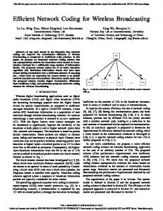
Maximizing Network Lifetime of Broadcasting Over Wireless Stationary Adhoc Networks Intae Kang and Radha Poovendran Department of Electrical Engineering, University of Washington, Seattle, WA email: {kangit,radha}@ee.washington.edu
Abstract— We investigate the problem of energy-efficient broadcast routing over stationary wireless adhoc networks where the host is not mobile. We define the lifetime of a network as the duration of time from the network initialization until the first node failure due to the battery exhaustion. We provide a globally optimal solution to the problem of maximizing a static network lifetime through a graph theoretic approach. We make use of this solution to develop a periodic tree update strategy for dynamic load balancing and show that a significant gain in network lifetime can be achieved. We also provide extensive comparative simulation studies on parameters that affect the lifetime of a network.
I. I NTRODUCTION NE of the important applications of wireless stationary adhoc networks includes wireless sensor networks [2], [4], [6], [14]. The technology of sensor networks has the potential to change the way we interact with our physical environments. For example, inexpensive tiny sensors can be embedded or scattered onto target environments in order to monitor useful information in civilian or military situations. Most of these applications make extensive use of a broadcast model of communications for disseminating data to neighboring sensors. When the communicating wireless nodes are out of reach of one another, they need to rely on intermediate sensor nodes to relay the data back and forth between the sensors [8], [9], [14], [26]. Due to practicality of future applications—ranging from environmental monitoring to national security—and the importance of energy efficiency in this environment, the design of sensor networks has been an active area of research. Special issues of IEEE journals and magazines dedicated to energyefficient adhoc networking problems have been published [1]– [4], [6] in the recent months, serving as excellent sources of new research challenges involved. Wireless communications experience severe attenuation of received signal power due to lossy wireless channel characteristics. Thus, even in the absence of any additional interference, a sender has to ensure that the transmitted signal power level is strong enough for meaningful decoding at the receiver end. A constrained energy source is a salient feature of many of the sensor networks [6]. The (battery) energy of a sensor node is depleted by: (i) computational processing and (ii) transmission/reception of signal to maintain the signal-to-noise
O
A preliminary version of this paper is presented in IEEE ICC 2003 under broadband wireless and satellite communication systems session.
ratio above a certain threshold. While the advances in low power devices can reduce the energy consumption due to computations, the energy consumed by communications is fixed. Therefore, it is essential to develop efficient networking algorithms and protocols that are optimized for energy consumption during communication. Conserving energy is essential since battery depletion will eliminate a node’s ability to continue to communicate. In this paper, we investigate the problem of maximizing the network lifetime of a single broadcast session over a wireless stationary adhoc network, where the network is constrained with strictly limited battery energy resource. Specifically, we first explore the case when the network is not self-configurable, but the initial setup of a routing structure is used throughout the session. Subsequentally, the extension of the solution obtained for static networks to the dynamic (self-configuring) networks is also presented. In broadcast routing [5], [6], [9], [24], which criteria of optimization lead to extended lifetime has not been clearly answered up to now. For example, does the minimization of the total transmit power or maximum transmit power at each instance of time extend the lifetime? If so, which one will perform better? Under what conditions the minimization of maximum transmission power will be optimal? More generally, if the routing structure should be adaptively changed, between minimizing the total cost and minimizing the maximum cost at each instance of time, which one will perform better? These are some of the fundamental questions that need to be addressed. To maximize the lifetime of broadcasting, direct measures natural to the analysis of lifetime should be introduced and the characteristics of wireless broadcast channel should be fully utilized. Our work focuses on evaluating these metrics and characteristic with the goal of determining the optimal strategies in a variety of situations common to wireless adhoc networks. In the case of unicast routing, it has been shown in [7], [11] that the energy-efficiency can be roughly achieved by routing traffic through a path where nodes have sufficient residual battery energy and by avoiding the inclusion of nodes with scarce energy in the path. However, in broadcasting, every node in the network should be included either as a receiver or as a relay node. Hence, an important issue in broadcast routing is to design algorithms with link cost metrics which assign either a very small transmit power or no transmit power (leaf nodes) to nodes with scarce battery energies. In trying to extend the network lifetime, it is critical to
define what we mean by the lifetime of a network. The definition of the network lifetime as the time of the first node failure [11] is a meaningful measure in the sense that a single node failure can cause the network to become partitioned and further services to be interrupted. We use this definition of network lifetime in this paper. We show that the choice of this network lifetime naturally leads to a max-min type (bottleneck) optimization problem, because we want to maximize the time at which the first node failure (minimum) occurs. We model the network as a directed graph and provide a globally optimal solution to the bottleneck optimization problem through graph theoretic approaches. We note that other definitions of network lifetime used in the literature include: (i) fraction of surviving nodes in a network [6], [13], [19], [22] and (ii) mean expiration time [10]. Incidentally, the power-efficient trees defined in [5], [11] do not address the problem of constructing trees with maximum lifetime. In order to do so, we clearly distinguish between the terms power-efficiency (or equivalently short-term energy efficiency e.g., minimum total or maximum transmit power) and energy-efficiency (related to maximizing long-term network lifetime). We then show how to incorporate the residual battery energy in each node to form a suitable cost function for lifetime extension problem. The main contributions of our paper are as follows: 1) For networks that are not self-configurable, we investigated the structure of the most energy-efficient broadcast routing trees that maximize the network lifetime. An optimal solution to this problem is provided using graph theoretic approach. 2) For self-configurable networks, we consider different cost and optimization metrics that extend the network lifetime. Especially, we compare two classes of optimization metrics minimizing for the maximum or total cost and investigate which one is better suited to extend the dynamic network lifetime. 3) We provide comprehensive simulation results and analyse the impact of parameters on network lifetime performance such as tree update interval, network density, path loss factor, initial energy distribution and control overhead. The remainder of this paper is organized as follows. In the next section, we give background and define the terms used in this paper. In Section III, we look at the problem of maximizing static network lifetime without tree updates and the optimal solution is presented. In Section IV, we provide other optimization metrics for comparison. In Section V, the solution obtained is extended to include dynamic lifetime with tree updates and optimization metrics for dynamic lifetime is given in Section VI. Section VII summarizes our simulation results and Section VIII concludes this paper with our future research direction. II. BACKGROUND AND D EFINITIONS In this section, we present the background information and define the fundamental terms used throughout this paper. We note that while most of the needed definitions are presented in
this section, we are forced to present a few deinitions in the next section in order to maintain clarity of the presentation. We assume that each node (host) in a wireless static adhoc network is equipped with an omnidirectional antenna. When the distance between the sender and receiver is d, the received power at a node varies as d −α where α is the path loss (attenuation) factor that satisfies (2 ≤ α ≤ 4). Hence, the transmission power required to reach a node at a distance d is proportional to d α assuming that the proportionality constant is 1 for notational simplicity. To avoid the undue complication of notation, we also assume the receiver sensitivity threshold as 1 (0 dB). Our main focus in this paper is to investigate topology structures (e.g. trees) in the network layer and design cost metrics of links which enable prolonged network operation. Channel contention and retransmissions in MAC or link layers do affect the energy efficiency but, at this stage, are not covered in this paper. We denote a network as a weighted directed graph G = (N, A) with a set N of nodes and a set A of directed edges (links), A = {(i, j)}. For a directed edge (i, j) ∈ A, let π (j) denote the parent node of node j (i.e., π(j) = i), and the weight of the edge is w (i, j). Each node is labeled with a node ID ∈ {1, 2, . . . , |N |}. If it is not specifically stated, we assume that the network is directed. Definition 1 (Static and Dynamic Network): (i) We define a static network as a wireless multihop adhoc network where underlying routing structure is not self-reconfigurable or does not change over time. (ii) When a wireless network is selfreconfigurable or changes over time, we will call it as dynamic network. As an opposite term of mobile network, where the location of hosts changes, we use a term stationary network to avoid confusion. Definition 2 (Pairwise and Node Transmit Power): Given a spanning tree T , the required pairwise transmit power P ij to maintain a link (i, j) ∈ T from node i to j is P ij = dα ij where dij is the distance between the node i and j. The actual (node) transmit power assigned to the node i is PT X (i) = max {Pij } , for i = 1, . . . , N j∈�i
(1)
where �i is a set of adjacent nodes of node i in the tree. Unlike conventional wired networks, there is no permanent connection between the nodes in wireless networks. The transmit power level {P T X (i)} assigned to each node i (and node mobility, if it is a mobile adhoc network) determines the network topology. Definition 3 (Topology): The topology τ by transmit power {PT X (i)} for i ∈ N is a mapping τ : G −→ G� from a directed graph G = (N, A) to a subgraph G� = (N � , A� ) ⊂ G satisfying N � = N and A� = {(i, j) | (i, j) ∈ A(G), Pij ≤ PT X (i)}. Given a transmit power distribution {P T X (i)}, we will call G� as a topology induced by {PT X (i)} [18]–[20]. The topology control problem is to dynamically adjust the transmit power levels to satisfy the specified requirements of applications (e.g., connectivity, strong connectivity, and biconnectivity). For example, if a power assignment fails to
meet the requirement for network connectivity, this leads to the network being partitioned. In general, assigning higher power leads to rich interconnections between the nodes providing many redundant paths but at the cost of larger interference to other nodes and faster battery depletion. On the other hand, by assigning the right amount of power level to maintain the network connectivity, we can reduce the battery consumption rate and hence extend the overall network operation time [5], [6], [18], [21]. In a wireless network, depending on the transmit power assignment, there is always a trade-off between reliability (fault tolerance) and network lifetime. There exists a whole spectrum of topology control problems in between. At one extreme, there is flooding with maximum transmit power (uncontrolled topology) where a network is most reliable at the cost of minimal network lifetime [25]. The other extreme is a spanning tree. Since a spanning tree is the minimal graph structure supporting the network connectivity, it is intuitively clear that a topology which maximizes the network lifetime under transmission should be a tree. But any tree-based scheme comes at the cost of relatively weak link connectivity, because a single node or edge failure results in network partition. A tree-based approach is suitable for the networks where the topology change is not frequent, such as wireless sensor networks. Definition 4 (Arborescence): For a directed weighted graph (network), a directed spanning tree rooted at a node is called an arborescence (or a spanning branching) [32]–[34]. A branching B of a directed graph G is defined in [33] as follows: (i) If (x1 , y1 ), (x2 , y2 ) are distinct edges of B, then y 1 �= y2 , (ii) B does not contain a cycle. One of the main objective in this paper is to construct a broadcast routing tree 1 rooted at the source node with the longest possible lifetime. In broadcast routing, a message originating from the source node should reach every destination node. Definition 5 (Network Connectivity): We define that a network is connected if there exists a directed path denoted as (S � i) from the source node S of the broadcast to every destination node i in the network. The network connectivity in this paper is equivalent to the strong connectivity (or reachability) from the root (source) node. Furthermore, the connectivity does not require duplex links, namely, if there is a directed edge (u, v) ∈ (S � i) , it is not necessary for an edge (v, u) to exist. The connectivity of a network can be easily represented with an |N | × |N | adjacency matrix A = [a ij ], where aij = 1, if there is a link between node i and j, and a ij = 0, otherwise. In addition, we assume that the graph is loop-free so that the diagonal entries of A are zero (i.e., a ii = 0 for all i ∈ N ). In general, the adjacency matrix is not symmetric for a directed graph (digraph). Without loss of generality, we assume that the source node ID is 1 and, hence, the first row of A represents the connection from the source node. For a network of size 1 Unless otherwise mentioned, a tree in this paper means an arborescence from now on.
|N |, we denote the connectivity matrix [35] as: C = A + A2 + · · · + A|N |−1 .
(2)
If the non-diagonal entries of the first row of C are nonzero (i.e., c1j > 0 for j = 2 . . . |N |), the network is said to be strongly connected from the source node to every destination node. Practically, the test for connectivity is done using the standard depth-first search (DFS) algorithm [17] which has a running time of Θ (|V | + |A|). Definition 6 (Physical and Logical Neighbor): If a node i is transmitting with power P T X (i), then the physical neighbor ℵi of node i in a wireless network is a set of all the nodes within the communication boundary ℵi = {k | 0 < Pik ≤ PT X (i)} .
(3)
The logical neighbor � i of node i is a set of adjacent nodes �i = adj (i) = {k | π(k) = i} .
(4)
In general, the physical neighbor determined by a network topology and transmit power does not coincide with the logical neighbor determined by a routing algorithm, and usually � i ⊆ ℵi . Further implications of the difference of physical and logical neighbor will be discussed in Section II-A. Definition 7 (Network Lifetime): Given a broadcast routing tree T , (i) the network lifetime L (T ) is defined as the duration of the network operation time until the first node failure due to battery depletion at the node, assuming that broadcast from the source node takes place at the beginning of the network initialization. (ii) The static network lifetime refers to the lifetime when the tree T does not change once the tree is setup at the initialization phase. (iii) The dynamic network lifetime refers to the case when the tree T is updated based on an update policy (for example, either periodically or whenever there are changes in the network topology). First, let’s concentrate on the static network case. Because the routing tree does not change over time, the transmit power PT X (i) determined by (1) is not a function of time. Whenever there needs to emphasize the time-varing nature of transmit power as in dynamic networks, we will use the notation PT X (i, t). If the current battery energy level of node i at time t is Ei (t) and the node i is using transmit power P ij to transmit to node j, this link can be used for the remaining Ei (t) /Pij units of time. Definition 8 (Link and Node Longevity): We define the link longevity lij of a link (i, j) ∈ T as lij ≡
Ei (0) . Pij
(5)
The node longevity � i of a node i ∈ N is defined as follows: �i ≡ min {lij } = j∈�i
Ei (0) Ei (0) = , max {Pij } PT X (i)
(6)
j∈�i
where �i is the set of logical neighbors of node i and P T X (i) is the actual (node) transmit power assigned to the node i. Both link and node longevity have time as their dimension. A node i transmitting data with power P T X (i) can live for � i units of time. If a node i is a leaf node in the spanning tree,
then PT X (i) = 0 and thus �i = ∞. Otherwise, the source and relay nodes have a finite node longevity. Note that, given a spanning tree T with node i transmitting with power P T X (i) given by (1), the total transmit power of this tree is � PT X (T ) = PT X (i) . (7)
5
4
8
l 34=7s
◦
We denote a tree with minimum total transmit power as T � T ◦ = arg min PT X (T ) = arg min PT X (i) . (8)
l 13=8.5s
6 l 16=1s
Source
7
1 l 12=9s
T ⊂G(N,A) i∈N
The residual battery energy E i (t) at time t is related to PT X (i, t) as follows2 � t Ei (t) = Ei (0) − PT X (i, τ ) dτ. (9)
l 68=2s
l 67=3s
3
i∈N
T ⊂G(N,A)
l 45=25s
2 Fig. 1. node.
A sample network configuration: the node with ID=1 is the source
0
Note that we do not consider in our battery model the nonlinear behavior of voltage as a function of remaining capacity [7] or the battery charge recovery effect due to diffusion process [38], [39] but use a simplified linear battery discharge model. We intend to study the effect of different battery models in the future. In a static network case, given an initial distribution of current battery energy levels {E i (0)} and the transmit power levels {PT X (i)} determined by a routing algorithm, the static network lifetime of a connected tree T induced by {P T X (i)} is related to the link and node longevity as follows: � � Ei (0) (10a) L (T ) ≡ min = min {�i } i∈N i∈N PT X (i) � � (10b) = min min lij = min {lij } , i∈N
(i,j)∈A(T )
j∈�i
where A (T ) is the edge set induced by a tree T . Hence, the network lifetime of a tree T is determined by a node with the minimum node longevity, which in turn depends upon a link with the minimum link longevity. Definition 9 (Bottleneck Edge): Let’s denote the maximum edge weight of a spanning tree T ⊂ G (N, A) as µ (T ) ≡
max
(i,j)∈A(T )
w (i, j)
and we will denote the edge (i, j) satisfying this condition as the bottleneck edge. Definition 10 (Bottleneck Spanning Tree): A Bottleneck Spanning Tree (BST) denoted as T BST is defined as a spanning tree which has the minimum bottleneck edge weight: TBST ≡ arg min µ (T ) . T ⊂G(N,A)
(11)
�Definition 11 (Energy Pool): The sum of all node energies i∈N Ei (t) at a given time t is defined as the energy pool of the network at time t. Now, we will provide a few examples on how these definitions can be applied to different scenarios. Example 1: Fig. 1 gives a sample instance of a network configuration where node IDs and link longevity values are 2 In this paper, we investigate the energy consumption by transmit power only. A more general, hence precise, formula can be found in (13).
displayed next to the corresponding nodes and edges. In this example, the network lifetime is determined by the edge (1, 6) because the link longevity (5) of the edge has the minimum value l16 = 1 sec. The node longevity (6) for the source and relay nodes are � 1 = 1 sec, �3 = 7 sec, �4 = 25 sec and �6 = 2 sec. The leaf nodes 2,5,7 and 8 have infinite node longevity. From this example, we note that the lifetime extension problem can be formulated as a bottleneck optimization problem [36]. Example 2 (Equally Distributed Energy Network (EDEN)): As a special case, when the nodes of a network have identical initial energy levels (i.e., E 1 (0) = . . . = E|N | (0) = E), we will denote the network as an equally distributed energy network (EDEN). The lifetime of EDEN can be expressed as: LEDEN (T ) =
E max
(i,j)∈A(T )
{Pij }
.
(12)
This scenario roughly simulates the real situation where, at the beginning of a conference session, attendees try to bring their laptop fully charged. It is assumed that the battery capacity of each host is the same. Example 3 (Flooding): Another common example is flooding [25]. Although we concentrate on the network lifetime for a tree, the definition (10a) is applicable to any general topology. In flooding, each node caches the messages it has previously received. If a message currently received is in the cached list, it simply drops the message. Otherwise, it retransmits the message with maximum available power P max . Hence, each node transmits each message exactly once even though it can receive the same message multiple times. In this case, the network lifetime for flooding is: �
E|N | (0) E1 (0) ,..., Pmax Pmax mini∈N {Ei (0)} , = Pmax
�
Lf looding = min
assuming each node is equipped with the same radio transceiver, i.e., P T X (i) = Pmax for all i ∈ N.
A. Computation of Receive Power and Interference Level The following RF and computational components [12], [13] contribute to the battery energy drain: PT X (i, t) : RF transmit power of node i at time t pT X (i) : transmit signal processing power of node i pRX (i) : receive signal processing power of node i , pc (i) : other information processing power of node i where pT X (i), pRX (i) and pc (i) correspond to the power consumption by computational signal processing and the RF component P T X (i, t) corresponds to the power consumption mainly due to power amplifier circuitry (PLL, VCO, etc.) for transmission with an antenna. The transmit signal processing power pT X (i) is due to modulation, encoding and encryption, and the receive signal processing power, or simply receive power, pRX (i) is for signal reception such as equalization, demodulation, decoding and decryption. p c (i) is related to all other signal processing power for data processing other than for communications at the node. We assume that each computational component of every transceiver is the same (pT X (i) = pT X , pRX (i) = pRX and pc (i) = pc for all i). Considering all the components introduced above, a more realistic model of energy dissipation will be � t Ei (t) = Ei (0) − [PT X (i, τ ) + pT X ] IT (i, τ )dτ � t� 0 � t (13) − IR (i, j, τ ) pRX dτ − pc dτ 0 j∈N
0
where IT (·) and IR (·) are indicator functions such that � 1, if i is transmitting at time t IT (i, t) = 0, otherwise � 1, if i ∈ ℵj at time t IR (i, j, t) = . 0, otherwise Given a routing tree structure, the source and relay nodes are transmitting nodes and the leaf nodes are receiving nodes. Definition 12 (Total Receive Power): Assuming p RX (i) = pRX for i ∈ N , the total receive power P RX (T ) of a network is �� � PRX (T ) = pRX (i) = pRX |ℵj | , (14) j∈N i∈ℵj
j∈N
where ℵj is the physical neighbor of node j determined by the node transmit power P T X (j) and the network topology. Note that ℵj = ∅ when PT X (j) = 0. Because there are (|N | − 1) receivers in broadcasting, the only portion of receive power meaningfully processed by the receivers is (|N | − 1) pRX . Hence, the amount of power expenditure due to unnecessarily processing the signal is � (|ℵj | − |�j |) pRX PRX (T ) − (|N | − 1) pRX = j∈N
=
�
�
pRX ,
(15)
j∈N i∈ℵj \�j
where ℵj \�j represents the set difference operation. Note that every received packet should be processed (sometimes) up to
Fig. 2. Receive power and interference: dashed lines represent the mismatch between physical and logical neighbors.
application layer either to determine the next hop destination for forwarding, or to accept and further process the data (or simply drop). When a node i transmits signal with transmit power PT X (i), the actual received power at node j is P (i) /d α ij due to channel attenuation. Definition 13 (Total Interference Power): With a current transmit power assignment {P T X (i)}, the total interference power at node j is the sum of all received power: � PT X (i) /dα (16) ij . i∈N \{j∪π(j)}
Among these, what is more detrimental to correct signal reception is the received power whose signal strength is larger than the receiver threshold (0 dB in this paper), because it is a data-like interference (or crosstalk) [16]. We will call this quantity, closely related to (15), as the total effective interference power level � � PT X (i) (17) PI (T ) = dα ij i∈N j∈ℵi \�i
The total effective interference power corresponds to cochannel interference and hence directly affects the performance in bit error rate (BER) in lower layers. Therefore, in designing a network routing algorithm, it is important to make the mismatch between physical and logical neighbors smaller to reduce not only the total receive power but also total effective interference. Example 4: In Fig. 2, a sample broadcasting routing tree for a network with 10 nodes is shown. The number of dashed lines (4, in this example) represents (|ℵ j | − |�j |), and the amount of wasted receive power due to unnecessary signal processing (15) is 4 · pRX and total effective interference power (17) is α α α PT X (1) /dα 12 + PT X (9) /d91 + PT X (5) /d53 + PT X (5) /d57 . It was shown in [21] that the receive power of the current generation of RF devices can take as much as a half of transmit power. Therefore, the power consumption from the signal reception can significantly affect the network lifetime (e.g., especially in flooding). This implies the importance of an intelligent dedicated radio hardware which can redirect the network traffic within the communication subsystem without having to go through CPU [37], [40].
We are not aware of any solution that simultaneously optimizes both transmit and receive power using (13). However, the receive power is determined by the transmit power assignment. Hence, we can still analyze the impact of transmit power assignment on receive power and interference level. It will be presented by simulations in Section VII (see e.g., Fig. 10 and 11). From these results, we can roughly estimate the BER performance of each routing algorithm in lower layers. III. M AXIMIZING S TATIC N ETWORK L IFETIME In this section, we investigate an optimization problem of finding a routing (spanning) tree which maximizes the network lifetime without tree update. We assume that once a routing tree is established at the beginning of a broadcast session, the same tree is used as a broadcast routing tree for the whole remaining time. We want to find a static routing tree T ∗ which gives the maximum network lifetime. Definition 14: The (globally) optimal static network lifetime L∗ is defined as L∗ ≡ =
max
{L (T )}
max
min
T ⊂G(N,A)
T ⊂G(N,A) (i,j)∈A(T )
(18a) {lij }
(18b)
where lij is the link longevity of an edge (i, j). This max-min (bottleneck) optimization problem (18b) is a network design problem which finds an optimal power assignment to each node by finding an optimal spanning tree. We will show in the following subsections that we can, in fact, find a (global) optimum solution to this problem by polynomial-time bounded greedy algorithms. A. A special case (EDEN)—undirected graph We initially look at a special case (Example 2) when all the nodes have identical battery energy levels. Although this constraint is possibly too stringent in real situations, we solve this problem first because it provides insights into the more general case of unequal battery energies. Due to this equal energy assumption, the graph can be considered as undirected because lij = E/Pij = E/Pji = lji . First, we will derive a lemma which will be used later. In deriving this, we use the cut optimality of a minimum spanning tree [17]. Lemma 1 (MST minimizes the bottleneck edge weight): Let µ∗ denote the minimum of µ (T ) over all possible spanning trees of a weighted undirected graph, i.e., µ∗ ≡
min
T ⊂G(N,A)
{µ (T )} .
(19)
If we denote the Minimum Spanning Tree (MST) as T MST , then (20) µ (TMST ) = µ∗ . Proof: We make use of definitions (9) and (10) in this proof. This problem can be rephrased as proving that a minimum spanning tree is also a bottleneck spanning tree. The following three cases are considered in our proof. First, the case µ (TMST ) < µ (TBST ) is not possible by the definition
(11), since µ (T BST ) = µ∗ . Now, suppose that the minimum spanning tree is not a bottleneck spanning tree, then µ (TMST ) > µ(TBST ) = µ∗ .
(21) ∗
Now, denote the bottleneck edge of T MST as e = arg max(i,j)∈TM ST w (i, j). Removing this edge e ∗ ∈ TMST introduces a cut C, which is by definition a partition of a node set N into two nonempty subsets N 1 and N2 or, equivalently, a set of edges connecting N 1 and N2 , i.e., C = {(i, j) ∈ A|i ∈ N1 , j ∈ N2 }. Note that since TBST is a tree, exactly one edge e ◦ ∈ TBST should be included in the cut C so that connectivity of a tree can be satisfied (e ◦ is not necessarily the bottleneck edge of T BST ). By the cut optimality of a minimum spanning tree [17], we know that w (e∗ ) ≤ w (e◦ ). Therefore µ (TMST ) = w (e∗ ) ≤ w (e◦ ) ≤ µ (TBST ) .
(22)
This leads to a contradiction with (21). Therefore, the only possible case is µ (TMST ) = µ (TBST ). Thus, every minimum spanning tree is also a bottleneck spanning tree. Lemma 1 proves that a minimum weight spanning tree is a sufficient condition to be a bottleneck spanning tree. However, it is not a necessary condition in general, which can be simply proved with a counter example [17]. Hence, MST is a globally optimal solution but not unique. In fact, any tree with the same maximum weight edge (bottleneck spanning trees) serves our purpose equally well. Theorem 1: If all the nodes in a network have identical battery energy E, then the minimum spanning tree is a globally optimal solution to the static network lifetime maximization problem. Proof: If we use the edge weight w (i, j) = P ij = dα ij , then w (i, j) = w (j, i) because dij = dji and the network is modeled as an undirected graph. Hence, Lemma 1 is applicable. Using (12), (18a), and (19), the (global) maximum lifetime L∗ is L∗ =
max
LEDEN (T ) 1 = E · max max T ⊂G(N,A) T ⊂G(N,A)
(i,j)∈A(T )
Pij
E minT ⊂G(N,A) max(i,j)∈A(T ) Pij E . = µ (TMST ) =
Since µ (TMST ) = µ∗ is minimum among all possible spanning trees by Lemma 1, the maximum lifetime L ∗ is obtained by using a minimum spanning tree with cost metric w (i, j) = Pij and is also globally optimal. Corollary 1: Minimizing the total pairwise transmit power gives the optimal solution to the static lifetime maximization problem only when the network is equally energy distributed (EDEN). Proof: By definition [17], MST is a spanning tree with minimum total cost: � w (i, j) . (23) TMST = arg min T ⊂G(N,A)
(i,j)∈A(T )
a
K
S Fig. 3.
1
K-1
K-1
b
Illustration for Lemma 2.
If we use w (i, j) = Pij , a pairwise transmit power, it is obvious by Theorem 1. We strongly emphasize that MST is not a tree with minimum total transmit power (7) and does not exploit the wireless broadcast advantage property during its construction as in [5]. In general, when there exist links with equal weights (costs), minimum spanning tree is not unique. However, when the weights are distinct, the minimum spanning tree is unique [17]. This uniqueness property facilitates the implementation of a distributed algorithm for MST [15], [31]. B. General case—directed graph Once we begin to consider the general distribution of the residual battery energy levels (i.e. there exist i and j such that Ei (t) �= Ej (t)), the graph is no longer undirected. Note that w (i, j) = Ei (t) /Pij and w (j, i) = Ej (t) /Pji . Hence, although Pij = Pji , w (i, j) �= w (j, i). Finding a minimum weight arborescence (branching) (Definition 4) has exactly the same formula as undirected one (23), except that the underlying graph is changed to a directed one [31]–[34]. Therefore, a minimum weight arborescence is conceptually a direct extension of MST for a directed case with the same underlying optimization principle. In Section III-A, we found that a global optimal solution for EDEN is MST and then obtained an important result that minimization of the total cost leads to minimization of the maximum cost for an undirected graph (but not vice-versa). It is natural to ask the question whether this analogy carries over to a directed graph as well. Unfortunately, the answer is negative and a proof is provided, which is due to Khuller [30]. Lemma 2: Minimum (total) weight arborescence rooted at the source node does not necessarily minimize the maximum weight of a directed graph. Proof: This can be easily verified with the following counter example. Consider the configuration in Fig. 3 with a node set N = {S, a, b}. The edge weights are shown in Fig. 3 next to the directed edges, where K > 3 is assumed. The minimum weight branching rooted at S is {(S, a), (a, b)} of total weight K + 1 and maximum weight K. The branching minimizing the maximum weight of any edge is {(S, b), (b, a)} with total weight 2(K − 1) and with maximum weight K − 1. Although the total weight is smaller (K + 1 < 2 (K − 1)), the maximum weight is larger (K > K − 1) . Therefore, the min-
imum weight arborescence does not minimize the maximum weight of a directed graph. Thus, the results for undirected graph in Lemma 1 cannot be directly applied to a directed graph and we need to solve a new bottleneck optimization problem similar to Lemma 1 for a directed graph. We will show that there is a polynomial-time bounded algorithm that will compute what we need. Algorithm 1: Consider S as a sorted set of weights on edges in an increasing order. Let τ i be the topology (subgraph) formed by the first i edges in S. Check if τ i has the property that the root can reach every node. If so, we can discard all the edges with index larger than i. We are looking for the smallest i for which this property holds. We can do binary search to find this i, since there is some value j such that τ j does not have this property and τ j+1 does [30]. Because this algorithm finds the first edge which makes the graph connected chosen from the ordered edge weights, it is clear that this algorithm will give us a desired optimal solution (i.e., the bottleneck edge weight of a directed graph). The computational complexity of Algorithm 1 is polynomial-time bounded, Θ ((|V | + |A|) log |A|), since the worst cast running time Θ (log |A|) factor of the binary search is added to a linear time Θ (|V | + |A|) connectivity test using the standard depth first search (DFS) algorithm. Algorithm 2 (DMST): By applying Algorithm 1, a topology τj can be found where all the edge weights are upper bounded by the bottleneck edge weight. We applied Prim’s algorithm [17] on τj rooted at the source node by inspecting only outgoing edges at each step. We will call this algorithm as a directed minimum spanning tree (DMST). The difference between Algorithm 1 and 2 (DMST) is that Algorithm 1 finds a connected topology, whereas DMST finds a connected arborescence. It is intuitively clear that DMST has the same bottleneck edge as Algorithm 1, since otherwise the arborescence cannot be connected. Therefore, DMST finds the minimum of the maximum edge weight out of all possible arborescences. Theorem 2: Let w (i, j) be the inverse of link longevity (or normalized pairwise transmit power): −1 = w (i, j) = lij
Pij , Ei (t)
(24)
then DMST is a (globally) optimal broadcast routing tree solution of static network without tree update. Proof: Applying Algorithm 1 and 2 on a directed graph leads to an arborescence that minimizes the maximum edge weight among all possible arborescences. From (24), DMST has the minimum of the maximum P ij /Ei (t). Equivalently, it has the maximum of the minimum link longevity l ij . Since the globally optimal network lifetime is (18a), this proves that DMST can achieve global optimality in maximizing the general static network lifetime. An interesting consequence of this result is that the network lifetime, which is a global property of the network, is determined by node longevity, which is a local property of the network.
IV. M ETRICS FOR S TATIC L IFETIME P ERFORMANCE C OMPARISON A. Maximum Static Network Lifetime (MSNL)—DMST This metric corresponds to the Algorithm 2 (DMST) in conjunction with link weight w (i, j) = P ij /Ei (t). It is proven to be optimal for static network.
If we label every node in ℵ i as ik in an increasing order of distance from node i (i.e., i = i 0 , i1 , . . . , i|ℵi | such that Piip < Piiq if p < q), then the transmit power P T X (i) of node i can be represented as the sum of incremental power |ℵi |−1
PT X (i) =
�
∆Piik ik+1 .
(26)
k=0
B. Minimize Maximum Transmission Power (MMTP)—MST We note that although this is one of the well studied metrics in the literature [7], [10], [18], the cases for which it performs well have not been clearly presented. We have proved in Section III-A through a graph theoretic approach that: • this metric corresponds to MST (or BST) with weighting function w (i, j) = Pij , • this metric can be optimal only for undirected graphs. Therefore, this metric is equivalent to MSNL only for EDEN. • in other general cases (Section III-B, V), the solution obtained by this metric is not optimal.
Substituting (26) to (8) leads to ◦
T = arg min
i |−1 � |ℵ�
T ⊂G(N,A) i∈N k=0
∆Piik ik+1 .
(27)
Hence, the total transmit power is the same as the total incremental power. The BIP algorithm [5] effectively solves (27) to find a solution to (8). As noted earlier, finding an optimal solution to minimum total transmit power is NP-hard and BIP in Fig. 4 is the best known heuristic greedy algorithm for this3 . As is clear from (8), there is no time-dependence in the equation and, hence, BIP is an algorithm for a static tree. V. M AXIMIZING DYNAMIC N ETWORK L IFETIME
C. Minimize Total Transmit Power (MTTP)—BIP It was shown in [23], [28], [29] that the construction of minimum total power broadcast routing tree with limited power is NP-hard. However, there is a suboptimal centralized algorithm called Broadcast Incremental Power (BIP) [5] that uses a greedy approach to construct a power efficient tree. The details are given below for reader’s convenience. BIP A LGORITHM Input: an undirected weighted graph G = (N, A) Initialization: T := {S} where S is the source node PT X (i) := 0 for all i ∈ N Procedure: while (|T | �= |N |) find an edge (i, j) ∈ T × (N \T ) such that incremental power ∆Pij = Pij − PT X (i) is minimum. T := T ∪ {j}, A(T ) := A(T ) ∪ {(i, j)} PT X (i) := PT X (i) + ∆Pij Fig. 4.
BIP algorithm: a heuristic greedy algorithm
Due to the broadcast nature of the wireless medium for omnidirectional antenna, a unit of message sent to receiver R at the boundary of the transmission range reaches every node within the range for “free.” Therefore this property is called “wireless broadcast advantage” [5]. The BIP algorithm of Fig. 4 uses the wireless broadcast advantage property while growing a tree. This algorithm is similar to the Prim’s algorithm for MST and hence the computational complexity is roughly equivalent. Let Pij be the power required to reach node j from node i and node k is further apart (P ik > Pij ) from node i. The i incremental power ∆Pjk of node i is defined as the additional power required to reach another node k [5]: i ∆Pjk = Pik − Pij .
(25)
From now on, we look at the problem of maximizing dynamic network lifetime introduced in Definition 7. We assume that every network is modeled as a directed graph. We now define the optimal lifetime for dynamic networks. Definition 15: The optimal dynamic network lifetime L ◦ is defined as L◦ = max min {�i } (28) {PT X (i,τ )} i∈N
subject to � � {PT X (i, τ )} induces a connected topology at each instance of time τ ≤ L ◦ where �i satisfies � �i PT X (i, τ ) dτ = Ei (0) for all i ∈ N.
(29)
(30)
0
Note that �i in (30) corresponds to the node longevity for dynamic network lifetime analogous to (6) for a static case. The problem of maximizing the dynamic network lifetime is equivalent to finding a set of time-dependent transmit power {PT X (i, τ )} which gives a connected topology at any time τ . Example 5: One sample instance of this problem is illustrated in Fig. 5 where the transmit power of each node is shown as a function of time. Each curve in this figure does not vary continuously but rather takes discrete values, because we assume that each node transmits with power just enough to reach other nodes. Also the area under each curve corresponds to the initial energy of each node. In this example, the dynamic network lifetime is determined by node 2 which has the minimum node longevity. Ideally, given an initial energy distribution {E i (0)} and the location of each node, {P T X (i, τ )} can be calculated off-line, because these are all the information we need. However, we are not aware of any method to solve this problem analytically 3 We note that another suboptimal algorithm called EWMA [41] was developed which has a distributed implementation.
PTX(1)
P
E1
(2)
TX
E
2
.. . P
(|N|)
TX
E
|N|
t
�2 Fig. 5.
�|N | �1
Illustration for dynamic network lifetime
in a close form. As implied in Fig. 5, the optimal solution to the dynamic network lifetime problem is not a function of a single tree anymore but it is a function of a series of trees: L = L (T (0) , T (t1 ) , T (t2 ) , ...) . It is still an open problem what is the maximum theoretically attainable dynamic lifetime. Instead, we take a greedy, online approach by making a best effort to optimize for certain criteria (e.g., minimize maximum or total cost) at each instance of time. In this case, what kind of optimization criteria (hence, resulting trees) should be used, and when and how often the trees should be updated are the important issues. We note that neither minimizing the maximum transmit power (MMTP) nor minimizing the total transmit power (MTTP) discussed in Section IV is a valid figure of merit anymore for dynamic networks. Both MMTP and MTTP depend entirely on the location of nodes and hence the current residual battery energy has no effect on the constructed trees. In this regard, finding any static (time-independent) tree, whether optimal or not, is not sufficient, since a single node with minimum node longevity determines the network lifetime. This incurs a premature death of a network regardless of how much energy still remains at other nodes. In a self-reconfigurable (dynamic) network, the optimality of the static network lifetime discussed in the prior section does not last long. For instance, given an energy distribution {Ei (t)} at time t, suppose an optimal spanning tree T (t) is constructed by DMST algorithm with edge weights w (i, j) = −1 = Pij /Ei (t) and it is used as a broadcast routing tree for lij a period of time ∆t. The energy distribution at time t + ∆t changes to {Ei (t + ∆t)} = {Ei (t) − ∆t · PT X (i)}. Because the edge weights change to P ij /Ei (t + ∆t), the bottleneck edge weight µ (T (t)) can change and hence the optimality of static network lifetime does not hold true anymore. However, temporal optimality in lifetime can be reclaimed with the following strategies: • triggered update: whenever the bottleneck edge changes, the tree is updated. • periodic update: instead, we can take a proactive approach to update the tree at every specified interval ∆t. In this paper, we will exclusively use the periodic update strategy and investigate what is the best optimization criterion
at each time interval. If the update interval is larger than the static network lifetime (∆t ≥ L ∗ ), the dynamic network lifetime is equivalent to the static network lifetime. By incorporating the residual battery energy into cost metric, the routing structure can be randomized over time even for a stationary network. Therefore, we can perform loadbalancing [7], [13] by distributing energy dissipation evenly among the nodes throughout the network operation time and extend network lifetime. In effect, load-balancing of battery energy makes the network lifetime less dependent on a specific initial energy distribution and what becomes more important is the whole amount of energy in the network. Because of the dynamic nature of this problem, conceptually, what we want to achieve is fully and efficiently utilizing the energy pool with minimum power for network connectivity. In order to provide an absolute measure of comparison among different optimization metrics, we propose an upper bound to the optimal dynamic network lifetime as follows. Lemma 3: An upper bound to the optimal dynamic network lifetime L◦U is � � i∈N Ei (0) i∈N Ei (0) ◦ �� �, = LU ≡ (31) ◦ PT X (T ) min i∈N PT X (i) T ⊂G
where the numerator represents the initial energy pool of the network. Proof: Assuming recharging the battery is not an option, we cannot spend energy more than the initial energy pool � E (0). Also, to form a routing (spanning) tree, no i i∈N matter what kind of tree we use at each update interval, at least PT X (T ◦ ) amount of power should be spent. Hence, the dynamic network lifetime cannot exceed this upper bound L ◦U . Lemma 4: The optimal static network lifetime L ∗ is strictly upper bounded by L ◦U , i.e., � � � � �� � Ei (0) Ei (0) max min < max � i∈N (32) T ⊂G i∈N T ⊂G PT X (i) i∈N PT X (i) Proof: Let a = (a1 , . . . , an ) be a sequence of positive numbers and b = (b 1 , . . . , bn ) be a sequence of nonnegative numbers where there is at least one nonzero element such that bj �= 0 for 1 ≤ j ≤ n and also there is at least one zero element such that b k = 0 for 1 ≤ k ≤ n. If m = mink { abkk } = min { abkk }, then we have successively for all 1 ≤ k ≤ n
k,bk =0
0 < mbk ≤ ak , if bk �= 0 0 = mbk < ak , if bk = 0 n n � � m bk < ak k=1
k=1
and because there is at least one nonzero element in b, � n k=1 bk �= 0. Hence �n ak ak < �k=1 . (33) min n 1≤k≤n bk k=1 bk Given a routing tree T in a directed graph G, there exists at least one leaf node (with zero transmit power). {P T X (i)}
L1 L2 L3 k j1
j2
j3
D1 D2 D3
L4
(a) a tree before post sweeping
L1 L2 j1 j2 j3 k
L3
D1 D2
L4
D3
T OP -D OWN -P OSTSWEEP l := 1 while (l < h) 1 for each i ∈ Ll if (�i �= ∅) do 2 for each k ∈ Di do 3 if (�k = ∅, k ∈ ℵi ) � � 4 PT X (π (k)) := max Pπ(k),m | m ∈ �π(k) 5 π (k) := i 6 elseif (�k �= ∅, k ∈ ℵi ,�Pin < PT X (i) for ∀n�∈ �k ) 7 PT X (π (k)) := max Pπ(k),m | m ∈ �π(k) 8 π (n) := i for ∀n ∈ �k 9 π (k) := i 10 PT X (k) := 0 11 l := l + 1 Fig. 7.
Top-down postsweep algorithm
(b) resultant tree after top-down post sweeping Fig. 6.
Abstract trees showing the parent-child relationships.
can be calculated by (1) from the tree T . Also for the graph G to be connected, there is at least one node with nonzero transmit power. Let a i = Ei (0) and bi = PT X (i), then these satisfy the condition for a and b. Because the inequality (33) holds for arbitrary trees, (32) immediately follows. Because the upper bound L ◦U does not contain the notion of first node failure, we can presume that it is a quite loose upper bound to dynamic network lifetime. As mentioned before, finding a broadcast routing tree T ◦ with minimum total transmit power with limited power is NP-hard. Thus, both (31) and (8) are not achievable with polynomial-time bounded algorithms. We will approximate the denominator in (31) with BIP algorithm, currently the best known approximation, in our simulation.
A. Post Sweeping—A Heuristic Optimization Technique The total transmit power (7) can sometimes be further reduced by post sweep procedure described in [5] which is a heuristic prune-and-graft technique. Similar idea can be found in [18] as perNodeMinimalize procedure, where binary search technique of depth first search is extensively used. The post sweep procedure essentially removes redundant hops using the wireless broadcast advantage property and thus saves power expenditure. It is not tied to a specific routing algorithm but can be used in conjunction with arbitrary trees. In [5], a random post sweep method was proposed. We propose a heuristic top-down approach based on the observation that, since the underlying data structure is a tree, a more systematic approach can be developed independent of the ordering of the node ID. Other variations such as bottom-up approach are also possible. An advantage of top-down approach is the hop counts to destination nodes always decrease. In terms of the conventional performance measure, this corresponds to better delay characteristic because nodes can be reached within fewer
hops. We use this approach in favor of smaller delay and no optimality is claimed. Fig. 7 describes the implementation of our top-down post sweep procedure. Let L l denote the set of all nodes at level l and Dl denote the set of all node at levels higher than l (i.e., Dl = Ll+1 ∪ Ll+2 ∪ . . .). For any node i at tree level l, every node until the maximum level h is examined (bounded region within dashed line). If a leaf node (e.g., node k) is in the transmission range of node i (line 3), the node becomes a child node of node i regardless of its previous parent node. If a relay node (e.g., node j) and all its neighbor nodes (e.g., jk ∈ �j ) lie within the communication boundary of node i (line 6), direct links are established from the node i to j and jk (k = 1 . . . |�j |). This implies that the transmission by node j is redundant and waste of power and, hence, it can be safely eliminated without disrupting connectivity (line 10). Also it is possible that parent nodes of j and k can reduce the transmit power if j and k are the farthest nodes of � j and �k from π (j) and π (k), respectively. Hence, the total transmit power PT X (T ) can be reduced in line 4, 7, and 10. Fig. 6(a) represents a routing tree showing the parent–child relationships. If the top-down post sweep algorithm is applied at node i in Fig. 6(a), the final result is Fig. 6(b), where node j, k and j1 , j2 , j3 become child nodes of node i. This operation is repeated from the source (root) node down to every node in the sublevels except for leaf nodes. The post sweep procedure will be used in conjunction with other cost metrics to further extend the network lifetime in Section VI and VII. Also notice that the post sweeping does not affect the static network lifetime.
VI. M ETRICS FOR DYNAMIC L IFETIME P ERFORMANCE C OMPARISON In this section, we present different metrics/algorithms to give baseline measure of performance comparison for dynamic network lifetime. We will introduce four dynamic routing trees. Similar ideas can be found in [7], [10], [13].
A. Minimize Maximum Transmission Cost (MMTC)—WMST This metric corresponds to the best effort (greedy) approach to extend the lifetime by maximizing the static network lifetime at each update interval. At every update interval ∆t, a snapshot of tree T MSN L (t) by the MSNL is made. The transmission cost in this metric represents the inverse link longevity Pij . (34) w (i, j) = Ei (t) By using MST algorithm with this cost metric at time t, we essentially solve the following optimization problem � � �� Pij TW MST (t) = arg min max , (35) Ei (t) T ⊂G(N,A) (i,j)∈T where t = k∆t for integer k and the time dependence of this tree is emphasized. In fact, this algorithm covers a class of cost metrics (Pij /Ei (t))µ where µ > 0, because xµ for µ > 0 is a monotonic increasing function of x and MST algorithm only depends on the ordering of link weights. Hence obtained trees are identical regardless of the value µ. We will call the class of algorithms with these cost metrics as Weighted MST (WMST). In a different perspective, the time-dependent weighting function (34) includes both node-based and link-based cost, where Ei (t) is a node-based cost because the battery energy is a characteristic of each node. On the other hand, P ij is a link-based cost because different values are assigned for each link (i, j). As battery energy is being depleted, a higher cost to all the edges incident on the node are assigned so that the node either can be assigned a small power level or can be a leaf node requiring no transmission. B. Minimize Total Transmission Cost (MTTC)—WBIP This metric corresponds to the best effort (greedy) approach to extend the network lifetime by minimizing the total transmission cost at each update interval. We denote the algorithm corresponding to this metric as Weighted BIP (WBIP). A timedependent (dynamic) tree at each instance of time is found with the following optimization formulation: TW BIP (t) = arg min
i |−1 � |ℵ� ∆Piik ik+1
T ⊂G(N,A) i∈N k=0
Ei (t)
.
(36)
The modified cost metric in this case is the incremental inverse link longevity instead of the incremental power (25) −1 −1 i lik (t) − lij (t) = Pik /Ei (t) − Pij /Ei (t) = ∆Pjk /Ei (t) .
Considering this cost as a normalized transmit power, the computational complexity of finding minimum total transmit cost should be at least as large as that of BIP algorithm for total transmit power, and hence the exact optimal solution cannot be found in polynomial time. We approximate this problem with the algorithmic description Fig. 4 along with the above cost metric. If all nodes have almost the same initial battery energy, the tree selected at the beginning is very close to BIP tree. However, as time evolves, the corresponding optimization
becomes more different from the original (i.e., minimizing the total transmit power). This in turn leads to an increase in the total transmit power to reach every node in the network. The time evolutionary behavior of this metric in terms of the total transmit power is shown in Fig. 13 later. When all nodes in a network have sufficient energy compared to the size of consumed energy per update interval, minimizing for total transmission cost is indeed beneficial. However, when there exist nodes with scarce battery energy resource, preventing the nodes from premature death due to battery energy depletion becomes more important. Because this metric considers only total cost, it cannot avoid such occasions. At each update interval of the dynamic routing trees, to improve performance, we also apply post sweeping explained in Section V-A and call these as WBIP with sweep (WBIPSW) and WMST with sweep (WMSTSW), respectively. C. Impact of Initial Energy Distribution on Network Lifetime The general form of the edge weight function including the initial energy Ei (0), the residual (current) energy E i (t), and the pairwise transmit power P ij of each node i first appeared in [11] as µ −ν (37) w (i, j) = Pijλ Ei (0) Ei (t) with non-negative weighting factor λ, µ, ν. Analysis in [11] showed through simulation, when λ = 1 and µ = ν (normalized residual energy), the average and the worst case performance of unicast routing is the best. Following this result, recent papers (see for example [13]) have adopted the following form of cost metric for the simulation of broadcast routing � �µ Ei (0) . (38) w (i, j) = Pij Ei (t) We now discuss some implications of including the initial energy Ei (0) in the general edge weight function (37). 1) If µ �= ν in general, placing the initial energy E i (0) in the numerator is counter-intuitive, because the edges incident upon a node with larger initial energy are assigned with larger cost and hence the node with larger initial energy tend to be assigned with smaller transmit power or no power, which is not desirable. 2) If µ = ν, then E i (0) /Ei (t) does have a meaningful interpretation as an inverse of normalized residual energy. The more the residual energy deviates from the initial energy as time progresses, the more emphasis goes on to the nodes with smaller residual energy. Hence, they tend to be assigned with smaller transmit power in the tree construction algorithm. Nevertheless, this can be rendered counter-intuitive in the following situation: suppose nodes i and j start with initial energy E and E/100, respectively and after transmitting for some time both nodes have 10% of the initial energy. The ratio is the same Ei (0) /Ei (t) = Ej (0) /Ej (t) but the (absolute) residual energy E i (t) of node i is 100 times larger than that of node j. Therefore, it is still not a good
Mean Static Network Lifetime vs. Network Size 1200 MSNL: unif(0,1E7) MST: unif(0,1E7) BIP: unif(0,1E7) MSNL: unif(0.5E7,1E7) MST: unif(0.5E7,1E7) BIP: unif(0.5E7,1E7) MSNL: unif(1E7,1E7) MST: unif(1E7,1E7) BIP: unif(1E7,1E7)
Mean Network Lifetime (second)
1000
800
600
400
200
0
Fig. 8.
0
50
100
150 Network size
200
250
300
Mean Static Network Lifetime for MSNL, MST and BIP (α = 2) 5
6.4
Mean Total Transmit Power vs. Network Size
x 10
MSNL: unif(0,1E7) MSNL: unif(0.5E7,1E7) MSNL: unif(1E7,1E7) MST BIP
6.2 6 5.8 5.6 Power
strategy because taking ratio does not clearly reveal the residual energy. 3) Previous literatures using the results of [11] have ignore the fact that [11] performs off-line optimization. The main results in [11] imply that, to maximize the network lifetime for unicast, the rate of the flow in each link should be assigned a certain rate to satisfy their optimization criteria. Not only is this approach hard to translate to an actual routing protocol (e.g., routing table), but also in the real situation the unpredictable future traffic (flow) cannot be assigned with optimal flow rate. In the off-line optimization as in [11], the knowledge of the initial energy distribution {E i (0)} can be fully utilized and hence it does have an impact on the aggregated network lifetime. However, for an online optimization discussed in the previous sections, the inclusion of initial energy distribution is discouraged because it has negative effect on network lifetime as will be shown in Section VII-F. What really counts at the current update interval is the (absolute) residual energy level Ei (t) and the previous memory on the battery capacity does not help. Therefore, except for some special occasions such as EDEN, it is safer in real situations to assume the initial energy as a random variable and not to include in the deterministic cost metric design. The form of cost metric (24) used in Theorem 2 and the global optimality also supports this argument. Simulation results with and without initial energy will be given in the following section.
5.4 5.2 5 4.8 4.6
VII. S IMULATION R ESULTS
4.4
A. Simulation Model In this section, we perform simulations with the following simulation model. Within a 1000×1000 m 2 square grid region, the network configurations (locations of nodes) are randomly generated according to uniform distribution. The transmit power is calculated with normalized proportionality constant (Pij = dα ij ) and the receiver sensitivity threshold is assumed to be 0 dB. Path loss exponents of α = 2, 3 and 4 are considered in the simulation. To isolate the effect of each metric, all the generated nodes are assumed to be in the broadcast group. The initial battery energy distribution {E i (0)} is drawn according to specified probability distributions (e.g., uniform distribution unif (η, ξ) ranging from the minimum value η to the maximum value ξ, which represents the full battery capacity). Broadcast routing trees rooted at the source node (also located randomly in the grid) are constructed using algorithms according to the different cost and optimization metrics introduced in the previous sections. We assume that a broadcast session initiates at time t = 0 and carries a constant bit rate (CBR) traffic. In case of dynamic network lifetime problem, the dynamic trees are updated at every update interval (∆t). At every update interval, the amount of energy consumed during the time period (∆t · PT X (i)) is subtracted from the corresponding residual energy level Ei (t) using the linear battery discharge model. The simulation results are for stationary (non-mobile) network topologies (e.g. wireless sensor networks). We consider only
Fig. 9.
0
50
100
150 Network size
200
250
300
Mean Total Transmit Power for MSNL, MST and BIP (α = 2)
energy consumption by RF transmit power of transceivers. The effect of transmit power on receive power is also considered. B. Results for Static Network Lifetime In this section, we will compare the performance of three different metrics and corresponding algorithms for a static network lifetime problem 4: • maximize the static network lifetime (MSNL) • minimize the maximum transmit power (MMTP) • minimize the total transmit power (MTTP) Fig. 8 summarizes the lifetime performance of static trees (i.e., MSNL, MST and BIP) for various distributions of the initial battery energy {E i (0)} and the size of the networks |N |. Each point in Fig. 8, 9, 10, and 11 represents an average value of 100 different randomly generated network topologies (α = 2). The same random seeds are used for valid comparison of each metric. The initial energy {E i (0)} 4 From now on, we will use the terms for the optimization metrics and the corresponding algorithms interchangeably.
Mean Unused Total Receive Power vs. Network Size 300 MSNL: unif(0,1E7) MSNL: unif(0.5E7,1E7) MSNL: unif(1E7,1E7) MST BIP
Normalized Power
250
200
150
100
50
0
0
Fig. 10. (α = 2)
50
100
150 Network size
200
250
300
Mean Unused Total Receive Power for MSNL, MST, and BIP
Mean Total Interference Power vs. Network Size 2500 MSNL: unif(0,1E7) MSNL: unif(0.5E7,1E7) MSNL: unif(1E7,1E7) MST BIP
2000
Power
1500
1000
500
0
0
50
100
150 Network size
200
250
300
Fig. 11. Mean Total Effective Interference Power for MSNL, MST and BIP (α = 2)
is distributed according to three uniform probability distributions: (i) unif (107, 107 )=constant, (ii) unif (0.5 × 10 7 , 107 ), and (iii) unif (0, 107). In general, the static network lifetime increases linearly as a function of the network size per 1×1 � km 2 region. If a network has a larger initial energy pool i∈N Ei (0), then the lifetime also increases. Notice that, when all the nodes have identical energy of 10 7 units (EDEN), the lifetime by MST perfectly overlaps with MSNL, which is consistent with the theoretical result given in Section III-A. In other distributions, unif (0,10 7) and unif (0.5 × 10⁷ , 107 ), MST is no longer optimal and MSNL always produces longer lifetime as expected. The separation of MSNL from other metrics, MST or BIP, becomes even more significant when {E i (0)} is uniformly distributed from 0 to 10 7 energy units. This is because the max-min lifetime is heavily dependent on the nodes with very scarce initial energy. Also note that, on average, MST performs better than BIP. This is due to the fact that BIP algorithm is optimized for a global network property
(MTTP), whereas the MST algorithm is optimized for a local node property (MMTP). In Fig. 9, the performance comparison of static trees in terms of total transmit power is shown. In general, the total transmit power of all trees decreases as the number of nodes per unit area increases. Hence, per node average transmit power will decrease even more rapidly. From Fig. 8 and 9, one can infer that to prolong the network operation time of stationary networks, a large quantity of nodes (e.g., sensors) should be densely deployed in the target environment, because it will result in extended lifetime with small total transmit power. Also note that because the total transmit power of MST and BIP depends solely on network topology (locations of nodes) and is independent of initial energy distribution, only one curve for MST and BIP is shown regardless of initial energy distribution. We can observe the superior performance of BIP in terms of total transmit power. On the other hand, the total transmit power of MSNL depends on both network topology and initial energy distribution. Fig. 9 shows a favorable adaptive property of MSNL. When every node has sufficient energy, a tree with smaller total transmit power is chosen. Whereas, when there exist nodes with scarce energy, more emphasis goes to extending the network lifetime guarding against premature death of nodes. Also note that in case of EDEN (undirected graph), DMST algorithm exactly coincides with MST algorithm, and hence the curves in Fig. 8 and 9 perfectly overlap. Therefore, MSNL trade-offs between network lifetime and total transmit power depending on the current residual battery energy. Fig. 10 represents the number of mismatch between physical and logical neighbors (the amount of normalized receive power wasted for unnecessarily processing the signal). The performance of MST and BIP is almost identical. We suspect this is because BIP utilizes the broadcast advantage in tree construction and MST is a subset of relative neighborhood graphs (RNG) [42]. In RNG [42], it is guaranteed that no point lies within the lune region defined by two nodes incident on an edge in MST. Hence, this effectively reduces the unnecessary receive power. The curves corresponding to MSNL shows the typical behavior dependent on the initial energy distribution. In the worst case unif (0, 10 7), because the total transmit power is larger than the other cases and the link cost is nonEuclidean, it produces a larger mismatch between the logical and physical neighbors. Fig. 11 shows the mean total effective interference (17) of each algorithm. Contrary to Fig. 10, the curves in this figure are quite irregular especially for BIP. In MST, more nodes are actively engaged in transmission but with smaller transmit power. On the other hand, due to broadcast advantage, fewer nodes are actively transmitting in BIP trees but they usually transmit with larger power. Therefore, it contains more number of leaf nodes than other algorithm (hence, reducing the total transmit power). We suspect this is one of the main causes of irregularity. In summary, the simulation results support that, when maximization of network lifetime as in [11] is considered, MSNL always performs better than MST and BIP, because the residual battery energy is incorporated in its cost metric.
and LW BIP = 233.37 second. However, the effect of post sweeping on network lifetime is negligible in this specific � example. With the initial energy pool i∈N Ei (0) = 2.9153× 10⁸ and PT X (TBIP ) = 40.2345×10⁴, the upper bound to the optimal dynamic network lifetime L ◦U (31) is approximately:
Sample Topology, |N|=40
1000
11
27
17 24
227
800
35
18
38
40
30
20 25
37
4
6
600 2
10
3 15 14
400
16
33 36 31
19
34
539
32 26 12
1 9
200
13 8
29 23 28
21
0
0
200
400
600
800
1000
A sample topology for network lifetime with |N | = 40
Fig. 12.
6
2
Total Transmit Power vs. Time
x 10
WMST WBIP MSNL
1.8 1.6 1.4
Power
1.2 1 0.8 0.6 0.4
LBIP
0.2 0
LM ST 0
50
LM SNL 100
LW BIP 150
200
250
LW M ST 300
350
2.9153 × 108 = 545.6 (second) L◦U ∼ = 40.2345 × 10⁴ Hence, WMST and WMSTSW achieve about 57% of the upper bound L ◦U . Fig. 13 shows the time evolutionary behavior in terms of total transmit power for each metric when ∆t = 1. The metrics for static network (MSNL, BIP and MST) have constant transmit powers. For dynamic networks (WMST, WBIP), the total transmit power tends to increase as time progresses. The area under each curve represent the amount of energy consumed by all nodes in the network before the first node dies. The total transmit power for WBIP is generally smaller than that of WMST but the network lifetime is shorter than WMST. In this example, We can observe that WMST utilizes the energy pool more efficiently. Instead of uniform distribution unif (0,10 7), what would happen if this amount of energy pool is equally distributed among the nodes? (i.e., E i (0) = 2.9153 × 10⁸ /40 for all i.) In case of EDEN with the same initial energy pool, LBIP = 109.70, L∗ = LMST = LMSN L = 156.83, LW MST = 328.86, and LW BIP = 316.48 second. Therefore, the performance of WMST and WBIP for uniform distribution unif (0,107) and EDEN case is almost the same, which shows the effectiveness of WMST and WBIP. Hence, we observe that load-balancing tries to make the network lifetime insensitive to the initial energy distribution.
Time
D. Network Lifetime vs. Update Interval Fig. 13. Total transmit power vs. time for different static and dynamic trees
C. Results for Dynamic Network Lifetime From now on, we will present the simulation results and analysis on dynamic network lifetime. We compare two classes metrics: • minimize the maximum transmission cost (MMTC) • minimize the total transmission cost (MTTC). We first provide a detailed simulation studies based on a specific sample topology of 40 nodes given in Fig. 12. This figure shows the location (x, y-axis), the node ID, the current battery energy level of each node, and directed edges having link longevity larger than the bottleneck edge weight. Initial node energies are distributed according to uniform distribution unif (0,10 7). Note that the node 6, 9, and 29 initially have almost depleted battery energy. The network lifetime of static trees which does not consider the residual battery energy (MST and BIP) highly depends on {E i (0)}. Let Lalgorithm denote the network lifetime corresponding to a specific algorithm to build broadcast routing trees. In this specific example, LMST = LBIP = 5.23 second but the optimal static lifetime is L∗ = LMSN L = 110.37 second. The dynamic lifetime when ∆t = 1 is L W MST = 312.63
Now, we analyze the effect of update interval (∆t) on dynamic network lifetime. The choice of update interval is a crucial parameter in designing an energy-efficient routing protocol. Fig. 14 shows the typical behavior of the network lifetime of each metric (WMST, WMSTSW, WBIP, and WBIPSW) as a function of update interval. The initial energies are distributed according to unif (0, 10 7). These figures are for the sample topology presented in Fig. 12. Two figures corresponding to linear and log scales of update interval are presented to clearly visualize its effect. As is clear from the linear scale figure, the general tendency is that dynamic network lifetime decreases as the update interval becomes larger. But instead of gradual roll-offs, each instance of network topologies usually exhibits sawtooth-like behavior: there exist some subintervals where network lifetime almost linearly increases. As noted earlier, if the update interval is larger than or equal to static lifetime, dynamic lifetime is essentially equivalent to static lifetime. This fact is emphasized in Fig. 14 with a dotted line (y = x). Hence, if the lifetime curves coincide with this linear line, they becomes flat afterwards and the values correspond to static network lifetime. In this specific example, the static network lifetime of MSNL and BIP is L (T MSN L ) = 111.37 and L (TBIP ) = 79.67 seconds. We note that post sweeping does not affect the static network lifetime. By periodically updating
Dynamic Network Lifetime vs. Update Interval
Mean Dynamic Network Lifetime vs. Update Interval
350
350
WMST WMSTSW WBIP WBIPSW
300
300 |N|=60
250 Lifetime (sec)
Lifetime (sec)
250
200
150
150
100
50
50
0
0
50
100
150
|N|=40
200
100
0
WMST WMSTSW WBIP WBIPSW
|N|=20
0
20
40
Update Interval
60 80 Update Interval
(a)
100
120
(a)
Dynamic Network Lifetime vs. Update Interval
Mean Dynamic Network Lifetime vs. Update Interval
350
350
WMST WMSTSW WBIP WBIPSW
300
WMST WMSTSW WBIP WBIPSW
300 |N| = 60
250
250 Lifetime (sec)
Lifetime (sec)
|N| = 40
200
150
200
150 |N| = 20
100
100
50
50
0 −1 10
0
10
1
10 Update Interval (log scale)
2
10
(b)
0 −1 10
0
10
1
10 Update Interval (log scale)
2
10
(b)
Fig. 14. Dynamic network lifetime vs. update interval for the sample topology in Fig. 12 (a) linear scale (b) log scale
Fig. 15. Mean dynamic network lifetime as a function of update interval ∆t for α = 2, |N | = 20, 40,and 60 (a) linear scale (b) log scale
the trees at every ∆t = 0.1 second, the network lifetime of a single broadcast session can increase up to 321.13 and 241.31 seconds with WMSTSW and WBIPSW, respectively, which is about 3 times of the corresponding optimal static network lifetime (MSNL). Fig. 15 summarizes the average behavior of dynamic network lifetime as a function of update interval for network sizes of |N | = 20, 40, and 60 per 1 × 1 km 2 . Each point in the figures appearing after Fig. 15 represents an average value of 100 different randomly generated network topologies. This figure provides the most useful insights into this problem. Network lifetime generally increases if the routing tree is updated more frequently. However, as can be observed from the log scale plot, it seems there exists certain upper bound in lifetime we can achieve with various optimization metrics and further heuristic optimizations in cost metrics. There is almost no gain when the update interval is less than 1 second (∆t ≤ 1), which is common to all metrics we considered. Post sweeping has a positive impact on network lifetime, but the gain is quite negligible considering the additional
computational power. What is more important is the choice of optimization metrics (MTTC or MMTC). One important fact should be noted that there exists a threshold value τ : if ∆t < τ , minimizing for total transmission cost (MTTC) is beneficial; otherwise, ∆t > τ, minimizing for the maximum transmission cost (MMTC) shows better performance. Hence, Fig. 15 suggests that no single optimization metric performs better than the other in every range of update intervals. E. Network Lifetime vs. Network Size (Density) Fig. 16 summarizes the dynamic network lifetime performance as a function of node density (number of nodes per 1×1 km2 region), where different metrics are compared for three values of propagation factor α = 2, 3, and 4 with an update interval of ∆t = 1. For a = 2, we can observe in Fig. 15 that this value of update interval (∆t = 1) lies within the region in favor of MTTC over MMTC. Hence, WBIPSW consistently outperforms WMSTSW on average, although not by a large margin (LW BIP SW > LW MST SW > LW BIP > LW MST ). Also, the dynamic network lifetime increases almost linearly
Mean Ratio of Network Lifetime vs. Optimal Dynamic Lifetime (∆t = 1)
Mean Network Lifetime vs. Node Density (∆t = 1)
1
1200
WMST WMSTSW WBIP WBIPSW
0.9 0.8 0.7
800
0.6 α=2
600
ratio
Network Lifetime (sec)
1000
WMST WMSTSW WBIP WBIPSW
0.5 0.4
400
0.3 0.2
200
0.1 0 20
40
60
80
100 120 140 Number of Nodes
160
180
0
200
0
50
(a)
Network Lifetime (sec) (log scale)
Percentage of Maximum Achievable Lifetime
α=2
3
2
10
1
10
α=3
0
10
−1
10
α=4
−2
10
WMST WMSTSW WBIP WBIPSW
−3
10
−4
10
20
40
60
80
100 120 140 Number of Nodes
160
180
200
(b) Fig. 16. Dynamic network lifetime as a function of network size per 1x1 km2 region for α = 2, 3, 4 (a) linear scale (b) log scale
as the network density increases. However, for α = 3, 4, the behavior is quite different. First, the lifetime curves seem to be superlinear (i.e., x β , β > 1). Second, MMTC performs better than MTTC on average (L W MST SW > LW MST > LW BIP SW > LW BIP ). As α gets larger, the lifetime is shortened significantly because the power expenditure is much larger for the same distance (d4ij � d2ij ). It is clearly shown in log scale plot in Fig. 16 where there are 3dB differences from α = 2 to 3 and from α = 3 to 4, respectively. This is because in 103 × 103 m2 region, the required transmit power in dB scale is roughly order of log 10 103α = 3α and hence there are 3dB differences. However, the standard deviation becomes smaller as the propagation constant α becomes larger. Using a basic regression, curves in the figure can be fit with polynomial functions as follows: Lα=2 (|N |) = 5.05 |N | − 5.161 2
Lα=3 (|N |) = 1.5 × 10⁻⁴ |N | + 6.96 × 10⁻⁵ |N | + 0.0615 2
200
100
10 10
150
(a)
Mean Network Lifetime vs. Node Density (∆t = 1)
4
100 Number of Nodes
Lα=4 (|N |) = 5.3 × 10⁻⁷ |N | + 2.46 · 10−5 |N | − 4.51 · 10−4
90
|N|=20 |N|=40 |N|=60 |N|=100
80
70
60
50
40 0 10
1
10
2
10 Number of Update
3
10
4
10
(b) Fig. 17. (a) Mean Ratio of Lalgorithm /L◦U (b) Percentage of maximum achievable lifetime
According to Fig. 16, we can interpret that the increase in network lifetime as the number of node � increases is largely due to increase in initial energy pool i∈N Ei (0). Fig. 17(a) shows the average of the ratio of dynamic network lifetime by simulations vs. the upper bound to optimal dynamic lifetime (L algorithm /L◦U ) as a function of network sizes when ∆t = 1. On average, the periodic tree update scheme achieves roughly a half of the upper bound L ◦U . Considering (31) is quite a loose upper bound, we suspect our scheme is quite close to the theoretically achievable limit. Fig. 17(b) shows the percentage of lifetime curve of WMST as a function of total number of updates over the whole lifetime. This figure shows that with a single tree update (two routing trees are used over the lifetime period), about 40∼50% of the maximum achievable lifetime (in our simulations, using WBIPSW updated at every ∆t = 0.1 second). If the tree is updated 10 times over the whole lifetime, about 74∼85% can be achieved. To achieve 90% of the maximum achievable lifetime, the number of required update is 13, 28, 72 and 33 for |N | = 20, 40, 60, 100, respectively. From this data, the
Mean Network Lifetime vs. Node Density (∆t = 1, α = 2)
Mean Dynamic Network Lifetime vs. Update Interval 350
1200
800
300
WMST WMSTSW WBIP WBIPSW
250 Lifetime (sec)
Network Lifetime (sec)
1000
|N| = 100
WMST WMSTSW WBIP WBIPSW WBIP Pij*(E(0)/E(t)) WBIP Pij*(E(0)/E(t))^0.5 WBIP Pij*(E(0)/E(t))^2 WMST Pij*(E(0)/E(t)) WMST Pij*(E(0)/E(t))^0.5 WMST Pij*(E(0)/E(t))^2
600
|N| = 60 200 |N| = 40
150
400 100 |N| = 20
200
0 20
50
0
40
60
80
100 120 140 Number of Nodes
160
180
200
(a)
0
50
100 150 Update Interval
200
250
(a)
Mean Network Lifetime vs. Weighting Factor µ (∆t = 1, |N|=40) 220 200 180
Network Lifetime (sec)
160 140 120 100 80 60 WMST Pij*(E(0)/E(t))^µ WBIP Pij*(E(0)/E(t))^µ WMST WBIP
40 20 0
0
10
20
µ
30
40
50
(b)
(b)
Fig. 18. (a) Dynamic network lifetime as a function of network size per 1x1 km2 region (∆t = 1, α = 2) (b) Dynamic network lifetime as a function of weighting factor µ in Pij (Et (0) /Et (t))µ (∆t = 1, |N | = 40)
Fig. 19. Dynamic network lifetime as a function of update interval ∆t including control overhead (|N | = 20, 40, 60, and 100, α = 2) (a) linear scale (b) log scale
reasonable number of updates seems to be around 10∼100 times.
In Fig. 18(b), for fixed values of |N | = 40, α = 2, and ∆t = 1, the weighting factor µ was varied from 0.5 to 50 and the cost metrics Pij (Ei (0) /Ei (t))µ and ∆Pij (Ei (0) /Ei (t))µ are compared. When µ = 2, 4, 6, the lifetime is longer than other values. However, whichever value of weighting factor µ is used, the lifetime of WMST or WBIP without initial energy in the cost metric was longer. Therefore, these results seems to suggest that the inclusion of initial energy should be avoided in an on-line optimization problem.
F. Impact of Initial Energy Distribution Using the general cost metric (37), we investigated how the inclusion of initial energy factor E i (0) in the cost metric affects the dynamic network lifetime. Specifically, we ran experiments assuming λ = 1 and µ = v, hence we use the form (38) in our simulations. Fig. 18(a) compares the performance in terms of network lifetime with and without incoporating the initial energy in the cost metric for various network sizes. The weighting factor µ takes the values from {0.5, 1, 2} and α = 2 and ∆t = 1 are used. For this update interval, it was shown in Fig. 15 that MTTC is generally better than MMTC. We can observe that WMST or WBIP without initial energy (i.e., P ij /Ei (t) or ∆Pij /Ei (t)) produce longer network lifetime compared to P ij (Ei (0) /Ei (t))µ or ∆Pij (Ei (0) /Ei (t))µ for every value of µ we considered. This partially justifies the arguments given in Section VI-C.
G. Impact of Energy Consumption by Control Overhead In the previous sections, we investigated the enhancement in network lifetime purely in terms of the cost and optimization metric design problem at algorithm level to isolate the effect of each metric on lifetime. Also the simplified energy dissipation model (9) (energy consumption only by RF transmit power) was considered. For algorithms to be translated to a protocol level description, the energy consumption by control overhead cannot be ignored.
Using a tree as an energy-efficient routing structure requires keeping track of current states including the current battery energy and node locations (if mobile networks). Suppose the bit rate over the wireless link is R b =1Mbps and states are maintained by flooding periodic beacon signals of short control packets of length L =100 bits, which consist of source node ID, battery energy level, x and y axis coordinates, and CRC. Let’s assume the control packets are transmitted with a constant transmit power P control = 500α . Each node needs to 2 flood |N | control packets at every update interval (O(|N | ) for the whole network). The amount energy consumption by the control packets E control per node per update interval for α = 2 is L |N | = 25 |N | . Econtrol = Pcontrol Rb Note that energy consumption by control overhead depends on the size of networks. In Fig. 19, the impact on network lifetime of the energy dissipation by control overhead is shown. If the update interval is very small (e.g., ∆t = 0.1), as the network size becomes larger, most of node energies are consumed due to control overhead and lifetime becomes significantly reduced. Fig. 19 suggests the following: • Considering the energy consumption by control overhead, the update interval cannot be arbitrarily small. • There exists certain peak value of update interval which achieves the maximum lifetime: e.g., ∆t = 2, 8, 12, 44 for |N | = 20, 40, 60, 100, respectively. The corresponding total number of updates over the lifetime is 46, 23, 19, 7 for different values of network size. • Because the required total number of updates to get maximum lifetime is relatively small, minimizing for the maximum transmission cost (MMTC) such as WMST and WMSTSW produce better results than MTTC. VIII. C ONCLUSIONS We investigated the problem of lifetime extension in energyefficient broadcast routing over wireless stationary adhoc networks. We noticed that the prior related researchs have assumed equal initial energy distributions and have overly optimistic results. Hence, we proposed that it is natural to model the network as a directed graph when the residual battery energy is considered. We considered two specific cases: (1) the static network and (2) the dynamic network. For a static network, we formulated the maximum lifetime problem as a bottleneck optimization problem and solved this using graph-theoretic approaches. We proved that the optimal static network lifetime can be attained with a broadcast routing tree given by minimum spanning tree (MST) algorithm with inverse link longevity as link cost metric. For a self-configurable (dynamic) network, we applied and extended the solution obtained from the static network case and examined several cost metrics and heuristics that lead to prolonged network lifetime. We analysed the impact of various parameters on network lifetime performance. We observed the following important facts: (i) It is shown that by dynamically updating the trees, the achievable gain in network lifetime is
about twice the optimal static network lifetime. (ii) When the update interval is below a certain threshold (e.g., ∆t ≤ 1), we observed there is no further gain in lifetime (ignoring cotrol overhead). In terms of network lifetime performance, any stateless routing scheme which doesn’t require maintenance of state information should be compared with this result. (iii) The dynamic network lifetime increases linearly as a function of network density, which is mainly due to increase in available energy pool of the network. (iv) The metrics of the form (37) or (38) including the initial energy have negative impact on on-line optimization and should be avoided. (v) When control overhead is considered in energy dissipation, the choice of optimization metric favors toward minimizing the maximum cost. Our future work will consider mobile adhoc networks. For this case, MMTP or MTTP becomes a valid figure of merit again in lifetime extension problem. While it may be counter-intuitive at first sight, we argue that mobility can help to extend the network lifetime because inherent mobility in mobile network can randomize the routing tree structure over time and we can get the desired load balancing effect. By additionally considering residual battery energy in cost metric, there are two degrees of randomization in mobile networks: one by node mobility (uncontrollable) and the other by deterministic cost metric design. Hence, we can expect the variability of individual node failure time will be smaller than the stationary networks. Similarly, [27] shows that mobility can actually increase the capacity of networks. We intend to develop a distributed implementation of our solution in the future. The impact of nonlinear battery discharge model will also be studied. R EFERENCES [1] Special Issue on Challenges in mobile ad hoc networking, IEEE Communications Magazine, vol. 39, issue: 6 , June 2001. [2] Special Issue on Energy-aware ad hoc wireless networks, IEEE Wireless Communications, vol. 9 issue: 4 , Aug 2002. [3] Special Issue on Wireless Ad Hoc Networks, IEEE Journal on Selected Areas in Communications, vol. 17, Number 8, Aug. 1999. [4] Special Issue on Collaborative signal and information processing in microsensor networks, IEEE Signal Processing Magazine, vol.19, issue: 2, March 2002 [5] J.E. Wieselthier, G.D. Nguyen, and A. Ephremides. “On the Construction of Energy-Efficient Broadcast and Multicast Trees in Wireless Networks,” Proc. IEEE INFOCOM 2000, pp. 586–594. [6] A. Ephremides, “Energy concerns in wireless networks,” IEEE Wireless Communications, vol. 9, issue: 4 , Aug 2002, pp. 48-59. [7] S. Singh, M. Woo, and C.S. Raghavendra, “Power-aware routing in mobile ad hoc networks,” Proc. ACM/IEEE MOBICOM, pp. 181-190, Dallas, TX, Oct. 1998. [8] J. Broch, D.A.Maltz, D.B. Johnson, Y.C. Hu, and J. Jetcheva, “A performance comparison of multi-hop wireless ad hoc network routing protocols,” Proc. ACM/IEEE MOBICOM’98, Dallas, TX, Oct. 1998, pp. 85-97. [9] S.-J. Lee, W. Su, J. Hsu, M. Gerla, and R. Bagrodia, “A Performance Comparison Study of Ad Hoc Wireless Multicast Protocols,” Proceedings of the IEEE Conference on Computer Communications (INFOCOM 2000), Tel Aviv, Israel, March 2000, pp. 565-574. [10] C.-K. Toh, “Maximum battery life routing to support ubiquitous mobile computing in wireless ad hoc networks,” IEEE Communications Magazine, Jun. 2001, pp. 138- 147. [11] J.H. Chang and L. Tassiulas, “Energy conserving routing in wireless ad-hoc networks,” INFOCOM ’2000, March 2000. [12] V. Rodoplu and T. H. Meng, “Minimum energy mobile wireless networks,” IEEE J. Selected Areas in Communications, vol. 17, Number 8, Aug. 1999.
[13] J.E. Wieselthier, G.D. Nguyen and A. Ephremides, “Resource management in energy-limited bandwidth-limited, transceiver-limited wireless networks for session-based multicasting”, Computer Networks, 39(2), pp. 113-131, June 2002. [14] D. Estrin, R. Govindan, J. Heidemann and S. Kumar, “Next century challenges: Scalable coordination in sensor networks,” Proceedings of the ACM/IEEE International Conference on Mobile Computing and Networking, pages 263-270, Seattle, Washington, USA, August 1999. [15] R.G. Gallager, P.A. Humblet, and P.M. Spira, ”A distributed algorithm for minimum-weight spanning trees,” ACM Trans. on Programming Languages and Systems, vol.5, no. 1, Jan. 1983, pp. 66-77. [16] G. D. Golden, J. E. Mazo, and J. Salz, “Transmitter design for data transmission in the presence of a data-like interferer,” IEEE Trans. on Communications, COM-43 (March 1995), pp. 837-850. [17] T.H. Cormen, C.E. Leiserson, and R.L. Rivest, Introduction to Algorithms, 2nd ed., MIT press, Cambridge, MA, 1990. [18] R. Ramanathan and R. Rosales-Hain, “Topology control of multihop wireless networks using transmit power adjustment,” in Proc. IEEE INFOCOM 2000, March 2000. [19] R. Wattenhofer, L. Li, P. Bahl, and Y. Wang, “Distributed topology control for power efficient operation in multihop wireless ad hoc networks,” Proc. IEEE INFOCOM 2001. [20] B. Chen, K. Jamieson, H. Balakrishnan, and R. Morris, “SPAN: an energy-efficient coordination algorithms for topology maintenance in ad hoc wireless networks,” Proc. 7th ACM MOBICOM Rome, Italy. July, 2001. [21] Q. Li, J. Aslam, and D. Rus, “Online power-aware routing in wireless ad-hoc network,” Proc. ACM/IEEE MOBICOM, 2001, Rome, Italy, July, 2001, pp. 97-107. [22] Y. Xu, J. Heidemann, and D. Estrin, “Geography-informed energy conservation for ad hoc routing,” ACM SIGMOBILE 7/01 Rome, Italy. [23] P.J. Wan, G. Calinescu, X. Y. Li, and O. Frieder, “Minimum-energy broadcast routing in static ad hoc wireless networks,” Proc. IEEE INFOCOM 2001. [24] B.N. Levine and J.J. Garcia-Luna-Aceves, “A comparison of known classes of reliable multicast protocols,” Proc. International Conference on Network Protocols (ICNP-96), Columbus, Ohio, Oct 29-Nov 1, 1996. [25] C. Ho, K. Obraczka, G. Tsudik, and K. Viswanath, “Flooding for reliable multicast in multi-hop ad hoc networks,” ACM Workshop on Discrete Algorithms for Mobility, August 1999. [26] W.R. Heinzelman, A. Chandrakasan, and H. Balakrishnan, “Energyefficient communication protocol for wireless microsensor networks,” Proc. Hawaii International Conference on system sciences, Jan, 2000, Maui, Hawaii. [27] M. Grossglauser and D. Tse, “Mobility increases the capacity of ad-hoc wireless networks,” Proc. IEEE Infocom, April 2001. [28] A.E.F. Clementi, P. Crescenzi, P. Penna, G. Rossi, P. Vocca, “A Worstcase Analysis of an MST-based Heuristic to Construct Energy-Efficient Broadcast Trees in Wireless Networks,” Technical Report 010 of the Univ. of Rome “Tor Vergata”, 2001. [29] O. Egecioglu and T. Gonzalez, “Minimum-energy broadcast in simple graphs with limited node power,” Proc. IASTED International Conference on Parallel and Distributed Computing and Systems (PDCS 2001), Anaheim, CA, August 2001, pp. 334-338 [30] S. Khuller, Private communication. [31] P.A. Humblet, “A distributed algorithm for minimum weight directed spanning trees,” IEEE Trans. on Communications, vol. COM-31, No. 6, June 1983. [32] Y.J. Chu and T.H. Liu, “On the shortest arborescence of a directed graph,” Sci. Sinica, vol. 14, pp. 1396-1400, 1965. [33] R.E. Tarjan, “Finding optimum branchings,” Networks, vol.7, 1977, pp. 25-35. [34] P.M. Carmerini, L.Fratta, and F. Maffioli, “A note on finding optimum branchings,” Networks, vol.9, 1979, pp. 309-312. [35] J.M. Aldous, R.J. Wilson, Graphs and Applications: An Introductory Approach, Springer-Verlag, 2000. [36] R. Tyrrell Rockafellar, Network Flows and Monotropic Optimization, Athena Scientific, July 1998. [37] V.Tsiatsis, S. Zimbeck, and M. Srivastava, “Architectural strategies for energy efficient packet forwarding in wireless sensor networks,” Proc. ISLPED, 2001, pp. 92-95. [38] M. Adamou, S. Sarkar, “A framework for optimal battery management for wireless nodes ” Proceedings of INFOCOM 2002, pp. 1783-1792 [39] C.F. Chiasserini and R.R. Rao, “Energy efficient battery management,” Proc. of Infocom 2000, Tel Aviv, Israel, March 2000.
[40] V. Raghunathan, C. Schurgers, Sung Park and M.B. Srivastava, “Energyaware wireless microsensor networks,” IEEE Signal Processing Magazine, vol.19, issue: 2, March 2002, pp. 40 -50. [41] M. Cagalj, Jean-Pierre Hubaux, C. Enz, “Minimum-energy broadcast in all-wireless networks: NP-completeness and distribution issues,” MOBICOM’02, September, 2002, Atlanta, Georgia, USA. [42] G.T. Toussaint, “The relative neighborhood graph of a finite planar set,” Pattern Recognition, vol.12, 1980, pp. 261-268.