Maximum a Posteriori Estimation of Linear Shape ... - IEEE Xplore

1514

IEEE TRANSACTIONS ON MEDICAL IMAGING, VOL. 30, NO. 8, AUGUST 2011

Maximum a Posteriori Estimation of Linear Shape Variation With Application to Vertebra and Cartilage Modeling Alessandro Crimi*, Martin Lillholm, Mads Nielsen, Anarta Ghosh, Marleen de Bruijne, Erik B. Dam, and Jon Sporring

Abstract—The estimation of covariance matrices is a crucial step in several statistical tasks. Especially when using few samples of a high dimensional representation of shapes, the standard maximum likelihood estimation (ML) of the covariance matrix can be far from the truth, is often rank deficient, and may lead to unreliable results. In this paper, we discuss regularization by prior knowledge using maximum a posteriori (MAP) estimates. We compare ML to MAP using a number of priors and to Tikhonov regularization. We evaluate the covariance estimates on both synthetic and real data, and we analyze the estimates’ influence on a missing-data reconstruction task, where high resolution vertebra and cartilage models are reconstructed from incomplete and lower dimensional representations. Our results demonstrate that our methods outperform the traditional ML method and Tikhonov regularization. Index Terms—Bayesian, cartilage, covariance estimation, incomplete data, maximum a posteriori (MAP), principal component analysis (PCA), reconstruction, regularization, shape model, Tikhonov regularization, vertebra.

I. INTRODUCTION

E

STIMATION of the covariance matrix is an initial and pivotal step of principal component analysis (PCA) [1], factor analysis (FA) [2], some versions of regression, and many other statistical tasks. If the sample size is small, and the number of considered variables is large, then the estimation of the covariance matrix can be poor. Regularization and specifically shrinkage have been proposed to improve estimates of covariance matrices. Manuscript received December 21, 2010; revised March 09, 2011; accepted March 14, 2011. Date of publication March 22, 2011; date of current version August 03, 2011. This work was supported by the Danish Research Foundation (den danske forskningfond) and the Netherlands Organization for Scientific Research (NWO) supporting this work. Asterisk indicates corresponding author. *A. Crimi is with the Department of Computer Science (DIKU), University of Copenhagen, 2100 Copenhagen, Denmark (e-mail: [email protected]). M. Lillholm and E. B. Dam are with the Nordic Bioscience Imaging, 2730 Herlev, Denmark (e-mail: [email protected]; [email protected]). M. Nielsen is with the DIKU, University of Copenhagen and Nordic Bioscience Imaging, DK-2100 Herlev, Denmark (e-mail: [email protected]). A. Ghosh is with the Department of Computer Science, Trinity College, 2 Dublin, Ireland (e-mail: [email protected]). M. de Bruijne is with the Biomedical Imaging Group Rotterdam, Departments of Radiology and Medical Informatics, Erasmus MC, 3000 CA Rotterdam, The Netherlands (e-mail: [email protected]). J. Sporring are with the Department of Computer Science (DIKU), University of Copenhagen, 2100 Copenhagen, Denmark (e-mail: [email protected]). Digital Object Identifier 10.1109/TMI.2011.2131150

Shrinkage methods aim at improving estimates by shrinking the estimation towards zero or in the general setting towards some specific value. The oldest shrinkage methods were proposed in the early 1960s [3], [4], and afterwards a series of important methods appeared [5]–[10]. These methods depend on the proper choice of a mixing parameter, and the mixing parameter is often selected to maximize the expected accuracy of the shrunken estimator by cross-validation [6], [7] or by using an analytical estimate of the shrinkage intensity [5], [8]–[10]. Regularized estimators have been shown to outperform the standard maximum likelihood (ML) estimator for small sample sizes [9]. It is most common to use a simple form of ridge regression [7], where nonzero values are added to the diagonal elements of the covariance matrix. Ridge regression was originally introduced by Tikhonov for solving an under-determined system of linear equations [4]. Friedman presented a restricted version of this regularization, linking the mixing parameter to the minimization of misclassification risk during discriminant analysis. Generally in regularization, nonzero values are added to the diagonal ele, where is ments of a covariance matrix as the discussed mixing parameter. It was shown that this mixing parameter is not likely to be known in advance, and finding its optimal value can be computationally demanding [6]. Probabilistic PCA considers the ML solution of a probabilistic latent variable model. This method finds the noncorrupted eigenvalues/eigenvectors, but it is not always able to regularize the covariance matrix optimally [11]. A similar method was proposed by Allassonniere et al. [12], where kernels in Hilbert space are used for estimating the covariance matrix of a generative model. Stein estimators [5], [8]–[10] estimate the mixing parameter using just the sample covariance matrix. However, these methods rely on the estimation of a specific cost function. An overview of methods optimized for data in nonlinear subspaces is given in [13], particularly we wish to highlight minimum noise fraction [14], minimum autocorrelation factor [15], and principal geodesic analysis (PGA) [16]. In these cases, PCA can be used as local, linear approximations. In this paper, we investigate regularization by maximum a posteriori (MAP) estimates of covariance matrices in a PCA setting. A number of priors are discussed for this MAP method, and the usefulness of the priors is evaluated against known ground truth covariance matrices. Our underlying motivation is to improve the accuracy of medical diagnosis and prognosis of diseases, such as osteoporosis (OP) and osteoarthritis (OA). As an

0278-0062/$26.00 © 2011 IEEE

CRIMI et al.: MAXIMUM A POSTERIORI ESTIMATION OF LINEAR SHAPE VARIATION

1515

example application, we demonstrate how low resolution vertebral shape outlines can be interpolated into high-resolution full contours using a shape model based on a MAP estimate of the point distribution model’s intrinsic covariance matrix. A. Principle Component Analysis and Maximum Likelihood Covariance Estimation (ML) In statistical shape analysis, a shape model is typically built using a set of training examples often represented as a sample is a vector of labeled landmatrix [17], [18]. A shape marks, (1) and the collection of

shapes is collected in a sample matrix, (2)

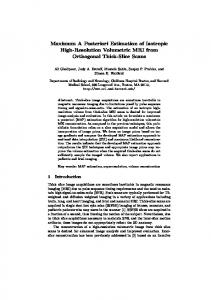
As an example, consider 30 shapes each consisting of six land, , and marks in 2-D X-ray images, then . PCA [1] also known as Karhunen–Loeve transformation [19] and Hotelling transformation [20] is a widely used technique for applications such as dimensionality reduction, data compression, and data visualization [21]. PCA is an orthogonal projection of the data onto a lower dimensional linear subspace, such that the variance of the projected data is maximized sequentially along each new coordinate axis. The linear subspace is not always a precise model of the variability in the data: In the case of shapes, the shapes themselves may intrinsically lie on a nonlinear submanifold. Furthermore, shape normalization using, e.g., Procrustes’ method [22], [23] for neutral position, size, and orientation will also typically project the shapes onto a nonlinear submanifold. As an example, size normalization, such will project the samples onto a dimenas sional hypersphere, as illustrated in Fig. 1 for 2-D data. In this case, PCA may be considered an approximation of the projected variability in the tangent plane under suitable choice of mean. In part, this limitation can be addressed by exploiting the metric of the embedding manifold using techniques, such as, PGA [16]. Nevertheless, we only consider regularized linear models, since our focus is on cases, where the number of samples is small com, and pared to the dimensionality of the embedding space, since we do not assume prior knowledge about any underlying shape manifolds. as PCA models the cloud of (normalized) shapes and covariance a Gaussian distribution with mean . In this paper, we assume that has full rank except for shape normalization, e.g., when normalizing for . The translation, scaling and rotation, then has rank covariance matrix is symmetric and positive semi definite, which is why we may write its eigenvalue decomposition as

Fig. 1. Size normalization of samples (big stars) projects onto a non-Euclidean hypersphere (crosses). A linear model hereof further projects onto a line (circles).

sorted according to for shapes onto a new coordinate system

(4) where is a column vector of ones, such that the is a matrix of , and where outer product the inverse of zero eigenvalues are set to zero. We may consider the shape variations as ordered by variance in an uncorrelated coordinate system, and we may write an approximation of a shape by the absolutely largest eigenvalues as (5) where is column vector in corresponding to the column vector in . The quadratic error of the approximation will be . An often used estimate of the covariance matrix is the ML estimator [24]: The shapes are assumed to be independent and to have identical Gaussian density function, yielding the following joint distribution:

(3) is the column matrix of eigenvectors, where is the diagonal matrix of corand responding eigenvalues. Eigenvectors and values are assumed

. Transforming the as

(6) is the determinant of where called the likelihood of

. This distribution is often , and the point of ML for

1516


varying and is found to be

is derived for completeness in Appendix A and

A Gaussian distribution with mean and covariance on induces a Wishart distribution on the likelihood of [24, Ch. 7]

(7a) (7b) The covariance estimate is slightly biased, but for large the bias is negligible. The speed of the convergence of the estimator is inversely proportional to the number of shapes in a data set. However, faster convergence may be achieved, when prior knowledge is available.

(11) where

is the multivariate Gamma function (12)

The zero mean distribution that best fits the samples as the point of maximum log likelihood for varying

is found as (13)

B. Tikhonov Regularization of Covariance Estimates (ML-T) Regularization is one method for introducing prior knowledge and is often used as a tool for improving the estimate, when the number of samples is small compared to the dimensionality . It is most common to use a of the embedding space, simple form of ridge regression or Tikhonov regularization [4], [7], where nonzero values are added to the diagonal elements of the covariance matrix

identical to (7b). A common prior for covariance matrices is the inverted Wishart to be discussed in the following.

(8)

(14)

. We refer to this method as ML-T. By diagowhere nalizing , it is seen that ML-T only affects the eigenvalues of adding to the eigenvalues of regardless of their value. Adding a constant to zero eigenvalues is useful for regularizing an inversion but may not be for analyzing the subspace , the spanned by the data. It is our experience, that for low absolute eigenvalues require relatively more regularization than the high absolute eigenvalues. Varying as function of absolute eigenvalue is not easily done using ML-T. In this paper, we discuss Bayes estimation of the covariance matrix using the MAP method. We discuss two priors closely tied to the Wishart distribution, which allows for varying degree of regularization depending on absolute eigenvalue. Finally, we discuss a more general Gaussian prior, which allow for prior knowledge on off diagonal interactions. II. MAXIMUM A POSTERIORI COVARIANCE ESTIMATION

A. Inverted Wishart Prior (MAP-IW) A prior giving a simple MAP estimate is the inverted Wishart distribution [24, Ch. 7]

where and are parameters of the distribution. The , inverted Wishart density originates as the distribution of when is Gaussian. Since the evidence is independent on , we find that the point of MAP is (15a)

(15b) using (16) (17)

If we consider a random variable in the space of symmetric, positive semi definite matrices, then Bayes theorem states that

(9) is the posterior, the likelihood, the where is the evidence. We may postulate prior knowlprior, and edge as prior densities and calculate the MAP estimate. As a limiting case, MAP converges to ML as the prior converges to the improper uniform distribution. For all Bayes estimators of covariance matrices presented in this paper, we consider the same likelihood distribution of the sample covariance matrix, (10)

Regarding the structure of (17), we find that it can be similar , , to Tikhonov regularization (8), when and . In any case, the parameter should be set by prior knowledge, e.g., as a measure of the uncertainty in landmark detection by a human operator, or using a geometric distance measure such as (32) also investigated in [25]. We wish to use the inverted Wishart to model independent landmark noise, therefore the structure of the true covariance matrix is assumed to be block diagonal (one block per landmark), and hence must also be block diagonal. Further, we observe that for typical ML estimates of for , the close to zero eigenvalues are particularly poorly estimated. We speculate that this could be caused by overfitting of the first eigenvectors to the data leaving the directions of lesser variance to be underestimated: The first eigenvalue and corresponding eigenvector is


typically estimated through the direction of largest variance in a least squares sense. With only few available samples, this direction of largest variance and the corresponding eigenvalue will, on average, be overestimated. This is straightforward to validate empirically through repeated ML estimation on small samples from a known covariance structure; if the samples afford a direction with variance larger than the known covariance this will always be chosen by the ML estimate. This will, on average, bias the average size of the estimate of the initial eigenvalue. Thus and in contrast to ML-T, we propose to boost small eigenvalues more than large eigenvalues of , by setting to be block-wise proportional to the per landmark inverse ML estimate of its covariance matrix. As an example, for 2-D landmarks distributed as , then (18) is a free mixing parameter. We call this the where MAP-IW. This is not a proper prior, since it depends on the , both measurements. Furthermore, it is noted that when ML-T and MAP-IW enforces full rank. We defer discussion of its usefulness to the experimental section. B. Uncommitted Inverted Wishart Prior (MAP-UIW) The MAP-IW (18) uses an improper prior that depends on an estimate of the covariance of each landmark, which in total may be considered an approximation of . We propose to include directly in the estimation, in which case the maximization results in a system of quadratic equations (19) as derived in Appendix C. This is denoted the MAP-UIW method. As explained above, the MAP-UIW enforces full rank of the estimate. We solve this iteratively using the fix point iteration

(20) where is a sufficiently small constant to avoid divergence. Symmetry of the numerical solution may be guaranteed by taking the average with the transpose, or by only performing calculations for the lower left triangular matrix including the diagonal. We have experimented with both solutions and found no significant differences. For simplicity, we prefer the average. Further, we have experimented with a number of different initial points and the method appears to be robust, however, in . this work we use ML-T as the initial point An alternative solution to (19) is obtained by a different factorization of the (48) (21) this solution theoretically solves the symmetrization issue and employed as a fix point iteration converges with fewer steps than (20). However, there are some numerical drawbacks. First, the need of a SVD decomposition during the square root computation of the matrices slows down the algorithm. Second, since we

1517

perform iterations using a fixed step size, and the space of positive definite matrices (pd) is not a linear vector space, even this elegant solution can in practice step outsize pd-space. Therefore, in our experiments we prefer to use (20). C. Gaussian Prior (MAP-G) An alternative prior is the Gaussian distribution in covariance space (22)

where and represent the mean and variance of the covariance matrix distribution. The variance controls the trade-off between the prior and the ML estimate. A large value of would make the prior uniform and would yield the ML estimate. On the other hand, a very small would yield a delta spike around the mean value and thus bias the estimate heavily towards the mean of the Gaussian. Ideally, the Gaussian prior should be imposed on the space of symmetric, positive definite matrices, e.g., as approximated by the exponential of the norm of the differences of logarithms of matrices [26], but this makes the equation prohibitively complicated, hence we consider (22) a Euclidean approximation. The MAP of (22) is derived in Appendix D and is found to be a system of third degree polynomials (23) We seek its solution by the following iterative scheme:

(24) , when using which we have found to converge for iterative line search in , enforcing symmetry by averaging, . Matrix is a free and using the ML-T as initial point positive semi-definite matrix, which is the embodiment of prior knowledge. Unfortunately, covariance matrices depend on the coordinate system, however, the matrix may be specified in a coordinate system of choice and rotated into the specific coor. dinate system by a suitable rotation matrix as In this section we have considered three different priors to be imposed on our covariance matrix estimates. It is important to bear in mind that the ML-T assumes independence between all elements in the shape, and MAP-IW assume independence between landmarks. Hence both are priors of spatial noise. The MAP-UIW does not have assumption of independence, and MAP-G may be used to directly steer the estimate towards preferred shape variations. Hence both are general priors of shape variations. The classical view of the Inverse Wishart prior has a similar number of parameters as our Gaussian prior. There is, however, a clear difference in how these parameters are used: For the Inverse Wishart prior given , the covariance matrix of maximum probability is the solution to , i.e., the th column in must be perpendicular to the th row in . Hence, if we wish to align the Inverse Wishart prior to favor a particular covariance matrix , then we should select a

1518


from the dimensional manifold fulfilling the above equation, none of which intuitively relate to . Conversely for the Gaussian prior, maximum probability is where , and in order to favor a particular covariance matrix , we simply and intuitively should choose . Furthermore, the additive structure of the Inverse Wishart prior estimators is directly comparable to Tikhonov regularization. In light of the difficulties of large dimensional manifolds described above, we argue that the constrained as well as the uncommitted Wishart priors are the practical extensions of Tikhonov regularization. III. EXPERIMENTAL SETUP We evaluate the performance of the previously described methods for estimating covariance matrices: ML, ML regularized by Tikhonov regularization (ML-T), MAP with an inverted Wishart prior (MAP-IW), MAP with an uncommitted inverted Wishart prior (MAP-UIW), and finally MAP with a Gaussian prior (MAP-G). The evaluation is focused on two main tasks. Firstly, we compare the distance from a known ground-truth covariance matrix to the estimated covariance matrices for synthetic data. Secondly, we evaluate a reconstruction task from low to high-resolution shapes. The details of our validation protocol are described in the following subsections. Section III-A describes the metric used for comparing matrices, Section III-B discusses the reconstruction of high dimensional shape representations, while Section III-C presents the parameter optimization scheme used in the two validation tasks. of the Gaussian Section III-D describes the mean value prior, which we use for our experiments. The results of this validation protocol and the experimental setups are described in Sections IV-A and IV-B, respectively, for synthetic data and for vertebra and cartilage shape reconstruction. A. Matrix Comparison The first part of the validation protocol is a comparison between the ground-truth covariance matrix and different covariance matrix estimates. A matrix norm is required for this purpose. A suitable norm is the Frobenius or two-norm (25) can be the ground truth matrix and a matrix eswhere timated with one of the methods described in this paper. Another useful norm is the log-Euclidean distance between two matrices [26], which approximates the distance between the matrices along the geodesics in the space of symmetric, positive , where definite matrices, , when . With our data, we found no qualitative differences between these norms, and in Section IV-A we present our results using the Frobenius norm. B. Increasing Shape Resolution The direct matrix comparison experiments are not well suited for real data, where ground truth covariance matrices are not available. Therefore, we focus our attention on the example application of increasing shape resolution.

Accurate manual annotation of, e.g., full vertebrae boundaries is tedious and time consuming. Likewise for studies of cartilage shape, more detailed models may lead to more accurate results. These methodologies are described more in detail in Section IV-B. Increasing the shape resolution from a low dimensional manual annotation can be a viable alternative. be an incomplete or lower dimensional shape Letting vector of dimensionality , we would like to find the such that corresponding higher resolution shape (26) is a linear mapping. For our experiments the where matrix is a projection matrix. The lower dimensional shape is aligned to by the standard Procrustes method. Since the system is under-determined, the solution is not uniquely defined. Following Blanz and Vetter [27], we estimate by minimizing the functional (27) Since belongs to the shape model (5), the aforementioned functional transforms to (28) is the parameter vector of the shape model (5), and , where is the eigenvectors and the eigenvalues corresponding to the principal eigenmodes of the covariance matrix. This covariance matrix is estimated using one of the methods described in the previous sections. is a matrix of rank at most . The corresponding reconstruction is [27] where

(29) where , , and sition of , as

are defined by the singular value decompo, and the diagonal matrix is inverted if else

(30)

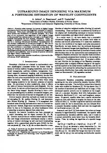
being the th singular value of . By construction, (29) and is invariant to scaling of the underlying regularized covariance matrix with nonzero real constants. C. Parameter Optimization Some of the covariance matrix estimators described in Section II require optimization of parameters such as , , and , and we use cross-validation [28], [29] as follows. For given data, we 20 times randomly select a nonoverlapping train and test set of a specified size. For each pair, we examine a range of parameter values, and for each parameter value, we estimate the generalization error using leave-one-out on the training set. The optimal parameter value is chosen to minimize the generalization error on the training set. The error on the corresponding test set is then calculated using the optimal parameter value. Finally, we report the average performance over all test sets. Fig. 2 shows the 20 different training error


1519

Regardless, considering only points on the surface of an object and for small values of in comparison to the distance between sample points, the Euclidean and the geodesic distances yield similar values of in (32). Further, when objects are flat sheet as is the case for the tibial knee cartilage sheets described in Section IV-B, the Euclidean distance approximates the geodesic distance well. Finally, the Euclidean distance is the easiest to calculate. We choose to model only correlation between nearby points and therefore small values of and Euclidean distance. In this section, we have given an example of the mean value matrix based on the idea that proximity implies covariance. Many other, and perhaps better, choices are possible, but exhaustive investigation is beyond the scope of this paper. IV. EXPERIMENTS Fig. 2. Example of error curves as a function of the MAP-UIW mixing parameter for the range [0; 5]. Each curve is based on a leave-one-out error on a separate set, as described in the main text. On the x-axis the minimum error parameter values are also depicted as stars. For this experiments 10 vertebrae samples were used as a training set.

curves as a function of the mixing parameter for MAP-UIW as well as their detected minima. The same approach is used for optimizing the parameters of the other methods. For the reconstruction evaluation, we note that the parameters of some priors are multiplicative constants and do not require optimization as described previously. D. Mean Value of the Gaussian Prior For the Gaussian prior described in Section II, a crucial aspect is the design of the mean matrix of the prior distribution of in (22) and Section II-C. The design of this matrix must reflect some prior knowledge of the data it represents. For example neighboring points often covary for typical shapes. Therefore, we find it useful to define as a function of the distances between points similarly to [25] (31) where is the th point of the mean of the aligned training examples. Subsequently, we reweigh the distances with an exponential decrease to obtain (32) where is taken element-wise, is the Kronecker product, identity matrix, and is a scale parameter. In and is the , and is of size this way, the resulting matrix is of size . This definition of focuses the regularized estimates to a region of covariance space, where shape point covariances are related by proximity. In [25] geodesic distance were used, but in this work we prefer Euclidean. In general, whether one chooses the Euclidean or the geodesic distance is a modeling choice. If, for example, the shape change is due to friction, then it is fair to assume that shape changes correlate on the surface with nearby points. On the other hand, shape changes for soft tissue may show correlations between surface points that are better modeled by their direct Euclidean distance than their geodesic surface distance.

We now describe the results obtained using the validation protocol and setup described in Section III. First, we report the matrix comparisons between ground truth and covariance estimates for the synthetic data. Secondly, we discuss the shape reconstruction for vertebrae and cartilage shapes. A. Synthetic Shapes, Setup, and Data In this section, we describe the data setup of the experiments with synthetic data and the results of performing a matrix comparison ad described in Section III-A. The synthetic data set is designed to explore two types of variability: linear shape change and independent landmark random variations. First, we design a basis shape resembling a vertebra. Second, the linear shape variation is created by covarying two points along the vertical direction by a normally distributed displacement, which is a typical shape variation seen in real data. Third, normally distributed noise is added to each landmark to simulate annotation noise. We impose three different covariance matrices (33a) (33b) (33c) Fig. 3(a) illustrates the linear shape variation and Fig. 3(b) examples of noise. For the noise, we have used , , , and for the top right and bottom left corners, and for the remaining corners, and for the mid sections. Examples of resulting shapes are shown in Section IV. We estimate the ground truth covariance matrix by using ML on a very large and independent data set of 10.000 samples. Furthermore, we generate 5000 samples, from which the 25 crossfolds are generated as described in Section III-C. The experiments on the synthetic data previously described lead to the results depicted in Figs. 4 and 5. Here, (25) is used to compare the ground truth and the estimated matrices on a small sample size using the different methods (ML, ML-T, MAP-G, MAP-IW, and MAP-UIW) for two noise levels. For each method, the variation for cross-validation is illustrated using standard error of the mean (SEM) error bars. Furthermore, significance of differences between the best method

1520


Fig. 3. (a) Mean shape of the synthetic data and an example of linear shape variations obtained from a Gaussian distribution, where the two central points co-vary vertically. (b) Example of noise variation, where the ellipses denote the standard deviation. Samples of the resulting shapes are shown in Figs. 4 and 5.

and Tikhonov regularization is illustrated by stars, where “*” denotes a t-test p-value below 0.05, “**” below 0.01, and “***” below 0.001. We observe that all the suggested methods outperform ML, and further that the MAP-IW and MAP-UIW priors are suitable choices when the shape variation is dominated by noise (large from (33), illustrated in Fig. 5), while the MAP-G prior is a better choice when there is a dominant shape variation (illustrated in Fig. 4). In addition, Figs. 4 and 5 show that with more available data less regularization is required; and the differences between the methods are less pronounced. It is also important to bear in mind that except for MAP-G, all the methods share the same eigenvectors and differ only in the eigenvalues. This is likely reflected by the clustering of graphs not including MAP-G. B. Increasing Shape Resolution, Setup and Real Data In this section, we explain the experimental setup and results for increasing shape resolution. These experiments are performed on two different data sets: vertebrae and cartilage shapes. For the aim of detecting osteoporotic fragility fractures, the use of high-resolution (full boundary) vertebral shapes may lead to more reliable results than an analysis with low-resolution shapes [30], [31]. For studies on osteoarthritis, more detailed 3D shape models of cartilage may also lead to more accurate results.

Fig. 4. Frobenius norm of the difference between the ground truth covariance matrix and the estimation with ML, ML-T, MAP-IW, MAP-UIW, and MAP-G priors. All the methods are compared for different number of samples, all the parameters are determined by cross-validation as described in Section III-C. : , (b) shows the Subfigure (a) shows the data obtained using (33) with difference as described in Section IV-A, while (c) shows a zoom of the graph in : , and for the cross-validation (b). For the estimation procedure we used ; g, s 2 optimization we investigated the following intervals: m 2 f ; 2 ; : , and ; 2 ; . The stars indicate : ; , statistical significance of the differences between MAP-G and ML-T (Tikhonov) where “*” denotes a t-test p-value below 0.05, “**” below 0.01, and “***” below 0.001.

=01

= 0 25

[0 01 2]

[0 0 1]

[0 5]

1 ... 5

Using the shape reconstruction model (29), a high-resolution shape was reconstructed from a low-dimensional shape. The reconstruction error for a single shape is computed for the points of the boundary as the root mean square error (RMSE) (34)


1521

Fig. 6. (a) An image of a vertebra with the shape annotation. (b) An original (continuous line) and reconstructed (dashed line) shape annotation. The shape’s 52 points are reconstructed using only the six points depicted as the big stars.

Fig. 5. Frobenius norm of the difference between the ground truth covariance matrix and the estimation with ML, ML-T, MAP-IW, MAP-UIW, and MAP-G priors. All the methods are compared for different number of samples, all the parameters are determined by cross-validation as described in Section III-C. Subfigure (a) shows the data obtained using (33) with , (b) shows the difference as described in Section IV-A, while (c) shows a zoom of the graph in (b). For the estimation procedure we used : , and for the cross-val; g, idation optimization we investigated the following intervals: m 2 f ; s 2 : ; ; 2 ; : and ; 2 ; . The stars indicate statistical significance of the differences between MAP-UIW and ML-T (see Fig. 4 for details).

=2

[0 01 2]

[0 0 1]

= 0 25 [0 5]

1 ... 5

The performances of ML, ML-T, MAP-IW, and MAP-UIW over all the test shapes methods are compared using mean for different number of principal eigenmodes. 1) Vertebra Shapes: For general shape analysis, a detailed outline of the shapes are typically used [as illustrated in Fig. 6(a)]. However, for clinical studies on osteoporosis, height ratios are often used for fracture quantification [32], [33] and

only the six vertebra contour points needed to compute these height ratios are routinely marked by expert radiologists. These six landmark points are shown as large stars in Fig. 6(b). The aim is thus to interpolate the full contour [shown as full outline in Fig. 6(b)] from these six points. During the experiments, the shape model is built from the full outline using 52 landmarks and . per shape. Hence, in our experiments We study the vertebra shape variation using images of 75 healthy elderly women, who maintain skeletal integrity over a seven years observation period. The subjects had lateral X-ray of the lumbar spine taken twice, once in 1992–93 (baseline) and again in 2000–01 (follow-up). The used images were digitized using a Vidar DosimetryPro Advantage scanner at 45 m (570 dpi) providing an image resolution of 9651 4008 pixels with 12-bit gray scale. The four lumbar vertebrae L1-L4 were annotated using an annotation tool developed in Matlab. Using both the baseline and follow-up images, we obtain 600 (75 patients visits 4 vertebrae) vertebra shape annotations. To avoid biased results, we only use shapes from the follow-up set. Furthermore, we only use 1 of 4 possible vertebrae per patient selected at random from L1 to L4. Therefore, the total data set of 600 shapes is reduced to 75 shapes. From this we either train on 10 or 20 shapes, and always test on 35 shapes. Fig. 7 shows the mean reconstruction errors for vertebrae shapes obtained using (34) for two different training sample sizes as a function of

1522


Fig. 7. The vertebra reconstruction error for different number of training shapes: (a) 10 and (b) 20. The error measure is described in Section III-B and it is defined in mm. For the estimation procedure we used : , and for the cross-validation optimization we investigated the following intervals: m ,s 2 : ; ; 2 ; : , and ; 2 ; . The stars indicate statistical significance of the differences between MAP-G and ML-T (see Fig. 4 for details).

=1

[0 01 2]

[0 0 1]

= 25 [0 5]

the number of eigenvalues . The experiments demonstrate that all the MAP-based methods improve the reconstruction especially for small sample sizes. Where even these minor improvements in terms of vertebral shape reconstruction can actually affect positively the clinical interpretation in terms of, e.g., establishing first incident vertebral fracture risk [34]. Here, risk evaluation was based on pre-fracture vertebral deformities below established fracture thresholds. Again, the Gaussian prior appears the most suitable for dealing with shapes dominated by global shape variation rather than annotation noise. Fig. 7(a) shows that the ML method has a pronounced error for nine eigenmodes and more caused by the small training set (leave-one-out with only 10 samples). Similarly, the steep rise at 12 eigenvalues in Fig. 7(b) reflects inherent co-linearity of the training set caused by the data set not spanning a subspace larger than 11 eigenvalues. Results not included for 40 training shapes show a similar but less pronounced behavior.

2) Cartilage Shapes: The cartilage data set was composed of 320 knee MRI scans from 80 subjects including both left and right knees and baseline and follow-up scans from a longitudinal 21-month study. In particular, we focus on the tibial cartilage sheets, which are approximately flat. Similarly to the vertebrae, the data set was reduced to 80 samples to ensure only one shape per patient. The MRI acquisition was done on an Esaote C-Scan low field 0.18T clinical scanner using 3D, T1-weighted sequences (flip angle 40 , TR 50 ms, TE 16 ms). The scans were sagittal with slice resolution of 0.7 mm 0.7 mm and slice thickness of 0.8 mm. The dimensions of the scans were 256 256 pixels with around 110 slices. The population includes healthy and diseased knees with varying degree of osteoarthritis from both men and women at ages from 21 to 78. We represent the knee cartilage sheets using the m-rep model [35]. Here, a shape is defined by a spatially regular lattice of medial atoms as depicted in Fig. 8(a). For each knee, we have a three-dimensional m-rep model of the medial tibial cartilage compartment resulting from a fully automatic segmentation [36]. In Fig. 8(a), a cartilage shape model is illustrated for a cropped knee MRI. For m-reps, each atom is representation by a tuple of position, orientation, and radius parameters. A more detailed explanation of this model is given in [37]. For this paper, we only consider the position parameters to allow an analysis similar to the point distribution model used for the vertebra shapes. We evaluate the performance of our method for interpolating medial atoms in order to produce a higher resolution medial model of the cartilage sheets. We perform this evaluation by removing atoms from the models and by measuring how well the interpolation allows for reconstruction of the original model. We train on 10 or 20 shapes, and always test on 35 shapes from the remaining shapes. We produce a low-resolution lattice by removing atoms from the cartilage model, and calculate the mean reconstruction error between the original and the reconstructed 3D shapes using (34). To represent a medial model for a carpoints are used, hence the dimensionality tilage sheet, . During the experiments 24 points are removed leaving . A typfour points, such that the reduced dimensions is ical result of the reconstruction is shown in Fig. 8. The mean reconstruction error using cartilage shapes is obtained using (34) and depicted in Fig. 9. The cartilage shapes show an improvement using the Gaussian prior. Like for the vertebra, the MAP-G method is more appealing because the shapes are dominated more by global shape variations rather than noise. The observation that MAP-G achieves a given reconstruction error using fewer eigenmodes compared to the other methods indicate that MAP-G estimates a more compact representation of the data. V. CONCLUSION Efficient estimation of the covariance matrix is of high importance in statistical shape analysis. Often, the number of available training examples is limited and the estimation of a covariance matrix is a challenging task. We have studied a Bayesian approach to the problem as an alternative to the well-known methods of ML and Tikhonov regularization (ML-T), and we have investigated three different priors: the Inverted Wishart (MAP-IW), the Uncommitted Inverted Wishart (MAP-UIW),


1523

Fig. 9. The cartilage reconstruction error for different number of training shapes: (a) 10 and (b) 20. The error measure is described in Section III-B and it is defined in size normalized shapes. For the estimation procedure we used : , and for the cross-validation optimization we investigated , s 2 : ; ; 2 ; : and the following intervals: m 2 ; . The stars indicate statistical significance of the differ ; ences between MAP-G and ML-T (see Fig. 4 for details).

= 05 [0 5]

Fig. 8. (a) Sagittal and axial MRI slice with the shape model for the medial tibial cartilage compartment. (b) Overlay of the original and the reconstructed cartilage shape viewed axially, (c) coronally, and (d) sagittally. The continuous line is the original shape and the dashed one is the reconstruction. Here the 32 points are reconstructed using only the 4 points depicted as big stars.

and the Gaussian prior (MAP-G). Comparing with respect to the parameters, the ML method has no parameters, the ML-T has one parameter, the MAP-UIW prior has two, while the

= 1

[0 01 2]

[0 0 1]

parameters in their remaining two priors have unconstrained form. Both the MAP-IW prior and the MAP-G prior require a full matrix of parameters, but we have suggested constrained forms, that can be deduced automatically. The MAP-IW method can reflect the noise variation of independent landmark building the matrix as a block diagonal matrix as described in Section II-A. Contrarily, the MAP-G mean matrix allows for inter-landmark interactions, like the suggested geometrical relationships in Section III-D. The Wishart priors also depend on a nuisance parameter , but we remind that for the reconstruction task the results do not seem to be very sensitive to its value. The presented methods perform as well as or better than the ML method especially in the case of small number of training examples. The choice of prior is naturally of great importance for the result. The MAP-IW and MAP-UIW priors assume statistically independent points, and therefore perform better for variations caused by uncorrelated noise. The MAP-G prior is not limited to zero off-block-diagonal elements

1524


and may be used to steer the estimate towards preferred shape variations. Therefore, the choice of prior is related to various factors: the number of samples available, the complexity of the data, the noise variance in the data and the intended application context in which estimated covariance matrices will be used. In general, the prior and specifically for the MAP-G the matrix has to be chosen using prior knowledge optimizing this interplay between prior, data, and application. The focus of this paper has been to introduce novel prior frameworks for covariance matrix estimation and to give simple examples of how they can be used to introduce actual prior knowledge in both artificial and real data sets. But even with the slightly naïve matrix suggested for the MAP-G prior, the improvements over standard approaches are significant for all but one of the examples given. Finally, the paper presented one case with a strong or near-optimal link between prior and data is present. This was the case for the very noisy version of the artificial data, where as the expected the Uncommitted Inverted Wishart prior excelled. In summary, with a sufficient number of samples the standard ML estimation may be the right choice, while for low sample sizes regularization is required. In this case, we argue that our methods can be valid substitutes to Tikhonov regularization.

for , it is posFor minimizing the partial derivatives of sible to isolate the first two terms of (38) considering

(39a) (39b) where a nontrivial solution is

that is (40)

equivalent to (7b). Alternatively, starting from the Wishart likelihood (41) the point of ML for varying

is found to be (42a) (42b) (42c)

APPENDIX A DERIVATION OF MAXIMUM LIKELIHOOD ESTIMATOR For completeness the following gives the derivation of the log-likelihood estimates of the mean vector and covariance matrix using matrix differential calculus [38]. This formulation will be used as a reference point for deriving expressions for the MAP estimates. Using (6), for estimating and from a set of samples, it is possible to seek the maximum point of as (35a)

which implies that (43) or therefore

, also equivalent to (7b).

APPENDIX B DERIVATION OF MAXIMUM A POSTERIORI INVERTED WISHART ESTIMATOR (MAP-IW) In the following, we will derive (17). Starting from (15) and only considering varying , we calculate the differential log as

(35b) For practical reasons it is possible to rewrite the sum under the exponential function of (6) as

(44a)

(36)

(44b)

and to rewrite the logarithm of (6) as (44c) (37) The differential of L, considering only found to be

and

as variables, is

(38)

The MAP using i.i.d. Gaussian likelihood is found to be (45a)

(45b)


which implies that

1525

Notice, that the above equation is also valid for positive semidefinite matrices . Hence, we conclude (46a) (46b)

(51) which is seen to be (19).

and

APPENDIX D DERIVATION OF MAXIMUM A POSTERIORI GAUSSIAN ESTIMATE (MAP-G)

(47)

In the following, we will derive (II-C). Starting from (22) and only considering varying , we find the differential log as

which is seen to be identical to (17). APPENDIX C DERIVATION OF MAXIMUM A POSTERIORI UNCOMMITTED INVERTED WISHART ESTIMATE (MAP-UIW) In the following, we will derive (19). For the moment as. We sume that is invertible, consider (14) and let . Conuse the improper inverted Wishart prior sidering only varying , the differential log of istmi-crimi2131150.xml

(52) (53) The MAP using i.i.d. Gaussian likelihood is found to be (54a)

(54b) which implies that (55a) (48a) (55b) and (48b) (56) (48c)

The equation above can be seen as the third degree matrix polynomial given in (II-C). ACKNOWLEDGMENT

(48d) The MAP using independent and identically distributed (i.i.d.) Gaussian likelihood is found to be

(49a)

(49b) which implies that

(50a) (50b)

The authors would like to acknowledge the Center for Clinical and Basic Research, Ballerup, Denmark, for providing the annotated vertebrae radiographs and the MRI knee scans. The authors would also like to thank the anonymous reviewers for their useful comments. REFERENCES [1] K. Pearson, “On lines and planes of closest fit to systems of points in space,” Philos. Mag., vol. 2, no. 6, pp. 559–572, 1901. [2] L. L. Thurstone, “Multiple factor analysis,” Psychol. Rev., vol. 38, no. 5, pp. 406–427, 1931. [3] C. Stein, “Inadmissibility of the usual estimator for the mean of a multivariate distribution,” in Proc. 3rd Berkeley Symp. Math. Stat. Probabil., 1956, vol. 1, pp. 197–206. [4] A. N. Tikhonov and A. N. Arsenin, Solution of Ill-Posed Problems. Washington: Winston, 1977. [5] B. Efron and C. Morris, “Multivariate empirical Bayes and estimation of covariance matrices,” Ann. Stat., vol. 4, pp. 22–32, 1976. [6] J. H. Friedman, “Regularized discriminant analysis,” J. Am. Stat. Assoc., vol. 84, pp. 165–175, 1989. [7] A. Hoerl and R. W. Kennard, “Ridge regression: Biased estimation for nonorthogonal problems,” Technometrics, vol. 42, no. 1, pp. 80–86, 2000.

1526

[8] L. R. Haff, “Empirical Bayes estimation of the multivariate normal covariance matrix,” Ann. Stat., vol. 8, pp. 586–597, 1980. [9] J. Schaefer and K. Strimmer, “A shrinkage approach to large-scale covariance matrix estimation and implications for functional genomics,” J. Stat. Appl. Genetics Molecular Biol., vol. 4, 2005. [10] W. James and C. Stein, “Estimation with quadratic loss,” in Proc. 4th Berkeley Symp. Math. Stat. Probabil., 1961, vol. 1, pp. 361–379. [11] M. E. Tipping and C. M. Bishop, “Probabilistic principal component analysis,” J. R. Stat. Soc., vol. 21, no. 3, pp. 611–622, 1999. [12] S. Allassonniere, Y. Amit, and A. Trouvé, “Towards a coherent statistical framework for dense deformable template estimation,” J. R. Stat. Soc., vol. 69, no. 1, pp. 3–29, 2007. [13] R. Larsen and K. Hilger, “Statistical shape analysis using non-Euclidean metrics,” Med. Image Anal., vol. 7, no. 4, pp. 417–423, 2003. [14] A. Green, M. Berman, P. Switzer, and M. Craig, “A transformation for ordering multispectral data in terms of image quality with implication for noise removal,” IEEE Trans. Geosci. Remote Sens., vol. 26, no. 1, pp. 65–74, Jan. 1988. [15] P. Switzer, “Min/max autocorrelation factors for multivariate spatial imagery,” Comput. Sci. Stat., vol. 1, pp. 13–16, 1985. [16] P. T. Fletcher, C. Lu, S. M. Pizer, and S. Joshi, “Principal geodesic analysis for the study of nonlinear statistics of shape,” IEEE Trans. Med. Imag., vol. 23, no. 8, pp. 995–1005, Aug. 2004. [17] T. F. Cootes, A. Hill, C. J. Taylor, and J. Haslam, “Use of active shape models for locating structures in medical images,” Image Vis. Comput., vol. 12, pp. 276–285, 1994. [18] D. H. Cooper, T. F. Cootes, C. J. Taylor, and J. Graham, “Active shape models, their training and application,” Computer Vis. Image Understand., vol. 61, pp. 38–59, 1995. [19] K. Karhunen, “Ueber lineare methoden in der wahrscheinlichkeitsrechnung,” Ann. Acad. Sci. Fennicae, vol. 37, pp. 1–79, 1947. [20] H. Hotelling, “Analysis of a complex of statistical variables into principal components,” J. Edu. Psychol., vol. 24, pp. 417–441, 1936. [21] I. T. Jolliffe, Principal Component Analysis. New York: Springer Verlag, 2002, Springer Series Stat.. [22] F. L. Bookstein, “Shape and the information in medical images: A decade of morphometric synthesis,” Comput. Vis. Image Understand., vol. 66, no. 2, pp. 97–118, 1997. [23] C. Goodall, “Procrustes methods in the statistical analysis of shape,” J. R. Stat. Soc., vol. 53, no. 2, pp. 285–339, 1991. [24] T. W. Anderson, An Introduction to Multivariate Statistical Analysis, 3rd ed. New York: Wiley, 2003.


[25] J. Sporring and K. H. Jensen, “Bayes reconstruction of missing teeth,” J. Math. Imag. Vis., vol. 31, pp. 245–254, 2008. [26] P. Fillard, X. Pennec, V. Arsigny, and N. Ayache, “Clinical DT-MRI estimation, smoothing, and fiber tracking with Log-Euclidean metrics,” IEEE Trans. Med. Imag., vol. 26, no. 11, pp. 1472–1482, Nov. 2008. [27] V. Blanz and T. Vetter, Reconstructing the complete 3D shape of faces from partial information Univ. Freiburg, Tech. Rep. Report of Computer Graphics No. 1, 2001. [28] S. Geisser, “Discrimination, allocatory and separatory, linear aspects,” Classification Clustering, pp. 301–330, 1977. [29] P. Lachenbruch, Discriminant Analysis. Royal Oak, MI: Hafner, 1975. [30] M. de Bruijne, M. T. Lund, L. B. Tanko, P. C. Pettersen, and M. Nielsen, “Quantitative vertebral morphometry using neighbor-conditional shape models,” Med. Image Anal., vol. 11, pp. 503–512, 2007. [31] J. Iglesias and M. de Bruijne, “Semi-automatic segmentation of vertebrae in lateral x-rays using a conditional shape model,” Acad. Radiol., pp. 1156–1165, 2007. [32] R. Eastell, S. L. Cedel, H. W. Wahner, B. L. Riggs, and L. J. Melton, “Classification of vertebral fractures,” J. Bone Mineral Res., vol. 4, no. 2, pp. 138–147, 1994. [33] E. V. McCloskey, T. D. Spector, K. S. Eyres, E. D. Fern, N. O’Rourke, S. Vasikaran, and J. A. Kanis, “The assessment of vertebral deformity: A method for use in population studies and clinical trials,” Osteoporos Int., vol. 4, no. 2, pp. 138–147, 1994. [34] M. Lillholm, A. Ghosh, P. Pettersen, M. de Bruijne, E. Dam, M. Karsdal, C. Christiansen, H. K. Genant, and M. Nielsen, “Vertebral fracture risk score for fracture prediction in postmenopausal women,” Osteoporosis Int., 2010. [35] S. Joshi, S. M. Pizer, P. T. Fletcher, A. Thall, and G. Tracton, “Multiscale 3-D deformable model segmentation based on medical description,” Inf. Process. Med. Imag., pp. 64–77, 2001. [36] E. B. Dam, P. T. Fletcher, and S. M. Pizer, “Automatic shape model building based on principal geodesic analysis bootstrapping,” Med. Image Anal., vol. 12, no. 2, pp. 136–151, 2008. [37] P. T. Fletcher, S. Joshi, C. Lu, and S. Pizer, “Gaussian distributions on lie groups and their application to statistical shape analysis,” in Information Processing in Medical Imaging, C. Taylor and J. A. Noble, Eds. : , 2003, pp. 450–462. [38] J. R. Magnus and H. Neudecker, Matrix Differential Calculus with Applications in Statistics and Econometrics, 2nd ed. New York: Wiley, 1999.