MAXIMUM BLOCK IMPROVEMENT AND POLYNOMIAL OPTIMIZATION BILIAN CHEN
∗,
SIMAI HE
†,
ZHENING LI
‡ , AND
SHUZHONG ZHANG
§
Abstract. In this paper we propose an efficient method for solving the spherically constrained homogeneous polynomial optimization problem. The new approach has the following three main ingredients. First, we establish a block coordinate descent type search method for nonlinear optimization, with the novelty being that we only accept a block update that achieves the maximum improvement, hence the name of our new search method: Maximum Block Improvement (MBI). Convergence of the sequence produced by the MBI method to a stationary point is proven. Second, we establish that maximizing a homogeneous polynomial over a sphere is equivalent to its tensor relaxation problem, thus we can maximize a homogeneous polynomial function over a sphere by its tensor relaxation via the MBI approach. Third, we propose a scheme to reach a KKT point of the polynomial optimization, provided that a stationary solution for the relaxed tensor problem is available. Numerical experiments have shown that our new method works very efficiently: for a majority of the test instances that we have experimented with, the method finds the global optimal solution at a low computational cost. Key words. block coordinate descent, polynomial optimization problem, tensor form AMS subject classifications. 90C26, 90C30, 15A69, 49M27
1. Introduction. The optimization models whose objective and constraints are polynomial functions have recently attracted much research attention. This is in part due to an increased demand on the application side (cf. the sample applications in numerical linear algebra [50, 26, 28], material sciences [57], quantum physics [9, 18], and signal processing [16, 4, 53]), and in part due to its own strong theoretical appeal. Indeed, polynomial optimization is a challenging task; at the same time it is rich enough to be fruitful. For instance, even the simplest instances of polynomial optimization, such as maximizing a cubic polynomial over a sphere, is NP-hard (Nesterov [42]). However, the problem is so elementary that it can be even attempted in an undergraduate calculus class. For readers interested in polynomial optimization with simple constraints, we refer to De Klerk [12] for a survey on the computational complexity of optimizing various classes of polynomial functions over a simplex, hypercube or sphere. In particular, De Klerk et al. [13] designed a polynomial-time approximation scheme (PTAS) for minimizing polynomials of fixed degree over the simplex. So far, a few results have been obtained for approximation algorithms with guaranteed worst-case performance ratios for higher degree polynomial optimization problems. Luo and Zhang [39] derived a polynomial-time approximation algorithm to optimize a multivariate quartic polynomial over a region defined by quadratic inequalities. ∗ Department of Systems Engineering and Engineering Management, The Chinese University of Hong Kong, Shatin, Hong Kong (
[email protected]). † Department of Management Sciences, City University of Hong Kong, Kowloon Tong, Hong Kong (
[email protected]). This author’s work is supported in part by Hong Kong GRF Grant CityU143711. ‡ Department of Mathematics, Shanghai University, Baoshan District, Shanghai 200444, China (
[email protected]). This author’s work is supported in part by the Shanghai Leading Academic Discipline Project under Grant S30104. § Industrial and Systems Engineering Program, University of Minnesota, Minneapolis, MN 55455 (
[email protected]). (On leave from Department of Systems Engineering and Engineering Management, The Chinese University of Hong Kong, Shatin, Hong Kong.) This author’s work is supported in part by Hong Kong GRF Grant CUHK419409.
1
2
BILIAN CHEN, SIMAI HE, ZHENING LI, AND SHUZHONG ZHANG
Ling et al. [37] considered the problem of minimizing a biquadratic function over two spheres, and proposed polynomial-time approximation algorithms. He et al. [21] discussed the optimization of homogeneous polynomial functions of any fixed degree over quadratic constraints, and proposed approximation algorithms, with performance ratios improving that of [39, 37]. Recently, So [56] improved the approximation ratio in the case of spherically constrained homogeneous polynomial optimizations. For a general inhomogeneous polynomial optimization over convex compact sets, He et al. [22] proposed polynomial-time approximation algorithms with relative approximation ratios, which is the only result so far with regard to approximation algorithms for an inhomogeneous polynomial. Later, the authors extended their results in [23] by considering polynomials in discrete (typically binary) variables, and designed randomized approximation algorithms. For a recent treatise on the topic, one may refer to the Ph.D. thesis of Li [36]. On the computational side, polynomial optimization problems can be treated as nonlinear programming, and many existing software packages are available, including KNITRO, BARON, MINOS, SNOPT, and Matlab optimization toolbox. (We refer the interested reader to NEOS server [44] for further information.) However, these solvers are not tailor-made for polynomial optimization problems, and so the performance may vary greatly from one problem instance to another. Therefore, it is natural to wonder whether one can design efficient algorithms for specific types of polynomial optimization problems. Prajna et al. [49] presented a package named SOSTOOLS for solving sum of squares polynomial programs, based on the sum of squares (SOS) decomposition for multivariate polynomials, which can be computed using (possibly large size) semidefinite programs. More recently, Henrion et al. [25] developed a specialized tool known as GloptiPoly 3 (its former version GloptiPoly; see Henrion and Lasserre [24]) in finding global optimal solutions for polynomial optimizations based on the SOS approach (see [32, 33, 35, 47, 48] for details). GloptiPoly 3 calls the semidefinite programming (SDP) solver SeDuMi [58]. Therefore, due to the limitation to solve large SDP problems, GloptiPoly 3 may not be the right tool to deal with large size polynomials (say a 6th degree polynomial in 20 variables). However, if the polynomial optimization model in question is sparse in some way, then it is possible to exploit the sparsity in GloptiPoly 3; see [34]. As a matter of fact, SparsePOP [61] makes use of the sparsity explicitly, and is a more appropriate alternative for sparse polynomial optimization based on the SOS approach. Unfortunately, for the problems considered in this paper, the sparsity structure is not readily exploited by SparsePOP. For more information on polynomial optimization, we refer to the recent book of Anjos and Lasserre [2], and the references therein. Spherically constrained homogeneous polynomial optimization models have received some recent research attention, theoretically as well as numerically. One direct approach is to apply the method of Lagrange multipliers to reach a set of multivariate polynomial equations, namely the Karush-Kuhn-Tucker (KKT) system, which provides the necessary conditions for optimality; see, e.g., [16, 28, 65]. In [16], one strives to enumerate all the solutions of a KKT system, not only the global optimum, as all the KKT solutions will be meaningful in this application. Indeed, the authors develop special algorithms for that purpose: e.g., the subdivision methods proposed by Mourrain and Pavone [40], and the generalized normal forms algorithms designed by Mourrain and Tr´ebuchet [41]. However, the shortcomings of these methods are apparent if the degree of the polynomial is high. An important application of spherically constrained homogeneous polynomial optimizations is the best (in the sense of least-
MAXIMUM BLOCK IMPROVEMENT AND POLYNOMIAL OPTIMIZATION
3
square) rank-one approximation of tensors (sometimes also known as the rank-one factorization): find vectors x1 , x2 , · · · , xd for the following minimization problem (Rf ac ) min
∑
(
x1i1 x2i2 · · · xdid − Fi1 i2 ···id
)2
,
i1 ,i2 ,··· ,id
where F = (Fi1 i2 ···id ) is a d-th order tensor. In particular, if the tensor F is supersymmetric (every element Fi1 i2 ···id is invariant under all permutations of (i1 , i2 , · · · , id )), then the optimal vectors x1 , x2 , · · · , xd should coincide (namely they should be equal to each other). The main workhorse for solving the above tensor problem is known as the Alternating Least Square (ALS) method proposed originally by Carroll and Chang [8] and Harshman [19]. However, the ALS method is not guaranteed to converge to a global minimum or a stationary point, only to a solution where the objective function ceases to decrease. There are numerous extensions of the ALS method (e.g., incorporating a line-search procedure in the ALS procedure [46, 55]). Along a related line, De Lathauwer et al. [14] proposed higher-order power method (HOPM) on rank-one approximation of higher-order tensors, which can also be viewed as an extension of the ALS method. Following up on that approach, Kofidis and Regalia [30] devised symmetric higher-order power method (S-HOPM) to rank-one approximation of super-symmetric tensors, and proved its convergence for super-symmetric tensors whenever their corresponding polynomial forms have convexity or concavity. Furthermore, Wang and Qi [62] proposed a greedy method, which iteratively computes the best super-symmetric rank-one approximation of the residual tensors in order to obtain a successive super-symmetric rank-one decomposition. Those methods have nice properties; however they all fail to guarantee convergence for the tensor model (Rf ac ), whether the tensor is super-symmetric or not. For an overview on the recent developments on tensor decomposition, we refer to the excellent survey by Kolda and Bader [31]. Another entirely different but very interesting approach, known as the Z-eigenvalue method, was proposed by Qi et al. [54]. This heuristic cross-hill Z-eigenvalue method aims to solve homogeneous polynomial functions with degree at most three. Motivated by the Block Coordinate Descent (BCD) method for non-differentiable minimization proposed by Tseng [60], and the Iterative Waterfilling Algorithm (IWA) for multiuser power control in digital subscriber lines by Luo and Pang [38], in this paper we shall propose a different method, to be called the Maximum Block Improvement (MBI), for solving spherically constrained homogeneous polynomial optimization problems. Our new method, MBI, guarantees convergence to a stationary point of the problem, which is typically also global optimal in our numerical experiences. The method actually has a general appeal: it can be applied to solve any optimization model with separate block constraints. The proposed MBI approach can naturally be regarded as a local improvement scheme for polynomial optimization, to start from any good initial solutions. Therefore, the new MBI method can be used in combination with any approximation algorithms (such as Khot and Naor [29] and He et al. [21, 22, 23]), to achieve excellent performance in practice while enjoying the theoretical worst case performance guarantees. The remainder of the paper is organized as follows. In Section 2, we introduce the notations and the models to be discussed throughout the paper. Then in Section 3, the general scheme of Maximum Block Improvement method will be introduced, and convergence properties will be discussed in the same section. In Section 4, we present an equivalence result between the spherically constrained homogeneous polynomial
4
BILIAN CHEN, SIMAI HE, ZHENING LI, AND SHUZHONG ZHANG
optimization and its tensor relaxation problem. This will enable the application of the MBI method to solve the polynomial optimization model. Finally, we present the results of our numerical experiments in Section 5. 2. Notations and Models. Let us consider the following multilinear tensor function ∑ F (x1 , x2 , · · · , xd ) = Fi1 i2 ···id x1i1 x2i2 · · · xdid , (2.1) 1≤i1 ≤n1 ,1≤i2 ≤n2 ,··· ,1≤id ≤nd
where xk ∈ ℜnk for k = 1, 2, . . . , d, and F = (Fi1 i2 ···id ) ∈ ℜn1 ×n2 ×···×nd is a d-th order tensor with F being its associated multilinear function. Closely related to the tensor form F is a general d-th degree homogeneous polynomial function f (x), where x ∈ ℜn , with its associated tensor F being super-symmetric. In fact, super-symmetric tensors are bijectively related to homogeneous polynomials; see [31]. Denote F to be the multilinear function defined by the super-symmetric tensor form F, we then have f (x) = F (x, x, · · · , x). | {z }
(2.2)
d
A generic multivariate (inhomogeneous) polynomial function of degree d, denoted by p(x), can be explicitly written as a summation of homogeneous polynomial functions in decreasing degrees, namely p(x) :=
d ∑
fi (x) + f0 =
i=1
d ∑ i=1
Fi (x, x, · · · , x) + f0 , | {z }
(2.3)
i
where x ∈ ℜ , f0 ∈ ℜ, and fi (x) = Fi (x, x, · · · , x) is a homogeneous polynomial | {z } n
i
function of degree i for i = 1, 2, ..., d. Throughout this paper, we use F to denote a multilinear function defined by a tensor form F, f for a homogeneous polynomial function, and p for an inhomogeneous polynomial function; see functions (2.1), (2.2) and (2.3). To avoid triviality, we also assume that at least one component of the tensor form, F in functions F and f , and Fd in function p is nonzero. Throughout the paper we shall use the 2-norm for vectors, matrices and tensors, which is the usual Euclidean norm, defined as √ ∑ ∥F∥ := Fi1 i2 ···id 2 . 1≤i1 ≤n1 ,1≤i2 ≤n2 ,··· ,1≤id ≤nd
The symbol ‘⊗’ represents the vector outer product. For example, for vectors x ∈ ℜn1 , y ∈ ℜn2 , z ∈ ℜn3 , the notion x⊗y⊗z defines a third order tensor F ∈ ℜn1 ×n2 ×n3 , whose (i, j, k)-th element Fijk is equal to xi yj zk . In this paper we shall focus on the polynomial optimization models as considered in He et al. [21, 22], such as optimization of multilinear tensor function (2.1), homogeneous polynomial (2.2) and general inhomogeneous polynomial (2.3) over quadratic constraints, including spherical constraint or the Euclidean ball constraint as a special case. In particular, the authors considered a general model where an inhomogeneous polynomial function is maximized over the intersection of co-centered ellipsoids: (Q)
max s.t.
p(x) xT Qj x ≤ 1, j = 1, 2, ..., m, x ∈ ℜn ,
MAXIMUM BLOCK IMPROVEMENT AND POLYNOMIAL OPTIMIZATION
5
∑m where matrices Qj ≽ 0 for j = 1, 2, ..., m, and j=1 Qj ≻ 0. In this paper we shall pay special attention to the following model (H) max s.t.
f (x) ∥x∥ = 1, x ∈ ℜn .
As we shall see later, (H) has applications in magnetic resonance imaging (MRI), the best rank-one approximation of the super-symmetric tensor F, and the problem of finding the largest eigenvalue of the tensor F; see e.g., [16, 30, 50, 52]. The multilinear tensor relaxation of (H) is (T )
max F (x1 , x2 , · · · , xd ) s.t. ∥xi ∥ = 1, xi ∈ ℜn , i = 1, 2, ..., d.
In He et al. [21], the above relaxation has played a crucial role in the approximation algorithms for solving (H). One of the main contributions of the current paper is to reveal an intrinsic relationship between the optimal solutions of (T ) and (H). Finally, as a matter of notation, for a given optimization problem (P ) we shall denote its optimal value by v(P ). 3. The Maximum Block Improvement (MBI) Method. Towards eventually solving (T ), let us start by considering a generic optimization model in the form of (G) max s.t.
f (x1 , x2 , · · · , xd ) xi ∈ S i ⊆ ℜni , i = 1, 2, ..., d,
where f : ℜn1 +n2 +···+nd → ℜ is a general continuous function, and S i is a general set, i = 1, 2, ..., d. A popular special case of the model is where S i = ℜni , i = 1, 2, ..., d. For that special case, a method known as the Block Coordinate Descent (BCD) is well studied; see Tseng [60] and the references therein. The method calls for maximizing one block, say xi ∈ ℜni , at one time, while all other variables in other blocks are temporarily fixed. One then moves on to alter the choice of the blocks. Very recently, Wright [63] introduced an extension based on BCD. Typically, under various convexity assumptions on the objective function, one is able to show some convergence property of the BCD method (cf. [60]). In fact, the BCD method can be applied regardless of any convexity assumptions, as long as one is able to optimize over one block of variable while fixing the others. A summary of the BCD or other block search methods can be found in Bertsekas [5]. The approach has a relatively long history (sometimes it is also known as the block nonlinear Gauss-Seidel method). Without taking any precaution, the BCD method may not be convergent; see the examples in Powell [51]. In the literature, this issue of convergence has been thoroughly studied. However, the results were not entirely satisfactory. To ensure convergence, one would either require some type of convexity (cf. the discussion in [5]), or the search routine is modified (cf. a proximal-point modification in Grippo and Sciandrone [11]). Our new block search method does not modify the objective function in the block-search subroutine, and at the same time ensures the convergence to a stationary solution within the structure of the BCD framework. The so-called ALS method for tensor decomposition problems (see Section 1) is a special form of the BCD method. We shall remark that the model is reminiscent of a noncooperative game, where S i can be regarded as the strategy set of Player i, i = 1, 2, ..., d. Certainly, in the case of noncooperative game, the objective of each player may be different in general. In a channel spectrum allocation game
6
BILIAN CHEN, SIMAI HE, ZHENING LI, AND SHUZHONG ZHANG
in communication, the corresponding BCD approach is also known as the Iterative Waterfilling Algorithm (IWA); Luo and Pang [38] show that the IWA is convergent to the Nash equilibrium under some fairly loose conditions. It is possible that the IWA may cycle in the absence of these conditions; see an example in [20]. To simplify the analysis, we assume here that S i is compact, i = 1, 2, ..., d. But that alone is insufficient to guarantee the convergence, as we know that even for the special case of the ALS, the iterates may not converge to a stationary point; see e.g., [10, 14, 15, 55]. A sufficient condition for convergence is to take a step that corresponds to the maximum improvement. The enhanced procedure is as follows: Algorithm MBI: The Maximum Block Improvement Method for Solving (G) 0 (Initialization). Choose a feasible solution (x10 , x20 , · · · , xd0 ) with xi0 ∈ S i for i = 1, 2, . . . , d and compute initial objective value v0 := f (x10 , x20 , · · · , xd0 ). Set k := 0. 1 (Block Improvement). For each i = 1, 2, . . . , d, solve (Gi )
i+1 i d max f (x1k , · · · , xi−1 k , x , xk , · · · , xk ) i i s.t. x ∈S ,
and let i+1 i d i := arg max f (x1k , · · · , xi−1 yk+1 k , x , xk , · · · , xk ), i i x ∈S
i+1 i i d wk+1 := f (x1k , · · · , xi−1 k , yk+1 , xk , · · · , xk ). i Let wk+1 := max1≤i≤d wk+1 and i∗ =
2 (Maximum Improvement). i arg max1≤i≤d wk+1 . Let
xik+1 := xik , ∀ i ∈ {1, 2, · · · , d}\{i∗ }, ∗
∗
i xik+1 := yk+1 , vk+1 := wk+1 .
3 (Stopping Criterion). If |vk+1 − vk | < ϵ, stop. Otherwise, set k := k + 1, and go to Step 1. The key assumption in the above process is that problem (Gi ) can be easily solved, which is the case for many applications. For instance, when f (x1 , x2 , · · · , xd ) = −∥F − x1 ⊗ x2 ⊗ · · · ⊗ xd ∥2 , and S i = ℜni , then (Gi ) is simply a least square problem; when f (x1 , x2 , · · · , xd ) is a multilinear tensor form, and S i is convex, then (Gi ) is a convex optimization problem. We shall remark here that a major difference between MBI and IWA (or, for that matter, ALS, BCD or block nonlinear Gauss-Seidel) lies in Step 2: rather than improving among block decision variables alternatively or cyclically, MBI chooses to update the block variables that achieve the maximum improvement. If in Step 2, solving (Gi ) is a least square problem, then MBI becomes a variant of the Alternating Least Square (ALS) method, which is widely used in tensor decompositions (cf. [31]). Unlike the ALS method, as we show next, the MBI method guarantees to converge to a stationary point. Theorem 3.1. If S i is compact for i = 1, 2, ..., d, then any cluster point of the
MAXIMUM BLOCK IMPROVEMENT AND POLYNOMIAL OPTIMIZATION
7
iterates (x1k , x2k , · · · , xdk ), say (x1∗ , x2∗ , · · · , xd∗ ), will be a stationary point for (G); i.e., i i+1 d xi∗ = arg max f (x1∗ , · · · , xi−1 ∗ , x , x∗ , · · · , x∗ ), ∀ i = 1, 2, ..., d. i i x ∈S
Proof. For each fixed (x1 , · · · , xi−1 , xi+1 , · · · , xd ), denote Ri (x1 , · · · , xi−1 , xi+1 , · · · , xd ) to be a best response function to xi , namely Ri (x1 , · · · , xi−1 , xi+1 , · · · , xd ) ∈ arg max f (x1 , · · · , xi−1 , xi , xi+1 , · · · , xd ). i i x ∈S
Suppose that (x1kt , x2kt , · · · , xdkt ) → (x1∗ , x2∗ , · · · , xd∗ ) as t → ∞. Then, for any 1 ≤ i ≤ d, we have i+1 1 i−1 i+1 d d f (x1kt , · · · , xi−1 kt , Ri (x∗ , · · · , x∗ , x∗ , · · · , x∗ ), xkt , · · · , xkt ) i−1 i+1 i+1 1 d d ≤ f (x1kt , · · · , xi−1 kt , Ri (xkt , · · · , xkt , xkt , · · · , xkt ), xkt , · · · , xkt )
≤ f (x1kt +1 , x2kt +1 , · · · , xdkt +1 ) ≤ f (x1kt+1 , x2kt+1 , · · · , xdkt+1 ). By continuity, when t → ∞, it follows that 1 i−1 i+1 d i+1 d 1 2 d f (x1∗ , · · · , xi−1 ∗ , Ri (x∗ , · · · , x∗ , x∗ , · · · , x∗ ), x∗ , · · · , x∗ ) ≤ f (x∗ , x∗ , · · · , x∗ ),
which implies that the above should hold as an equality, since the other inequality is true by the definition of the best response function Ri . Thus, xi∗ is the best response i d i+1 to (x1∗ , · · · , xi−1 ∗ , x∗ , · · · , x∗ ), or equivalently, x∗ is the optimal solution for the problem d max f (x1∗ , · · · , x∗i−1 , xi , xi+1 ∗ , · · · , x∗ ),
xi ∈S i
for all i = 1, 2, ..., d. In many applications, S i is described by inequalities and equalities; e.g., S i = {xi ∈ ℜni | gji (xi ) ≤ 0, j = 1, 2, . . . , mi ; hij (xi ) = 0, j = 1, 2, . . . , ℓi }, where i = 1, 2, ..., d. It is then more convenient to use the so-called KKT conditions, instead of an abstract form of the stationarity, under some constraint qualifications (CQ).1 Corollary 3.2. If S i = {xi ∈ ℜni | gji (xi ) ≤ 0, j = 1, 2, . . . , mi ; hij (xi ) = 0, j = 1, 2, . . . , ℓi } is compact for all i = 1, 2, ..., d, and it satisfies a suitable constraint qualification (cf. footnote 1), then any cluster point of the iterates (x1k , x2k , · · · , xdk ), say (x1∗ , x2∗ , · · · , xd∗ ), will be a KKT point for (G). Proof. As asserted by Theorem 3.1, (x1∗ , x2∗ , · · · , xd∗ ) is a stationary point. Moreover, since a constraint qualification is satisfied for S i , we know that xi∗ is a KKT 1 The most widely used CQs include: the Slater condition; the linear independence constraint qualification (LICQ); the Mangasarian-Fromowitz constraint qualification (MFCQ); the constant rank constraint qualification (CRCQ); the constant positive linear dependence constraint qualification (CPLD); and quasi-normality constraint qualification (QNCQ). For details the reader is referred to a textbook on nonlinear programming; e.g., Bertsekas [5].
8
BILIAN CHEN, SIMAI HE, ZHENING LI, AND SHUZHONG ZHANG
point as well. Namely, there exist uij and vji such that xi = xi∗ satisfies the equations: mi ℓi ∑ ∑ 1 i−1 i i+1 d i i i i ∇ f (x , · · · , x , x , x , · · · , x ) = u ∇g (x ) + vji ∇hij (xi ), ∗ ∗ ∗ ∗ j j x j=1
j=1
uij gji (xi ) = 0, uij ≥ 0, j = 1, 2, . . . , mi , i x ∈ Si, where uij is the Lagrangian multiplier corresponding to the inequality constraint gji (xi ) ≤ 0 for j = 1, 2, ..., mi , and vji is the Lagrangian multiplier corresponding to the equality constraint hij (xi ) = 0 for j = 1, 2, ..., ℓi . Therefore, (x1 , x2 , · · · , xd ) = (x1∗ , x2∗ , · · · , xd∗ ) is a solution for mi ℓi ∑ ∑ ∇xi f (x1 , · · ·, xi−1 , xi , xi+1 , · · ·, xd ) = uij ∇gji (xi ) + vji ∇hij (xi ), i = 1, 2, . . . , d, j=1
j=1
uij gji (xi ) = 0, uij ≥ 0, j = 1, 2, . . . , mi , i = 1, 2, . . . , d, i x ∈ S i , i = 1, 2, . . . , d, which is exactly the KKT system for (G). Therefore, (x1∗ , x2∗ , · · · , xd∗ ) must be a KKT point of (G) as well. Remark that since not all KKT points are stationary, Theorem 3.1 is in fact a stronger statement; however, Corollary 3.2 is convenient to use in many applications. 4. Spherically Constrained Homogeneous Polynomial Optimization. Our study of (G) in this paper is motivated by the tensor optimization model (T ) considered in Section 2: ∑ (T ) max Fi1 i2 ···id x1i1 x2i2 · · · xdid 1≤i1 ≤n1 ,1≤i2 ≤n2 ,··· ,1≤id ≤nd
s.t.
∥xi ∥ = 1, xi ∈ ℜni , i = 1, 2, . . . , d,
which is clearly a special case of (G). Moreover, Algorithm MBI is simple to implement in this case, as optimizing one block while fixing all other blocks is a trivial problem to solve. In fact, simultaneously optimizing over two vectors of variables, while fixing other vectors, are also easy to implement; see [59, 64]. In particular, if d is even, then we may partition the blocks as {x1 , x2 }, · · · , {xd−1 , xd }, and then the subroutine reduces to an eigenvalue problem, rather than least square. (Some numerical results for the latter implementation will be presented in Section 5.) The flexibility in the design of the blocks is an important factor to consider in order for the MBI method to achieve its full efficiency. It is not hard to verify (see e.g., Section 3.4.2 of [36]) that (T ) is actually equivalent to the so-called best rank-one tensor approximation problem given as min s.t.
∥F − λ · x1 ⊗ x2 ⊗ · · · ⊗ xd ∥ λ ∈ ℜ, ∥xi ∥ = 1, xi ∈ ℜni , i = 1, 2, . . . , d.
Traditionally, the ALS method is a popular solution method for such models (see [30, 14]). However, the convergence of the ALS method is not guaranteed in general, as we remarked before, and the new MBI method avoids the pitfalls regarding the convergence.
MAXIMUM BLOCK IMPROVEMENT AND POLYNOMIAL OPTIMIZATION
9
d
In the case when the given d-th order tensor F ∈ ℜn is super-symmetric, then the corresponding super-symmetric rank-one approximation should be
min F − λ · x ⊗ x ⊗ · · · ⊗ x | {z } s.t.
λ ∈ ℜ, x ∈ ℜn .
d
Similar to the non-symmetric case, by imposing the vector x on the unit sphere, we can also verify that the rank-one approximation of super-symmetric tensor problem is indeed equivalent to (H) max
f (x) = F (x, x, · · · , x) | {z } d
∥x∥ = 1, x ∈ ℜn ,
s.t.
where F is the multilinear tensor function defined by the super-symmetric tensor form F. In fact, the above problem (H) is also directly related to computing the maximal eigenvalue of the tensor F; see Qi [50, 52]. The main contribution of this section is to present a new procedure, based on MBI, to effectively compute a KKT point for the best rank-one approximation of a super-symmetric tensor F, namely (H). 4.1. Relationship between (H) and (T ). In He et al. [21], problem (T ) is regarded as a relaxation of (H), and an approximate solution for (T ) is used to construct an approximate solution for (H). Now we shall prove that these two problems are actually equivalent. In fact, we shall prove the following result. d Theorem 4.1. Suppose that F ∈ ℜn is a d-th order super-symmetric tensor with t F being its corresponding multilinear function. Let Gi ∈ ℜm be a t-th order supersymmetric tensor, with Gi being its corresponding multilinear function, i = 1, 2, ..., n. Consider a mapping g : ℜm 7→ ℜn where the i-th component of g is given by gi (x) = Gi (x, x, · · · , x), i = 1, 2, ..., n. If the image set g(ℜm ) ⊆ ℜn is a linear subspace of | {z } t
ℜn , then
max |F (g(x1 ), g(x2 ), · · · , g(xd ))|. max |F (g(x), g(x), · · · , g(x))| = {z } | ∥g(xi )∥=1, i=1,2,...,d
∥g(x)∥=1
d
Proof. Denote the linear subspace g(ℜm ) to be K ⊆ ℜn . It is clear that the two optimization problems in Theorem 4.1 is equivalent to (Hd ) max
|F (y, y, · · · , y )| | {z } d
s.t.
∥y∥ = 1, y ∈ K,
and (Td )
max |F (y 1 , y 2 , · · · , y d )| s.t. ∥y i ∥ = 1, y i ∈ K, i = 1, 2, . . . , d,
respectively. We shall aim to prove that v(Td ) = v(Hd ). The proof is based on the induction on the order of the tensor d. It is trivially true when d = 1. Suppose that v(Td ) = v(Hd ) for d with d ≥ 1. Then, for the case
10
BILIAN CHEN, SIMAI HE, ZHENING LI, AND SHUZHONG ZHANG
d + 1, denote (ˆ y 1 , yˆ2 , · · · , yˆd , yˆd+1 ) to be an optimal solution of (Td+1 ). By induction, we have v(Td+1 ) = =
max
∥y i ∥=1, y i ∈K, i=1,2,...,d
|F (y 1 , y 2 , · · · , y d , yˆd+1 )|
|F (y, y, · · · , y , yˆd+1 )|. | {z } ∥y∥=1, y∈K max
(4.1)
d
Denote S to be the set of all optimal solutions of (Td+1 ) with support 1 or 2, i.e., the number of distinctive vectors of {y 1 , y 2 , · · · , y d , y d+1 } is less than or equal to 2. From (4.1), we know that S is non-empty. By the continuity of F and compactness of the feasible region of y i for i = 1, 2, . . . , d, it is not hard to verify that S is compact. Now consider the following optimization problem: (A)
max
y T z.
(y,y,··· ,y; z,z,··· ,z)∈S
If the optimal value v(A) < 1, then let one of its optimal solution be (ˆ y , yˆ, · · · , yˆ; zˆ, zˆ, · · · , zˆ). Clearly, yˆ ̸= ±ˆ z , because otherwise (ˆ y , yˆ, · · · , yˆ) ∈ S would have v(A) = 1, a contradiction to v(A) < 1. Now denote w ˆ = (ˆ y + zˆ)/∥ˆ y + zˆ∥. Since yˆ, zˆ ∈ K, yˆ ̸= ±ˆ z, and K is a linear subspace of ℜn , we shall have ∥w∥ ˆ = 1 and w ˆ ∈ span(ˆ y , zˆ) ⊂ K. Without loss of generality, we may let F (ˆ y , yˆ, · · · , yˆ; zˆ, zˆ, · · · , zˆ) = v(Td+1 ). (Otherwise use −F instead of F). Since (ˆ y , yˆ, · · · , yˆ; zˆ, zˆ, · · · , zˆ) is an optimal solution for (Td+1 ) and span(ˆ y , zˆ) ⊂ K, it is easy to show that (ˆ y , yˆ, · · · , yˆ; w, ˆ w; ˆ zˆ, zˆ, · · · , zˆ) (namely, replacing the middle (ˆ y , zˆ) by (w, ˆ w)) ˆ is also optimal for (Td+1 ). Apply this replacement procedures until either yˆ or zˆ exhausts, while keeping the optimality for (Td+1 ). Without loss of generality, we may come to an optimal solution in a form of (ˆ y , yˆ, · · · , yˆ; w, ˆ w, ˆ · · · , w) ˆ ∈ S. Let cos θ = v(A) for some θ ∈ (0, π]. Now we shall have w ˆ T yˆ = cos(θ/2) > cos θ = yˆT zˆ = v(A), which contradicts the optimality of (ˆ y , yˆ, · · · , yˆ; zˆ, zˆ, · · · , zˆ) for (A). Thus v(A) must be 1, implying that (A) has a solution with support 1, which proves v(Hd+1 ) = v(Td+1 ). One may be led to the question: are there interesting cases where g(ℜm ) is a subspace? The answer is yes, and the most obvious case is to let t = 1 and g(x) = Gx with G ∈ ℜn×m , and then Theorem 4.1 leads us to: d Corollary 4.2. If F ∈ ℜm is a d-th order super-symmetric tensor with F being its corresponding multilinear function, then max |F (x, x, · · · , x)| = max |F (x1 , x2 , · · · , xd )|. | {z } ∥Gxi ∥=1, i=1,2,...,d
∥Gx∥=1
d
In our particular context, our models (H) and (T ) correspond to G being identity matrix, and m = n. This corollary connects to the so-called “generalized multilinear version of the Cauchy-Bouniakovski-Schwarz inequality” (Hiriart-Urruty [27]), which states that Let F be a super-symmetric multilinear tensor form of order d (≥ 3), and A be a positive semidefinite matrix. If |F (x, x, · · · , x)| ≤ (xT Ax)d/2
∀x ∈ ℜn ,
11
MAXIMUM BLOCK IMPROVEMENT AND POLYNOMIAL OPTIMIZATION
then |F (x1 , x2 , · · · , xd )|2 ≤
d ∏
(xi )T Axi
∀xi ∈ ℜn , i = 1, 2, . . . , d.
i=1
The above inequality was shown by Lojasiewicz (see [6]), and an alternative proof can be found in Nesterov and Nemirovski [43]. Yet, it also follows from Corollary 4.2 by setting A = GT G. Another nontrivial special case when the condition holds is when t = 2, n = 4, m ≥ 3, x ∈ Cm is in the complex-valued domain, and Gi (x, x) is block square-free, i.e., the vector x can be partitioned into two parts, x ˜ and x ˆ, and gi (x) = Gi (x, x) = (˜ xH Gi x ˆ+x ˆH GH x ˜ )/2, i = 1, 2, 3, 4. In that case, Ai, Huang, and Zhang [1] proved i that the joint numerical range g(Cm ) is a convex cone. Due to the block square-free property, it is also not pointed at any direction, hence is a subspace. For our subsequent discussion, the main purpose is to solve (H) via (T ), and so we shall focus on the application of Corollary 4.2. First we remark that the absolute value sign in the objective function of (Td ) can actually be removed, since its optimal value is always nonnegative. Similarly, if d is odd, then the absolute value sign in (Hd ) can also be removed, due to the symmetry of the constraint set; however, for even d, this absolute value sign in (Hd ) is necessary. Ni and Wang [45] proved that Corollary 4.2 holds only for a special case d = 4 and n = 2. We have showed that this property can be extended to a super-symmetric tensor for general dimensions. Interestingly, this result also implies that the best super-symmetric rank-one decomposition of a supersymmetric tensor remains optimal even among all non-symmetric rank-one tensors. Corollary 4.2 establishes the equivalence between (H) and (T ) for odd d, as we discussed before. For an even degree d, one may consider H as the d-th order supersymmetric tensor associated with the homogeneous polynomial h(x) := (xT x)d/2 , and let f (x) := f (x) + τ h(x), where τ = ∥F∥. In that case, f becomes nonnegative on the sphere, and so we can again drop the absolute value sign without affecting the optimal solutions. In both cases, solving (H) can be equivalently transformed into solving (T ), where the MBI method applies. On the other hand, Corollary 4.2 may not hold for other symmetric convex constraints, such as hypercube or simplex; see an example below for the case of a box. Example 4.3. Denote F to be a diagonal matrix Diag (−1, 1), and the boxed constraints are −e ≤ x, y ≤ e with e = (1, 1)T . Then max |F (x, y)| = max | − x1 y1 + x2 y2 | = 2, while max |F (x, x)| = max | − x21 + x22 | = 1. One can further generalize Corollary 4.2 to allow the following mixed homogeneous polynomial function (see e.g., [23, 36]), i.e. f (x1 , x2 , · · · , xs ) := F (x1 , x1 , · · · , x1 , x2 , x2 , · · · , x2 , · · · , xs , xs , · · · , xs ), | {z } | {z } | {z } d1
d2
ds
where xk ∈ ℜnk for k = 1, 2, . . . , s, and the tensor form F ∈ ℜn1 ×n2 ×···×ns has partial symmetric property, namely for any fixed (x2 , x3 , · · · , xs ), F (·, ·, · · · , ·, | {z } d1
d2
ds
d1
x2 , x2 , · · · , x2 , · · · , xs , xs , · · · , xs ) is a super-symmetric d1 -th order tensor form, and | {z } | {z } d2 ds ∑s so on. Denote the order of the tensor F to be d := k=1 ds , then Corollary 4.2
12
BILIAN CHEN, SIMAI HE, ZHENING LI, AND SHUZHONG ZHANG
immediately implies that max s.t.
|f (x1 , x2 , · · · , xs )| = max ∥xi ∥ = 1, i = 1, 2, . . . , s s.t.
|F (y 1 , y 2 , · · · , y d )| ∥y i ∥ = 1, i = 1, 2, . . . , d.
(4.2)
Let us call the left model in the above equation to be (M )
max
∥xi ∥=1, i=1,2,...,s
f (x1 , x2 , · · · , xs ).
Clearly, (M ) is a generalization of the biquadratic model considered in Ling et al. [37] (with s = 2 and d1 = d2 = 2), and the multi-quadratic model considered by So [56] (with d1 = d2 = · · · = ds = 2). Equation (4.2) also suggests a method to solve (M ) by resorting to its multilinear form relaxation (T ), where the MBI method applies. On the other hand, model (M ) can also be solved by directly adopting the MBI method, given that for any fixed (x1 , · · · , xi−1 , xi+1 , · · · , xs ), the maximization over ∥xi ∥ = 1 can be efficiently solved, which in this case is the model (H) with degree di . In particular, we can immediately apply the MBI method to solve the biquadratic model and the multi-quadratic model, since the corresponding subproblem is an eigenvalue problem. We will also test our MBI method in a tri-quadratic case of the model (M ) in the next section. 4.2. Finding a KKT point for (H) using MBI via (T ). Corollary 4.2 suggests a way to solve the homogenous polynomial optimization model (H) by resorting to a seemingly more relaxed tensor optimization model (T ). However, the equivalence is only established at optimality. Nevertheless, one may still search for a KKT solution for (H), by means of searching for a KKT solution for (T ) with identical block variables. (Corollary 4.2 guarantees that such a special KKT point exists, and so the search is valid.) According to our computational experiences, this local search process works very well. In most cases, the KKT solution so-obtained is the true global optimal solution of (H). Let us formalize this search process as follows. We shall work with the version of (T ) and (H) with an absolute sign in the objective function, like in Corollary 4.2. This allows us to swap the direction from x to −x without affecting its objective. As we discussed earlier, adding an absolute sign does not change the problem when d is odd, and also solves (H) when d is even if we modify the objective by adding a (constant) positive term, as we discussed in the previous subsection. Algorithm KKT: Finding a KKT point for (H) 0 Input a KKT solution, say (x10 , x20 , · · · , xd0 ), of (T ) with objective value f0 . Set k := 0 and (r01 , r02 , · · · , r0d ) := (x10 , x20 , · · · , xd0 ). 1 If x1k = ±x2k = · · · = ±xdk , stop. Otherwise, find the closest but not identical pair among these d vectors, i.e., solve max
1≤i fk ; or if fk+1 = (i ∈ {1, 2, · · · , d}\{ik , jk }) such that xi ̸=
13
fk and there is a vector xi
i+1 d F (x1k+1 , · · · , xi−1 k+1 , ·, xk+1 , · · · , xk+1 ) i+1 d ∥F (x1k+1 , · · · , xi−1 k+1 , ·, xk+1 , · · · , xk+1 )∥
;
in either case, starting from (x1k+1 , x2k+1 , · · · , xdk+1 ), apply Algorithm M1 2 d BI to yield a KKT point (rk+1 , rk+1 , · · · , rk+1 ) with a larger objective value for (T ). Otherwise, it is already a KKT point for (T ); set 1 2 d (rk+1 , rk+1 , · · · , rk+1 ) := (x1k+1 , x2k+1 , · · · , xdk+1 ). 4 Let k := k + 1, and go to Step 1. The following property of Algorithm KKT is immediate. Proposition 4.4. For Algorithm KKT, it holds that: 1. Each element in the sequence {(rk1 , rk2 , · · · , rkd )} is a KKT point for (T ). The sequence of the objective values {fk } for (T ) is nondecreasing; 2. If (r∗1 , r∗2 , · · · , r∗d ) is a cluster point of the sequence {(rk1 , rk2 , · · · , rkd )}, then r∗ := r∗1 = ±r∗2 = · · · = ±r∗d . Moreover, (r∗ , r∗ , · · · , r∗ ) or (−r∗ , −r∗ , · · · , −r∗ ) is a KKT point for (T ), and r∗ or −r∗ is a KKT point for (H). 5. Numerical Experiments. In this section, we shall present some preliminary test results for the algorithms proposed in this paper. All the computations are conducted in an Intel(R) Core(TM)2 Quad CPU 2.66GHz computer with 4GB of RAM. The supporting software is Matlab 7.8.0 (R2009a) as a platform. We use Matlab Tensor Toolbox Version 2.4 [3] whenever tensor operations are called, and we use GloptiPoly 3 [25] for general polynomial optimization for the purpose of comparison and set the relaxation order of GloptiPoly 3 by default. To simplify our implementation, we use cvx v1.2 (Grant and Boyd [17]) as a modeling tool for our MBI subroutine. The (termination) precision for these algorithms is set to be 10−6 . For a given maximization problem dimension/structure, we run the algorithms on a number of random instances. GloptiPoly 3 produces an upper bound for the optimal value of that instance, which turns out to be equal to the optimal value in many cases, since the MBI method typically would find a KKT solution equal to the upper bound computed by GloptiPoly 3. We count the percentage of times when this happens in our tests. Moreover, the MBI method is essentially a local improvement, and so it can be started from different initial solutions. Our tests are designed to see the performance of the MBI method over various settings. Below is a list of abbreviations to understand the results summarized in the tables to follow: mean(P): average ratio between solution found by MBI and upper bound by GLP; mean(T): average cpu seconds to solve one instance; mean(I): average number of iterations to solve one instance; mean(T/I): average cpu seconds per iteration; MBI: the maximum block improvement method; dim.: the (d, n) dimension of the test problem; GLP: GloptiPoly 3; # samples: total number of test instances; # starts: number of times to run MBI from random initial solutions (keep the best one); Opt: percentage where the MBI solutions attain the upper bound of GLP.
14
BILIAN CHEN, SIMAI HE, ZHENING LI, AND SHUZHONG ZHANG Table 5.1 Numerical results for (E1 ) when n = 2 and n = 3 dim.
# samples
# starts
GLP
(4, 2)
10
(4, 3)
10
1 2 3 1 2 3 4
mean(T) 1.5961 idem idem 31.6348 idem idem idem
MBI Opt 80% 90% 100% 20% 50% 60% 90%
mean(T) 0.1257 0.1352 0.1472 0.1735 0.2595 0.3113 0.3466
mean(P) 90.83% 94.62% 100% 84.03% 92.67% 93.52% 98.97%
5.1. Randomly Simulated Data. Throughout this subsection, all the data for testing problems are generated in the following manner. First, a d-th order tensor F ′ is randomly generated, with its nd entries following i.i.d. normal distribution, we then symmetrize F ′ to form a super-symmetric tensor F. For co-centered ellipsoidal constraints, we generate n × n matrix Q′j (j = 1, 2, . . . , m), whose entries follow i.i.d. normal distribution, and then let Qj = (Q′j )T Q′j . For comparison, we call GloptiPoly 3 to get optimal value and optimal solution if possible, or else we get an upper bound of the optimal value if GloptiPoly 3 fails to solve the given problem instance. 5.1.1. Multilinear Tensor Function over Spherical Constraints. In this part, we present some numerical tests on (T ). In particular, we consider (E1 )
max s.t.
∑ F (x, y, z, w) = 1≤i,j,k,l≤n Fijkl xi yj zk wl ∥x∥ = ∥y∥ = ∥z∥ = ∥w∥ = 1, x, y, z, w ∈ ℜn ,
where tensor F is super-symmetric. The starting points (x0 , y0 , z0 , w0 ) for Algorithm MBI in our numerical experiments are all randomly generated. In our tests, we consider all the variables in the same constraint set, and dimensions are set to be n = 2 or n = 3. Here the total dimension of the test problems is chosen to be low since for our comparison we need to use GloptiPoly 3 which only works for low dimensions. The comparison is listed in Table 5.1 for (E1 ). Evidently, the results show that Algorithm MBI finds good quality solutions very quickly. The more starts we used to run the MBI algorithm, the higher chance we get an optimal solution. In some cases, GloptiPoly 3 is only capable of providing an upper bound; however our MBI solution achieves these upper bound, proving the optimality of both the GloptiPoly 3 bound and the MBI solution. Besides, a majority of our simulation results show that the KKT point (x∗ , y ∗ , z ∗ , w∗ ) of (E1 ) is automatically a KKT point for the homogeneous polynomial case, namely their block variables are identical already. 5.1.2. Tests of Another Implementation of MBI. Algorithm MBI is optimizing one block while fixing all other blocks. As mentioned in Section 4, simultaneously optimizing over two blocks of variables while fixing other blocks works under the MBI framework as well. Indeed, the similar procedures of Algorithm MBI still perform efficiently, and also the convergence is guaranteed. For convenience, we call this modified procedures MBI′ . In this part, we test the performance of our methods
15
MAXIMUM BLOCK IMPROVEMENT AND POLYNOMIAL OPTIMIZATION Table 5.2 Numerical results for (E2 ) when n = 5, 10, 15 dim.
# samples
(6, 5) (6, 10) (6, 15)
10 10 10
MBI′
MBI mean(T) 0.3087 4.7894 75.1913
mean(I) 57.3 86.7 127.3
mean(T/I) 0.0055 0.0551 0.5901
mean(T) 0.1438 1.1106 22.9004
mean(I) 20.4 38.0 68.3
mean(T/I) 0.0077 0.0297 0.3346
Table 5.3 Numerical results for (E2 ) when (d, n) = (6, 10)
MBI MBI′
1 4.3856 4.2235
2 4.6422 4.8136
3 4.8539 4.7079
4 4.6369 4.5767
5 4.6196 4.6906
6 4.2168 4.4538
7 4.5176 4.3806
8 4.6628 4.7177
9 4.5077 4.2873
10 4.3039 4.3228
MBI and MBI′ for (T ), when d = 6: (E2 ) max s.t.
∑ M (x, y, z, w, p, q) = 1≤i,j,k,l,s,t≤n Mijklst xi yj zk wl ps qt ∥x∥ = ∥y∥ = ∥z∥ = ∥w∥ = ∥p∥ = ∥q∥ = 1, x, y, z, w, p, q ∈ ℜn ,
where tensor M is super-symmetric. In our tests, we choose blocks x, y as a group, and blocks z, w as another group, and blocks p, q as the last group, when implementing MBI′ . Algorithms MBI and MBI′ start from the same point (x0 , y0 , z0 , w0 , p0 , q0 ) which are all randomly generated as before. Two test sets are reported for (E2 ). Table 5.2 reports the average computational time, and Table 5.3 reports the average objective value, where (d, n) = (6, 10). In Table 5.3, we test 10 randomly instances, and each entry is the average objective value by running the corresponding algorithm 20 times. Tables 5.2 and 5.3 show that Algorithm MBI′ is comparable to Algorithm MBI in terms of the solution quality produced; however, Algorithm MBI′ requires much less computational effort on average. This means that the MBI approach is quite flexible and various innovative implementations are possible, and should in fact be encouraged. 5.1.3. General Polynomial Function over Quadratic Constraints. In this part, we report numerical tests on (Q) when d = 4: (E3 ) max p(x) = F4 (x, x, x, x) + F3 (x, x, x) + F2 (x, x) + F1 (x) s.t. xT Qj x ≤ 1, j = 1, 2, ..., m, x ∈ ℜn , 4
3
2
where tensors F4 ∈ ℜn , F3 ∈ ℜn , F2 ∈ ℜn and F1 ∈ ℜn are super-symmetric, and Qj ≽ 0 for j = 1, 2, . . . , m. One natural way to handle an inhomogeneous polynomial function p(x) is through homogenization, e.g., the technique used in [22]. To be specific, by introducing an auxiliary new variable xh , which is set to be 1, we can homogenize function p(x) as (( ) ( ) ( ) ( )) x x x x p(x) = F , , , := F (¯ x, x ¯, x ¯, x ¯) = f (¯ x), xh xh xh xh where f (¯ x) is an (n + 1)-dimensional homogeneous polynomial function of degree 4, 4 and its associated 4-th order super-symmetric tensor form F ∈ ℜ(n+1) . Therefore,
16
BILIAN CHEN, SIMAI HE, ZHENING LI, AND SHUZHONG ZHANG Table 5.4 CPU seconds of GloptiPoly 3 and MBI for (E3 ) when m = 15 n GLP MBI
by denoting x ¯ :=
5 2.1830 24.8763
10 14.6947 42.1047
15 578.3944 42.9723
20 ∞ 43.6567
30 ∞ 44.8106
40 ∞ 44.9569
( ) x , we may equivalently rewrite (E3 ) as 1 (( ) ( ) ( ) ( )) x x x x ¯3 ) max f (¯ (E x) = F , , , 1 1 1 1 s.t. xT Qj x ≤ 1, j = 1, 2, ..., m, x ∈ ℜn .
We shall first call Algorithm MBI to solve the multilinear relaxation problem for ¯3 ), and get a KKT point, to be denoted by (x1∗ , x2∗ , x3∗ , x4∗ ). Then, we select the best (E one from those four vectors as a feasible point for the original model (E3 ), namely, xMBI = arg max1≤i≤4 {p(xi∗ )}. Unlike the equivalence between (H) and (T ) followed ¯3 ) may not be equivalent to its from Corollary 4.2 due to its special structure, (E tensor relaxation problem. Hence, in the last set of tests, starting from the point xMBI , we further apply a projected gradient method [7] (denoted by ‘PGM’ in the table below) to improve the solution of (E3 ). For an overview of gradient projection methods, one is referred to [5]. This method is also used as a supplement in [62, 54] for handling homogeneous polynomial optimization over ball constraint or spherical constraint. The reason to apply the projected gradient method is that this method converges to a KKT point of the problem concerned, and also the optimal projection from ℜn onto the ellipsoidal constraints set E = {x ∈ ℜn | xT Qj x ≤ 1, j = 1, 2, ..., m} can be formulated as an SOCP problem min s.t.
∥x − y∥ x ∈ E,
where y ∈ ℜn is given, which we call cvx to solve under the same computational platform. The starting points for MBI are all randomly generated as before. Two test sets are constructed for (E3 ). First, we fix m = 15 for varying n, and we test the performance of GloptiPoly 3 and MBI in terms of the computational time, regardless of the quality of xMBI obtained by running MBI once (recall the relaxation order of GloptiPoly 3 is set by default). Numerical results are listed in Table 5.4. Each entry is the average time of 10 randomly generated instances. From Table 5.4, we conclude that the computational time of MBI is insensitive to the dimension n, while GloptiPoly 3 is very sensitive to the dimension. In fact, the computational time of MBI is much less than that of GloptiPoly 3 when the dimension n gets large. Second, we fix m = 10 and pick some lower dimensions n, whose problems can be efficiently solved by GloptiPoly 3. We then test the performance of MBI. Specifically, we solve (E3 ) by three different approaches: (1) directly using GloptiPloy 3; (2) applying MBI with randomly generated starting points to get the point xMBI ; (3) using projected gradient method with the starting point xMBI . Numerical results are summarized in Table 5.5, which show the excellent performance of the MBI method. GloptiPoly 3 is a powerful tool for solving (E3 ) with low dimensions. However, the MBI method works very well for polynomial optimization over ellipsoidal constraints even in large dimensions.
MAXIMUM BLOCK IMPROVEMENT AND POLYNOMIAL OPTIMIZATION
17
Table 5.5 Numerical results for (E3 ) when m = 10 dim.
# samples
GLP
20 20 20
mean(T) 1.79 13.01 66.73
(4, 5) (4, 10) (4, 12)
MBI Opt 20% 0% 0%
mean(T) 22.81 38.95 41.36
MBI+PGM mean(P) 85.57% 85.79% 89.61%
Opt 95% 95% 100%
mean(T) 29.68 48.66 50.13
mean(P) 98.21% 99.93% 100%
5.2. Applications. In this subsection, we shall test our proposed algorithms by using data from real applications, including rank-one approximation of supersymmetric tensors, and magnetic resonance imaging (MRI). 5.2.1. Rank-One Approximation of Super-Symmetric Tensors. As discussed in Section 4, homogeneous polynomial optimization over spherical constraint is equivalent to the best rank-one approximation of super-symmetric tensors, hence solvable by our methods. We consider an example in this subsection from Kofidis and Regalia (Example 1 of [30]). The authors of [30] used this example to show that their proposed method S-HOPM did not converge for the particular super-symmetric tensor G ∈ ℜ3×3×3×3 with entries G1111 G1123 G1233 G2233
= 0.2883, = −0.2939, = 0.0919, = 0.2127,
G1112 G1133 G1333 G2333
= −0.0031, = 0.3847, = −0.3619, = 0.2727,
G1113 G1222 G2222 G3333
= 0.1973, G1122 = −0.2485, = 0.2972, G1223 = 0.1862, = 0.1241, G2223 = −0.3420, = −0.3054.
We will test this example using MBI. In our setting, the best rank-one approximation of the tensor G is formulated as ∑ Gijkl xi xj xk xl (E4 ) max 1≤i,j,k,l≤3
s.t.
∥x∥ = 1, x ∈ ℜ3 .
Since the order of G is even, we choose η = 6, and construct a modified and equivalent optimization problem of (E4 ) ∑ (G + ηH)ijkl xi xj xk xl (E5 ) max 1≤i,j,k,l≤3
s.t.
∥x∥ = 1, x ∈ ℜ3 ,
where H is a 4-th order super-symmetric tensor associated with the homogenous polynomial h(x) = (xT x)2 . For the reformulated problem, we apply Algorithm MBI to the multilinear tensor form relaxation of (E5 ): ∑ (E6 ) max G(x, y, z, w) = (G + ηH)ijkl xi yj zk wl 1≤i,j,k,l≤3
s.t.
∥x∥ = ∥y∥ = ∥z∥ = ∥w∥ = 1, x, y, z, w ∈ ℜ3 .
By using MBI with randomly generated starting points, we get three local maximum solutions for (E6 ). For each local maxima (x, y, z, w) we found, it shares the same directions among these 4 vectors when MBI stops, i.e., x = y = z = w. Hence, it provides a local maxima for the original model (E5 ), which is also a local maxima for (E4 ). In Figure 5.1, the total number of iterations in each round
18
BILIAN CHEN, SIMAI HE, ZHENING LI, AND SHUZHONG ZHANG
of MBI is presented, for each local maxima we have found. Indeed, MBI converges very quickly to a local maxima. The optimal value for (E4 ) is 0.8893 (recall we should subtract 6 in the function G(x, y, z, w)), and the optimal solutions are x∗ = ±(0.6671, 0.2487, −0.7022). Hence, the best rank-one approximation for the super-symmetric tensor G is 0.8893 x∗ ⊗ x∗ ⊗ x∗ ⊗ x∗ . 7
Objective Value G(x,y,z,w)
6 5 4 3 2 1
max G(x,y,z,w)=6.8893 max G(x,y,z,w)=6.8169 max G(x,y,z,w)=6.3633
0 −1
0
10
20
30 Iteration
40
50
60
Fig. 5.1. Convergence results of MBI for (E6 )
5.2.2. Magnetic Resonance Imaging (MRI). Finally, we shall conclude this section by considering one real data set for polynomial optimization in Magnetic Resonance Imaging (MRI). Ghosh et al. [16] formulated a fiber detection problem in diffusion MRI by maximizing a homogeneous polynomial function over spherical constraint. In this particular case, the following polynomial optimization model is considered max s.t.
f (x) ∥x∥ = 1, x ∈ ℜ3 ,
where f (x) is a homogeneous polynomial of even degree d. The problem lives in three dimensions as in the real world, and all its local maxima have physical meanings for MRI. We shall test our Algorithm MBI, by using a set of data provided by A. Ghosh and R. Deriche. The corresponding objective function f (x) is 0.74694 − 0.29883 + 0.714359 + 0.316264
x0 4 x0 2 x1 x2 x0 x1 x2 2 x1 2 x2 2
− + − −
0.435103 1.24733 0.397391 0.405544
x0 3 x1 x0 2 x2 2 x0 x2 3 x1 x2 3
+ 0.37089 + 0.0657818 + + 0.794869
x0 3 x2 + 0.454945 x0 2 x1 2 x0 x1 3 − 0.795157 x0 x1 2 x2 x1 4 + 0.139751 x1 3 x2 x2 4 ,
where x = (x0 , x1 , x2 )T . By choosing η = 2, we adopt the same procedures for rankone approximation of super-symmetric tensors discussed in Section 5.2.1 to solve the
MAXIMUM BLOCK IMPROVEMENT AND POLYNOMIAL OPTIMIZATION
19
Table 5.6 Numerical results for MRI Method MBI
GLP
KKT solution ±(0.0116, 0.9992, 0.0382) ±(0.3166, 0.2130, −0.9243) ±(0.9542, −0.1434, 0.2624) ±(0.0116, 0.9992, 0.0382)
Objective value 1.0031 0.9213 0.8428 1.0031
MRI problem. GloptiPoly 3 is also called for comparison. The numerical results are reported in Table 5.6. MBI is able to find all the three local maxima, while GloptiPoly 3 finds only the global maximum. Acknowledgments. We would like to thank A. Ghosh and R. Deriche for providing us a set of real data from the Magnetic Resonance Imaging application. REFERENCES [1] W. Ai, Y. Huang, and S. Zhang, New results on hermitian matrix rank-one decomposition. Mathematical Programming, Series A, 128 (2011), pp. 253–283. [2] M. F. Anjos and J. B. Lasserre, Handbook of Semidefinite, Conic and Polynomial Optimization, Springer, New York, 2011. [3] B. W. Bader and T. G. Kolda, Matlab Tensor Toolbox Version 2.4, http://csmr.ca.sandia.gov/~tgkolda/TensorToolbox, 2010. [4] A. Barmpoutis, B. Jian, B. C. Vemuri, and T. M. Shepherd, Symmetric positive 4th order tensors & their estimation from diffusion weighted MRI, in N. Karssemijer and B. Lelieveldt ed., LNCS 4584 (2007), pp. 308–319. [5] D. P. Bertsekas, Nonlinear Programming, second edition, Athena Scientific, Belmont, 1999. [6] J. Bochnak and J. Siciak, Polynomials and multilinear mappings in topological vector spaces, Studia Math., 39 (1971), pp. 59–76. [7] P. H. Calamai and J. J. Mor´ e, Projected gradient methods for linearly constrained problems. Mathematical Programming, 39 (1987), pp. 93–116. [8] J. D. Carroll and J. J. Chang, Analysis of individual differences in multidimensional scaling via an N-way generalization of “Eckart-Young” decomposition, Psychometrika, 35 (1970), pp. 283–319. [9] G. Dahl, J. M. Leinaas, J. Myrheim, and E. Ovrum, A tensor product matrix approximation problem in quantum physics, Linear Algebra and Its Applications, 420 (2007), pp. 711–725. [10] E. F. Gonzalez and Y. Zhang, Accelerating the Lee-Seung algorithm for nonnegative matrix factorization, preprint, March 2005. [11] L. Grippo and M. Sciandrone, On the convergence of the block nonlinear Gauss-Seidel method under convex constraints, Operations Research Letters, 26 (2000), pp. 127–136. [12] E. de Klerk, The complexity of optimizing over a simplex, hypercube or sphere: a short survey, Central European Journal of Operations Research, 16 (2008), pp. 111–125. [13] E. de Klerk, M. Laurent, and P. A. Parrilo, A PTAS for the minimization of polynomials of fixed degree over the simplex, Theoretical Computer Science, 261 (2006), pp. 210–225. [14] L. De Lathauwer, B. De Moor, and J. Vandewalle, On the best rank-1 and rank(R1 , R2 , · · · , RN ) approximation of higher-order tensors, SIAM Journal on Matrix Analysis and Applications, 21 (2000), pp. 1324–1342. [15] L. De Lathauwer, and D. Nion, Decompositions of a higher-order tensor in block terms—Part III: Alternating least squares algorithms, SIAM Journal on Matrix Analysis and Applications, 30 (2008), pp. 1067–1083. [16] A. Ghosh, E. Tsigaridas, M. Descoteaux, P. Comon, B. Mourrain, and R. Deriche, A polynomial based approach to extract the maxima of an antipodally symmetric spherical function and its application to extract fiber directions from the orientation distribution function in diffusion MRI, Computational Diffusion MRI Workshop (CDMRI’08), New York, 2008. [17] M. Grant and S. Boyd, CVX: Matlab Software for Disciplined Convex Programming, version 1.2, http://cvxr.com/cvx, 2010. [18] L. Gurvits, Classical deterministic complexity of Edmonds’ problem and quantum entangle-
20
[19]
[20] [21] [22]
[23]
[24] [25] [26] [27]
[28] [29] [30] [31] [32] [33] [34] [35] [36] [37] [38]
[39]
[40] [41]
[42] [43] [44] [45]
BILIAN CHEN, SIMAI HE, ZHENING LI, AND SHUZHONG ZHANG ment, Proceedings of the Thirty-Fifth ACM Symposium on Theory of Computing, 10–19, ACM, New York, 2003. R. A. Harshman, Foundations of the PARAFAC procedure: Models and conditions for an “explanatory” multi-modal factor analysis, UCLA Working Papers in Phonetics, 16, 1–84, http://publish.uwo.ca/~harshman/wpppfac0.pdf, 1970. S. He, M. Li, S. Zhang and Z.-Q. Luo, A nonconvergent example for the iterative water-filling algorithm, Numerical Algebra, Control and Optimization, 1 (2011), pp. 147–150. S. He, Z. Li, S. Zhang, Approximation algorithms for homogeneous polynomial optimization with quadratic constraints, Mathematical Programming, Series B, 125 (2010), pp. 353–383. S. He, Z. Li, and S. Zhang, General constrained polynomial optimization: an approximation approach, Technical Report SEEM2009-06, Department of Systems Engineering and Engineering Management, The Chinese University of Hong Kong, 2009. S. He, Z. Li, and S. Zhang, Approximation algorithms for discrete polynomial optimization, Technical Report SEEM2010-01, Department of Systems Engineering and Engineering Management, The Chinese University of Hong Kong, 2010. D. Henrion and J. B. Lasserre, GloptiPoly: Global optimization over polynomials with Matlab and SeDuMi, ACM Tran. Math. Soft., 29 (2003), pp. 165–194. D. Henrion, J. B. Lasserre, and J. Loefberg, GloptiPoly 3: Moments, optimization and semidefinite programming, Optimization Methods and Software, 24 (2009), pp. 761–779. C. J. Hillar and L.-H. Lim, Most tensor problems are NP hard, Preprint, http://www.stat.uchicago.edu/~lekheng/work/np.pdf, 2009. J.-B. Hiriart-Urruty, A new series of conjectures and open questions in optimization and matrix analysis, ESAIM: Control, Optimisation and Calculus of Variations, 15 (2009), pp. 454– 470. P. M. J. Hof, C. Scherer and P.S.C. Heuberger, Model-Based Control: Bridging Rigorous Theory and Advanced Technology, Part 1, pp. 49–68. Springer–Verlag, Berlin Heidelberg, 2009. S. Khot and A. Naor, Linear equations modulo 2 and the L1 diameter of convex bodies, the 48th Annual IEEE Symposium on Foundations of Computer Science (2007), pp. 318–328. E. Kofidis and P. A. Regalia, On the best rank-1 approximation of higher order supersymmetric tensors, SIAM Journal on Matrix Analysis and Applications, 23 (2002), pp. 863–884. T. G. Kolda and B. W. Bader, Tensor decompositions and applications, SIAM Review, 51 (2009), pp. 455–500. J. B. Lasserre, Global optimization with polynomials and the problem of moments, SIAM Journal on Optimization, 11 (2001), pp. 796–817. J. B. Lasserre, Polynomials nonnegative on a grid and discrete representations, Transactions of the American Mathematical Society, 354 (2001), pp. 631–649. J. B. Lasserre, Convergent SDP relaxations in polynomial optimization with sparsity, SIAM Journal on Optimization, 17 (2006), pp. 822–843. J. B. Lasserre, A sum of squares approximation of nonnegative polynomials, SIAM Review, 49 (2007), pp. 651–669. Z. Li, Polynomial Optimization Problems—Approximation Algorithms and Applications, Ph.D. Thesis, The Chinese Univesrity of Hong Kong, June 2011. C. Ling, J. Nie, L. Qi, and Y. Ye, Biquadratic optimization over unit spheres and semidefinite programming relaxations, SIAM Journal on Optimization, 20 (2009), pp. 1286–1310. Z.-Q. Luo and J.-S. Pang, Analysis of iterative waterfilling algorithm for multiuser power control in digital subscriber lines, EURASIP Journal on Applied Signal Processing, 2006 (2006), pp. 1–10. Z.-Q. Luo and S. Zhang, A semidefinite relaxation scheme for multivariate quartic polynomial optimization with quadratic constraints, SIAM Journal on Optimization, 20 (2010), pp. 1716–1736. B. Mourrain and J. P. Pavone, Subdivision methods for solving polynomial equations, Journal of Symbolic Computation, 44 (2009), pp. 292–306. B. Mourrain and P. Tr´ ebuchet, Generalized normal forms and polynomial system solving. in M. Kauers, ed., Proc. Intern. Symp. on Symbolic and Algebraic Computation (2005), New York, ACM Press, pp. 253–260. Yu. Nesterov, Random walk in a simplex and quadratic optimization over convex polytopes, CORE Discussion Paper, UCL, Louvain-la-Neuve, Belgium, 2003. Yu. Nesterov and A. Nemirovski, Interior-Point Polynomial Algorithms in Convex Programming, SIAM Studies in Applied Mathematics, 1994. Network-Enabled Optimization Systems (NEOS) Server for Optimization, http://www.neos-server.org/neos. G. Ni and Y. Wang, On the best rank-1 approximation to higher-order symmetric tensors,
MAXIMUM BLOCK IMPROVEMENT AND POLYNOMIAL OPTIMIZATION
21
Mathematical and Computer Modelling, 46 (2007), pp. 1345–1352. [46] D. Nion and L. De Lathauwer, An enhanced line search scheme for complex-valued tensor decompositions, Application in DS-CDMA, Signal Processing, 88 (2008), pp. 749–755. [47] P. A. Parrilo, Structured Semidefinite Programs and Semialgebraic Geometry Methods in Robustness and Optimization, Ph.D. Dissertation, California Institute of Technology, CA, 2000. [48] P. A. Parrilo, Semidefinite programming relaxations for semialgebraic problems, Mathematical Programming, Series B, 96 (2003), pp. 293–320. [49] S. Prajna, A. Papachristodoulou, P.A. Parrilo, Introducing SOSTOOLS: a general purpose sum of squares programming solver, Proceedings of the 41st IEEE Conference on Decision and Control, Las Vegas, 2002. [50] L. Qi, Eigenvalues of a real supersymmetric tensor, Journal of Symbolic Computation, 40 (2005), pp. 1302–1324. [51] M. J. D. Powell, On search directions for minimization algorithms, Mathematical Programming, 4 (1973), pp. 193–201. [52] L. Qi, Eigenvalues and invariants of tensors, Journal of Mathematical Analysis and Applications, 325 (2007), pp. 1363–1377. [53] L. Qi and K. L. Teo, Multivariate polynomial minimization and its application in signal processing, Journal of Global Optimization, 26 (2003), pp. 419–433. [54] L. Qi, F. Wang, and Y. Wang, Z-eigenvalue methods for a global polynomial optimization problem, Mathematical Programming, Series A, 118 (2009), pp. 301–316. [55] M. Rajih, P. Comon, and R. A. Harshman, Enhanced line search: A novel method to accelerate PARAFAC, SIAM Journal on Matrix Analysis and Applications, 30 (2008), pp. 1128–1147. [56] A. M.-C. So, Deterministic approximation algorithms for sphere constrained homogeneous polynomial optimization problems, Mathematical Programming, Series B, 129 (2011), pp. 357– 382. [57] S. Soare, J.W. Yoon, and O. Cazacu, On the use of homogeneous polynomials to develop anisotropic yield functions with applications to sheet forming, International Journal of Plasticity, 24 (2008), pp. 915–944. [58] J. F. Sturm, SeDuMi 1.02, a Matlab toolbox for optimization over symmetric cones, Optimization Methods and Software, 11 & 12 (1999), pp. 625–653. [59] J. F. Sturm and S. Zhang, On cones of nonnegative quadratic functions, Mathematics of Operations Research, 28 (2003), pp. 246–267. [60] P. Tseng, Convergence of a block coordinate descent method for nondifferentiable minimization, Journal of Optimizatoin Theory and Applications, 109 (2001), pp. 475–494. [61] H. Waki, S. Kim, M. Kojima, M. Muramatsu, and H. Sugimoto, Algorithm 883: SparsePOP: A sparse semidefinite programming relaxation of polynomial optimization problems, ACM Transactions on Mathematical Software, 35 (2008), pp. 1–13. [62] Y. Wang and L. Qi, On the successive supersymmetric rank-1 decomposition of higher-order supersymmetric tensors, Numerical Linear Algebra with Applications, 14 (2007), pp. 503– 519. [63] S. Wright, Accelerated block-coordinate relaxation for regularized optimization, Working Paper, University of Wisconsin, 2010. [64] Y. Ye and S. Zhang, New results on quadratic minimization, SIAM Journal on Optimization, 14 (2003), pp. 245–267. [65] T. Zhang and G. H. Golub, Rank-one approximation to high order tensors, SIAM Journal on Matrix Analysis and Applications, 23 (2001), pp. 534–550.