maximum entropy flow networks - Department of Statistics - Columbia ...

Under review as a conference paper at ICLR 2017

M AXIMUM E NTROPY F LOW N ETWORKS Gabriel Loaiza-Ganem∗, Yuanjun Gao∗ & John P. Cunningham Department of Statistics Columbia University New York, NY 10027, USA {gl2480,yg2312,jpc2181}@columbia.edu

A BSTRACT Maximum entropy modeling is a flexible and popular framework for formulating statistical models given partial knowledge. In this paper, rather than the traditional method of optimizing over the continuous density directly, we learn a smooth and invertible transformation that maps a simple distribution to the desired maximum entropy distribution. Doing so is nontrivial in that the objective being maximized (entropy) is a function of the density itself. By exploiting recent developments in normalizing flow networks, we cast the maximum entropy problem into a finite-dimensional constrained optimization, and solve the problem by combining stochastic optimization with the augmented Lagrangian method. Simulation results demonstrate the effectiveness of our method, and applications to finance and computer vision show the flexibility and accuracy of using maximum entropy flow networks.

1

I NTRODUCTION

The maximum entropy (ME) principle (Jaynes, 1957) states that subject to some given prior knowledge, typically some given list of moment constraints, the distribution that makes minimal additional assumptions – and is therefore appropriate for a range of applications from hypothesis testing to price forecasting to texture synthesis – is that which has the largest entropy of any distribution obeying those constraints. First introduced in statistical mechanics by Jaynes (1957), and considered both celebrated and controversial, ME has been extensively applied in areas including natural language processing (Berger et al., 1996), ecology (Phillips et al., 2006), finance (Buchen & Kelly, 1996), computer vision (Zhu et al., 1998), and many more. Continuous ME modeling problems typically include certain expectation constraints, and are usually solved by introducing Lagrange multipliers, which under typical assumptions yields an exponential family distribution (also called Gibbs distribution) with natural parameters such that the expectation constraints are obeyed. Unfortunately, fitting ME distributions in even modest dimensions poses significant challenges. First, optimizing the Lagrangian for a Gibbs distribution requires evaluating the normalizing constant, which is in general computationally very costly and error prone. Secondly, in all but the rarest cases, there is no way to draw samples independently and identically from this Gibbs distribution, even if one could derive it. Third, unlike in the discrete case where a number of recent and exciting works have addressed the problem of estimating entropy from discrete-valued data (Jiao et al., 2015; Valiant & Valiant, 2013), estimating differential entropy from data samples remains inefficient and typically biased. These shortcomings are critical and costly, given the common use of ME distributions for generating reference data samples for a null distribution of a test statistic. There is thus ample need for a method that can both solve the ME problem and produce a solution that is easy and fast to sample. In this paper we develop maximum entropy flow networks (MEFN), a stochastic-optimization-based framework and algorithm for fitting continuous maximum entropy models. Two key steps are required. First, conceptually, we replace the idea of maximizing entropy over a density directly with maximizing, over the parameter space of an indexed function family, the entropy of the density induced by mapping a simple distribution (a Gaussian) through that optimized function. Modern ∗

These authors contributed equally.

1

Under review as a conference paper at ICLR 2017

neural networks, particularly in variational inference (Kingma & Welling, 2013; Rezende & Mohamed, 2015), have successfully employed this same idea to generate complex distributions, and we look to similar technologies. Secondly, unlike most other objectives in this network literature, the entropy objective itself requires evaluation of the target density directly, which is unavailable in most traditional architectures. We overcome this potential issue by learning a smooth, invertible transformation that maps a simple distribution to an (approximate) ME distribution. Recent developments in normalizing flows (Rezende & Mohamed, 2015; Dinh et al., 2016) allow us to avoid biased and computationally inefficient estimators of differential entropy (such as the nearest-neighbor class of estimators like that of Kozachenko-Leonenko; see Berrett et al. (2016)). Our approach avoids calculation of normalizing constants by learning a map with an easy-to-compute Jacobian, yielding tractable probability density computation. The resulting transformation also allows us to reliably generate iid samples from the learned ME distribution. We demonstrate MEFN in detail in examples where we can access ground truth, and then we demonstrate further the ability of MEFN networks in equity option prices fitting and texture synthesis. Primary contributions of this work include: (i) addressing the substantial need for methods to sample ME distributions; (ii) introducing ME problems, and the value of including entropy in a range of generative modeling problems, to the deep learning community; (iii) the novel use of constrained optimization for a deep learning application; and (iv) the application of MEFN to option pricing and texture synthesis, where in the latter we show significant increase in the diversity of synthesized textures (over current state of the art) by using MEFN.

2 2.1

BACKGROUND M AXIMUM ENTROPY MODELING AND G IBBS DISTRIBUTION

We consider a continuous random variable Z ∈ Z ⊆ Rd with density p, where p has differential R entropy H(p) = − p(z) log p(z)dz and support supp(p). The goal of ME modeling is to find, and then be able to easily sample from, the maximum entropy distribution given a set of moment and support constraints, namely the solution to: p∗

=

maximize H(p) subject to EZ∼p [T (Z)] = 0 supp(p) = Z,

(1)

where T (z) = (T1 (z), ..., Tm (z)) : Z → Rm is the vector of known (assumed sufficient) statistics, and Z is the given support of the distribution. Under standard regularity conditions, the optimization problem can be solved by Lagrange multipliers, yielding an exponential family p∗ of the form: p∗ (z) ∝ eη

>

T (z)

1(z ∈ Z)

(2)

where η ∈ Rm is the choice of natural parameters of p∗ such that Ep∗ [T (Z)] = 0. Despite this simple form, these distributions are only in rare cases tractable from the standpoint of calculating η, calculating the normalizing constant of p∗ , and sampling from the resulting distribution. There is extensive literature on finding η numerically (Darroch & Ratcliff, 1972; Salakhutdinov et al., 2002; Della Pietra et al., 1997; Dudik et al., 2004; Malouf, 2002; Collins et al., 2002), but doing so requires computing normalizing constants, which poses a challenge even for problems with modest dimensions. Also, even if η is correctly found, it is still not trivial to sample from p∗ . Problemspecific sampling methods (such as importance sampling, MCMC, etc.) have to be designed and used, which is in general challenging (burn-in, mixing time, etc.) and computationally burdensome. 2.2

N ORMALIZING FLOWS

Following Rezende & Mohamed (2015), we define a normalizing flow as the transformation of a probability density through a sequence of invertible mappings. Normalizing flows provide an elegant way of generating a complicated distribution while maintaining tractable density evaluation. Starting with a simple distribution Z0 ∈ Rd ∼ p0 (usually taken to be a standard multivariate 2

Under review as a conference paper at ICLR 2017

Gaussian), and by applying k invertible and smooth functions fi : Rd → Rd (i = 1, ..., k), the resulting variable Zk = fk ◦ fk−1 ◦ · · · ◦ f1 (Z0 ) has density: pk (zk ) = p0 (f1−1 ◦ f2−1 ◦ · · · ◦ fk−1 (zk ))

k Y

| det(Ji (zi−1 ))|−1 ,

(3)

i=1

where Ji is the Jacobian of fi . If the determinant of Ji can be easily computed, pk can be computed efficiently. Rezende & Mohamed (2015) proposed two specific families of transformations for variational inference, namely planar flows and radial flows, respectively: fi (z) = z + ui h(wiT z + bi )

and

fi (z) = z + βi h(αi , ri )(z − z0i ),

(4)

where bi ∈ R, ui , wi ∈ Rd and h is an activation function in the planar case, and where βi ∈ R, αi > 0, z0i ∈ Rd , h(α, r) = 1/(α + r) and ri = ||z − z0i || in the radial. Recently Dinh et al. (2016) proposed a normalizing flow with convolutional, multiscale structure that is suitable for image modeling and has shown promise in density estimation for natural images.

3 3.1

M AXIMUM ENTROPY FLOW NETWORK (MEFN) ALGORITHM F ORMULATION

Instead of solving Equation 2, we propose solving Equation 1 directly by optimizing a transformation that maps a random variable Z0 , with simple distribution p0 , to the ME distribution. Given a parametric family of normalizing flows F = {fφ , φ ∈ Rq }, we denote pφ (z) = p0 (fφ−1 (z))| det(Jφ (z))|−1 as the distribution of the variable fφ (Z0 ), where Jφ is the Jacobian of fφ . We then rewrite the ME problem as: φ∗

= maximize H(pφ ) subject to EZ0 ∼p0 [T (fφ (Z0 ))] = 0 supp(pφ ) = Z.

(5)

When p0 is continuous and F is suitably general, the program in Equation 5 recovers the ME distribution pφ exactly. With a flexible transformation family, the ME distribution can be well approximated. In experiments we found that taking p0 to be a standard multivariate normal distribution achieves good empirical performance. Taking p0 to be a bounded distribution (e.g. uniform distribution) is problematic for learning transformations near the boundary, and heavy tailed distributions (e.g. Cauchy distribution) caused similar trouble due to large numbers of outliers. 3.2

A LGORITHM

We solved Equation 5 using the augmented Lagrangian method. Denote T (φ) = E(T (fφ (Z0 ))), the augmented Lagrangian method uses the following objective: c L(φ; λ, c) = −H(pφ ) + λ> T (φ) + ||T (φ)||2 2

(6)

where λ ∈ Rm is the Lagrange multiplier and c > 0 is the penalty coefficient. We minimize Equation 6 for a non-decreasing sequence of c and well-chosen λ. As a technical note, the augmented Lagrangian method is guaranteed to converge under some regularity conditions (Bertsekas, 2014). As is usual in neural networks, a proof of these conditions is challenging and not yet available, though intuitive arguments suggest that most of them should hold. We omit a more thorough discussion about them and rely instead on the empirical results of the algorithm to claim that it is indeed solving the optimization problem. For a fixed (λ, c) pair, we optimize L with stochastic gradient descent. Owing to our choice of network and the resulting ability to efficiently calculate the density pφ (z(i) ) for any sample point 3

Under review as a conference paper at ICLR 2017

Algorithm 1 Training the MEFN 1: initialize φ = φ0 , set c0 > 0 and λ0 . 2: for Augmented Lagrangian iteration k = 1, ..., kmax do 3: for SGD iteration i = 1, ..., imax do (i) 4: Sample z(1) , ..., z(n) ∼ p0 , get transformed variables zφ = fφ (z(i) ), i = 1, ..., n 5: Update φ by descending its stochastic gradient (using e.g. ADADELTA (Zeiler, 2012)): n

∇φ L(φ; λk , ck ) ≈

n n 2 X 2 1 X 2 X (i) (i) (i) > 1 ∇φ T (zφ ) · ∇φ log pφ (zφ ) + λk ∇φ T (zφ ) + ck n i=1 n i=1 n i=1 n

n X

(i)

T (zφ )

i= n +1 2

end for (i) Sample z(1) , ..., z(˜n) ∼ p0 , get transformed variables zφ = fφ (z(i) ), i = 1, ..., n ˜ Pn˜ (i) 1 8: Update λk+1 = λk + ck n˜ i=1 T (zφ ) 9: Update ck+1 ≥ ck (see text for detail) 10: end for 6: 7:

z(i) (which are easy-to-sample iid draws from the multivariate normal p0 ), we compute the unbiased estimator of H(pφ ) with: n 1X log pφ (fφ (z(i) )) (7) H(pφ ) ≈ − n i=1 T (φ) can also be estimated without bias by taking a sample average of z(i) draws. The resulting optimization procedure is detailed in Algorithm 1, of which step 9 requires some detail: denoting φk as the resulting φ after imax SGD iterations at the augmented Lagrangian iteration k, the usual update rule for c (Bertsekas, 2014) is:  βck , if ||T (φk+1 )|| > γ||T (φk )|| ck+1 = (8) ck , otherwise where γ ∈ (0, 1) and β > 1. Monte Carlo estimation of T (φ) sometimes caused c to be updated too fast, causing numerical issues. Accordingly, we changed the hard update rule for c to a probabilistic update rule: a hypothesis test is carried out with null hypothesis H0 : E[||T (φk+1 )||] = E[γ||T (φk )||] and alternative hypothesis H1 : E[||T (φk+1 )||] > E[γ||T (φk )||]. The p-value p is computed, and ck+1 is updated to βck with probability 1 − p. We used a two-sample t-test to calculate the p-value. What results is a robust and novel algorithm for estimating maximum entropy distributions, while preserving the critical properties of being both easy to calculate densities of particular points, and being trivially able to produce truly iid samples.

4

E XPERIMENTS

We first construct an ME problem with a known solution (§4.1), and we analyze the MEFN algorithm with respect to the ground truth and to an approximate Gibbs solution. These examples test the validity of our algorithm and illustrate its performance. §A and §4.3 then applies the MEFN to a financial data application (predicting equity option values) and texture synthesis, respectively, to illustrate the flexibility and practicality of our algorithm. For §4.1 and §A, We use 10 layers of planar flow with a final transformation g (specified below) that transforms samples to the specified support, and use with ADADELTA (Zeiler, 2012). For §4.3 we use real NVP structure and use ADAM (Kingma & Ba, 2014) with learning rate = 0.001. For all our experiments, we use imax = 3000, β = 4, γ = 0.25. For §4.1 and §A we use n = 300, n ˜ = 1000, kmax = 10; For §4.3 we use n = n ˜ = 2, kmax = 8. 4.1

A MAXIMUM ENTROPY PROBLEM WITH KNOWN SOLUTION

Following the setup of the typical ME problem, suppose we are given a specified support S = {z = Pd−1 (z1 , . . . , zd−1 ) : zi ≥ 0 and k=1 zk ≤ 1} and a set of constraints E[log Zk ] = κk (k = 1, ..., d), 4

Under review as a conference paper at ICLR 2017

where Zd = 1 −

Pd−1

k=1 ∗

p

Zk . We then write the maximum entropy program: = maximize H(p) subject to EZ∼p [log Zk − κk ] = 0 ∀k = 1, ..., d supp(p) = S.

(9)

This is a general ME problem that can be solved via the MEFN. Of course, we have particularly chosen this example because, though it may not obviously appear so, the solution has a standard and tractable form, namely the Dirichlet. This choice allows us to consider a complicated optimization program that happens to have known global optimum, providing a solid test bed for the MEFN (and for the Gibbs approach against which we will compare). Specifically, given a parameter α ∈ Rd , the Dirichlet has density: d 1 Y αk −1 p(z1 , . . . , zd−1 ) = zk 1 ((z1 , . . . , zd−1 ) ∈ S) B(α)

(10)

k=1

Pd−1 where B(α) is the multivariate Beta function, and zd = 1 − k=1 zk . Note that this Dirichlet is a distribution on S and not on the (d − 1)-dimensional simplex S d−1 = {(z1 , . . . , zd ) : zk ≥ Pd 0 and k=1 zk = 1} (an often ignored and seemingly unimportant technicality that needs to be correct here to ensure the proper transformation of measure). Connecting this familiar distribution to the ME problem above, we simply have to choose α such that κk = ψ(αk ) − ψ(α0 ) for Pd k = 1, ..., d, where α0 = k=1 αk and ψ is the digamma function. We then can pose the above ME problem to the MEFN and to the competitive Gibbs method, and compare performance against ground truth. Before doing so, we must stipulate the transformation g that maps the Euclidean space of the multivariate normal p0 to the desired support S. Any sensible choice will work well (another point of flexibility for the MEFN); we use   the standard transformation Pd−1 zk Pd−1 zk z1 zd−1 g(z1 , ..., zd−1 ) = e /( k=1 e + 1), ..., e /( k=1 e + 1) . Note that the MEFN outputs vectors in Rd−1 , and not Rd , because the Dirichlet is specified as a distribution on S (and not on the simplex S d−1 ). Accordingly, the Jacobian is a square matrix and its determinant can be computed efficiently using the matrix determinant lemma. Here, p0 is set to the (d − 1)-dimensional standard normal. We proceed as follows: We choose α and compute the constraints κ1 , ..., κd . We run both MEFN and Gibbs optimization pretending we do not know α or the Dirichlet form. We then take a random sample from the fitted distribution and a random sample from the Dirichlet with parameter α, and compare the two samples using the maximum mean discrepancy (MMD) kernel two sample test (Gretton et al., 2012), which assesses the fit quality. We take the sample size to be 300 for the two sample kernel test. Finally, we compare the estimated KL distance to the true distribution for a sample obtained with MEFN and a sample obtained using MCMC with Gibbs distribution. Figure 1 shows an example of the transformation from normal (left panel) to MEFN (middle panel), and comparing that to the ground truth Dirichlet (right panel). The MEFN and ground truth Dirichlet densities shown in purple match closely, and the samples drawn (red) indeed appear to be iid draws from the same (maximum entropy) distribution in both cases. Additionally, the middle panel of Figure 1 shows an important cautionary tale that foreshadows our texture synthesis results (§4.3). One might suppose that satisfying the moment matching constraints is adequate to produce a distribution which, if not technically the ME distribution, is still interestingly variable. The middle panel shows the failure of this intuition: in dark green, we show a network trained to simply match the moments specified above, and the resulting distribution quite poorly expresses the variability available to a distribution with these constraints, leading to samples that are needlessly similar. Given the substantial interest in using networks to learn implicit generative models (e.g., Mohamed & Lakshminarayanan (2016)), this concern is particularly relevant and highlights the importance of considering entropy. Figure 2 quantitatively analyzes these results. In the top left panel, for a specific choice of α = (1, 2, 3), we show our unbiased entropy estimate of the MEFN distribution pφ as a function of the number of SGD iterations (red), along with the ground truth maximum entropy H(p∗ ) (green line). Note that the MEFN stabilizes at the correct value (as a stochastic estimator, variance around that 5

Under review as a conference paper at ICLR 2017

p0 Initial distribution p0

Ground7UXH truth p∗

MEFN result pφ∗

Figure 1: Example results from the ME problem with known Dirichlet ground truth. Left panel: The normal density p0 (purple) and iid samples from p0 (red points). Middle panel: The MEFN transforms p0 to the desired maximum entropy distribution pφ∗ on the simplex (calculated density pφ∗ in purple). Truly iid samples are easily drawn from pφ∗ (red points) by drawing from p0 and mapping those points through fφ∗ . Shown in the middle panel are the same points in the top left panel mapped through fφ∗ . Samples corresponding to training the same network as MEFN to simply match the specified moments (ignoring entropy) are also shown (dark green points; see text). Right panel: The ground truth (in this example, known to be Dirichlet) distribution in purple, and iid samples from it in red.

   

  



 















MMDu2

,WHUDWLRQV 

 0()1 *LEEV













./

0HDQRIHVWLPDWHG./

0()1./  'LULFKOHW./  1XOOGLVWULEXWLRQ



p(MMDu2 )



(QWURS\



(VWLPDWHG 7UXH

0()1 'LULFKOHWV



 





 













      



MMDu2 pYDOXH

'LPHQVLRQ

Figure 2: Quantitative analysis of simulation results. See text for description.

value is expected). In the top right panel, we show the distribution of MMD values for the kernel two sample test, as well as the observed statistic for the MEFN (red) and for a randomly chosen Dirichlet distribution (gray; chosen to be close to the true optimum, making a conservative comparison). The MMD test does not reject MEFN as being different from the true ME distribution p∗ , but it does reject a Dirichlet whose KL to the true p∗ is small (see legend). In the bottom left panel of Figure 2, at each dimension d we randomly selected different α parameter sets, calculated the true p∗ , the MEFN, and the Gibbs results, and computed estimates of the KL divergences between the estimates (MEFN and Gibbs) and the ground truth p∗ (these are finite sample estimates, so sometimes they can yield negative values, specially when the true KL is close to 0). Mean and standard errors are plotted in red for MEFN, blue for Gibbs. As the dimension increases, sampling from the Gibbs distribution (using Metropolis-Hastings with a normal proposal) becomes more error prone, while MEFN still finds the true ME distribution. In the bottom right panel, for many different Dirichlets in a small grid around a single true p∗ , the kernel two sample test statistic is computed, the MMD p-value is calculated, as is the KL to the true distribution. We plot 6

Under review as a conference paper at ICLR 2017

a scatter of these points in grey, and we plot the particular MEFN solution as a red star. We see that for other Dirichlets with similar KL to the true distribution as the MEFN distribution, the p-values seem uniform, meaning that the KL to the true is indeed very small. Again this is conservative, as the grey points have access to the known Dirichlet form, whereas the MEFN considered the entire space (within its network capacity) of S supported distributions. Given this fact, the performance of MEFN is impressive. 4.2

R ISK - NEUTRAL ASSET PRICING

We illustrate the flexibility and practicality of our algorithm extracting the risk-neutral asset price probability based on option prices, an active and interesting area for ME models. Owing to space limitations we have placed these results in Appendix A. 4.3

M ODELING IMAGES OF TEXTURES

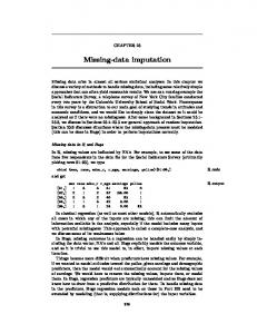
Constructing generative models to generate random images with certain texture structure is an important task in computer vision. A line of texture synthesis research proceeds by first extracting a set of features that characterizes the target texture and then generate images that match the features. The seminal work of Zhu et al. (1998) proposes constructing texture models under the ME framework, where features (or filters) of the given texture image are adaptively added in the model and a Gibbs distribution whose expected feature matches the target texture is learnt. One major difficulty with the method is that both model learning and image generation involve sampling from a complicated Gibbs distribution. More recent works exploit more complicated features (Portilla & Simoncelli, 2000; Gatys et al., 2015; Ulyanov et al., 2016). Ulyanov et al. (2016) proposes the texture net, which uses a texture loss function by using the Gram matrices of the outputs of some convolutional layers of a pre-trained deep neural network for object recognition. While the use of these complicated features does provide high-quality synthetic texture images, that work focuses exclusively on generating images that match these feature (moments). Importantly, this network focuses only on generating feature-matching images without using the ME framework to promote the diversity of the samples. Doing so can be deeply problematic: in Figure 1 (middle panel), we showed the lack of diversity resulting from only moment matching in that Dirichlet setting, and further we note that the extreme pathology would result in a point mass on the training image – a global optimum for this objective, but obviously a terrible generative model for synthesizing textures. Ideally, the MEFN will match the moments and promote sample diversity. We applied MEFN to texture synthesis with an RGB representation of the 224 × 224 pixel images , z ∈ Z = [0, 1]d , where d = 224 × 224 × 3. We follow Ulyanov et al. (2016) (we adapted https://github.com/ProofByConstruction/texture-networks) to create a texture loss measure T (z) : [0, 1]d → R, and aim to sample a diverse set of images with small moment violation. For the transformation family F we use the real NVP network structure proposed in Dinh et al. (2016) (we adapted https://github.com/taesung89/real-nvp). We use 3 residual blocks with 32 feature maps for each coupling layer and downscale 3 times. For fair comparison, we use the same real NVP structure for both1 , implemented in TensorFlow (Abadi et al., 2016). As is shown in top row of figure 3, both methods generate visually pleasing images capturing the texture structure well. The bottom row of Figure 3 shows that texture cost (left panel) is similar for both methods, while MEFN generate figures with much larger entropy than the texture network formulation (middle panel), which is desirable (as previously discussed). The bottom right panel of figure 3 compares the marginal distribution of the RGB values sampled from the networks: we found that MEFN generates a more variable distribution of RGB values than the texture net. We compute in Table 1 the average pairwise Euclidean distance between randomly sampled images (dL2 = meani6=j kzi − zj k22 ), and MEFN gives higher dL2 , quantifying diversity across images. We also consider an ANOVA-style analysis to measure the diversity of the images, where we think of the RGB values for the same pixel across multiple images as a group, and compute the within and between group variance. Specifically, denoting zik as the pixel value forP a specific pixel k = 1, ..., d for an image i = 1, ...., n. We partition the total sum of square SST = i,k (zik − z¯)2 as the within 1 Ulyanov et al. (2016) use a quite different generative network structure, which is not invertible and is therefore infeasible for entropy evaluation, so we replace their generative network by the real NVP structure

7

Under review as a conference paper at ICLR 2017

Input

Texture net (Ulyanov et al., 2016)

Texture cost Texture nets MEFN

10 8 10 7 10 6 0

5000 10000150002000025000 Iteration

RGB histogram 2.5 2.0 Density

10 9

Entropy 10 6 Negative Entropy

Texture cost

10 10

MEFN (ours)

10 5

1.5 1.0 0.5

10 4 0

0.0 0.0

5000 10000150002000025000 Iteration

0.2

0.4 0.6 RGB value

0.8

Figure 3: Analysis of texture synthesis experiment. See text for description. P P k group error SSW = ¯k )2 and between group error SSB = z k − z¯)2 , where i,k (zi − z i,k n(¯ z¯ and z¯k are the mean pixel values across all data and for a specific pixel k. Ideally we want the samples to exhibit large variability across images (large SSW, within a group/pixe) and no structure in the mean image (small SSB, across groups/pixels). Indeed, the MEFN has a larger SSW, implying higher variability around the mean image, a smaller SSB, implying the stationarity of the generated samples, and a larger SST, implying larger total variability also. The MEFN produces images that are conclusively more variable without sacrificing the quality of the texture, implicating the broad utility of ME. Table 1: Quantitative measure of image diversity using 20 randomly sampled images Method Texture net MEFN

5

dL2 11534 17014

SST 128680 175604

SSW 109577 161639

SSB 19103 13964

C ONCLUSION

In this paper we propose a general framework for fitting ME models. This approach is novel and has three key features. First, by learning a transformation of a simple distribution rather than the distribution itself, we are able to avoid explicitly computing an intractable normalizing constant for the ME distribution. Second, by combining stochastic optimization with the augmented Lagrangian method, we can fit the model efficiently, allowing us to evaluate the ME density of any point simply and accurately. Third, critically, this construction allows us to trivially sample iid from a ME distribution, extending the utility and efficiency of the ME framework more generally. Thus, accuracy equivalent to the classic Gibbs approach already would in itself be a contribution (owing to these other features); we also show that as the distribution increases in dimension, our MEFN approach outperforms Gibbs. We illustrate the MEFN in both a simulated case with known ground truth and real data examples. ACKNOWLEDGMENTS We thank Evan Archer for normalizing flow code, and Xuexin Wei, Christian Andersson Naesseth and Scott Linderman for helpful discussion. This work was supported by a Sloan Fellowship (JPC).

8

1.0

Under review as a conference paper at ICLR 2017

R EFERENCES Martın Abadi, Ashish Agarwal, Paul Barham, Eugene Brevdo, Zhifeng Chen, Craig Citro, Greg S Corrado, Andy Davis, Jeffrey Dean, Matthieu Devin, et al. Tensorflow: Large-scale machine learning on heterogeneous distributed systems. arXiv preprint arXiv:1603.04467, 2016. Adam L Berger, Vincent J Della Pietra, and Stephen A Della Pietra. A maximum entropy approach to natural language processing. Computational linguistics, 22(1):39–71, 1996. Thomas B Berrett, Richard J Samworth, and Ming Yuan. Efficient multivariate entropy estimation via k-nearest neighbour distances. arXiv preprint arXiv:1606.00304, 2016. Dimitri P Bertsekas. Constrained optimization and Lagrange multiplier methods. Academic press, 2014. Oleg Bondarenko. Estimation of risk-neutral densities using positive convolution approximation. Journal of Econometrics, 116(1):85–112, 2003. Jonathan Borwein, Rustum Choksi, and Pierre Mar´echal. Probability distributions of assets inferred from option prices via the principle of maximum entropy. SIAM Journal on Optimization, 14(2): 464–478, 2003. Peter W Buchen and Michael Kelly. The maximum entropy distribution of an asset inferred from option prices. Journal of Financial and Quantitative Analysis, 31(01):143–159, 1996. Michael Collins, Robert E Schapire, and Yoram Singer. Logistic regression, adaboost and bregman distances. Machine Learning, 48(1-3):253–285, 2002. John N Darroch and Douglas Ratcliff. Generalized iterative scaling for log-linear models. The annals of mathematical statistics, pp. 1470–1480, 1972. Stephen Della Pietra, Vincent Della Pietra, and John Lafferty. Inducing features of random fields. IEEE transactions on pattern analysis and machine intelligence, 19(4):380–393, 1997. Laurent Dinh, Jascha Sohl-Dickstein, and Samy Bengio. Density estimation using real nvp. arXiv preprint arXiv:1605.08803, 2016. Miroslav Dudik, Steven J Phillips, and Robert E Schapire. Performance guarantees for regularized maximum entropy density estimation. In International Conference on Computational Learning Theory, pp. 472–486. Springer, 2004. Stephen Figlewski. Estimating the implied risk neutral density. 2008. Leon Gatys, Alexander S Ecker, and Matthias Bethge. Texture synthesis using convolutional neural networks. In Advances in Neural Information Processing Systems, pp. 262–270, 2015. Arthur Gretton, Karsten M Borgwardt, Malte J Rasch, Bernhard Sch¨olkopf, and Alexander Smola. A kernel two-sample test. Journal of Machine Learning Research, 13(Mar):723–773, 2012. Edwin T Jaynes. Information theory and statistical mechanics. Physical review, 106(4):620, 1957. Jiantao Jiao, Kartik Venkat, Yanjun Han, and Tsachy Weissman. Minimax estimation of functionals of discrete distributions. IEEE Transactions on Information Theory, 61(5):2835–2885, 2015. Diederik Kingma and Jimmy Ba. Adam: A method for stochastic optimization. arXiv preprint arXiv:1412.6980, 2014. Diederik P Kingma and Max Welling. arXiv:1312.6114, 2013.

Auto-encoding variational bayes.

arXiv preprint

Robert Malouf. A comparison of algorithms for maximum entropy parameter estimation. In proceedings of the 6th conference on Natural language learning-Volume 20, pp. 1–7. Association for Computational Linguistics, 2002. Shakir Mohamed and Balaji Lakshminarayanan. Learning in implicit generative models. arXiv preprint arXiv:1610.03483, 2016. 9

Under review as a conference paper at ICLR 2017

Steven J Phillips, Robert P Anderson, and Robert E Schapire. Maximum entropy modeling of species geographic distributions. Ecological modelling, 190(3):231–259, 2006. Javier Portilla and Eero P Simoncelli. A parametric texture model based on joint statistics of complex wavelet coefficients. International journal of computer vision, 40(1):49–70, 2000. Danilo Jimenez Rezende and Shakir Mohamed. Variational inference with normalizing flows. arXiv preprint arXiv:1505.05770, 2015. Ruslan Salakhutdinov, Sam Roweis, and Zoubin Ghahramani. On the convergence of bound optimization algorithms. In Proceedings of the Nineteenth conference on Uncertainty in Artificial Intelligence, pp. 509–516. Morgan Kaufmann Publishers Inc., 2002. Dmitry Ulyanov, Vadim Lebedev, Andrea Vedaldi, and Victor Lempitsky. Texture networks: Feedforward synthesis of textures and stylized images. arXiv preprint arXiv:1603.03417, 2016. Paul Valiant and Gregory Valiant. Estimating the unseen: improved estimators for entropy and other properties. In Advances in Neural Information Processing Systems, pp. 2157–2165, 2013. Matthew D Zeiler. Adadelta: an adaptive learning rate method. arXiv preprint arXiv:1212.5701, 2012. Song Chun Zhu, Yingnian Wu, and David Mumford. Filters, random fields and maximum entropy (frame): Towards a unified theory for texture modeling. International Journal of Computer Vision, 27(2):107–126, 1998.

10

Under review as a conference paper at ICLR 2017

A

R ISK - NEUTRAL ASSET PRICE

We extract the risk-neutral asset price probability distribution based on option prices, an active and interesting area for ME models. We give a brief introduction of the problem and refer interested readers to see Buchen & Kelly (1996) for a more detailed explanation. Denoting St as the price of an asset at time t, the buyer of a European call option for the stock that expires at time te with strike price K will receive a payoff of cK = (Ste − K)+ = max(Ste − K, 0) at time te . Under the efficient market assumption, the risk-neutral probability distribution for the stock price at time te satisfies: cK = D(te )Eq [(Ste − K)+ ], (11) where D(te ) is the risk-free discount factor and q is the risk-neutral measure. We also have that, under the risk-neutral measure, the current stock price S0 is the discounted expected value of Ste : S0 = D(te )Eq (Ste ).

(12)

When given m options that expire at time te with strikes K1 , ..., Km and prices cK1 , ..., cKm , we get m expectation constraints on q(Ste ) from Equation 11, together with Equation 12, we have m + 1 expectation constraints in total. With that partial knowledge we can approximate q(Ste ), which is helpful for understanding the market expected volatility and identify mispricing in option markets, etc. Inferring the risk-neutral density of asset price from a finite number of option prices is an important question in finance and has been studied extensively (Buchen & Kelly, 1996; Borwein et al., 2003; Bondarenko, 2003; Figlewski, 2008). One popular method proposed by Buchen & Kelly (1996) estimates the probability density as the maximum entropy distribution satisfying the expectation constraints and a positivity support constraint by fitting a Gibbs distribution, which results in a piece-wise linear log density: ) ( m X ηi (z − Ki )+ 1 (z ≥ 0) (13) p(z) ∝ exp η0 z + i=1

and optimize the distribution with numerical methods. Here we compare the performance of the MEFN algorithm with the method proposed in Buchen & Kelly (1996). To enforce the positivity constraint we choose g(z) = eaz+b , where a and b are additional parameters. We collect the closing price of European call options on Nov. 1 2016 for the stock AAPL (Apple inc.) that expires on te = Jun. 16 2017. We use m = 4 of the options with highest trading volume as training data and the rest as testing data. On the left panel of figure 4, we show the fitted risk-neutral density of Ste by MEFN (red line) with that of the fitted Gibbs distribution result (blue line). We find that while the distributions share similar location and variability, the distribution inferred by MEFN is smoother and arguably more plausible. In the middle panel we show a Q-Q plot of the quantiles of the MEFN and Gibbs distributions. We can see that the quantile pairs match the identity closely, which should happen if both methods recovered the exact same distribution. This highlights the effectiveness of MEFN. There does exist a small mismatch in the tails: the distribution inferred by MEFN has slightly heavier tails. This mismatch is difficult to interpret: given that both the Gibbs and MEFN distributions are fit with option price data (and given that one can observe at most one value from the distribution, namely the stock price at expiration), it is fundamentally unclear which distribution is superior, in the sense of better capturing the true ME distribution’s tails. On the right panel we show the fitted option price for the two fitted distributions (for each strike price, we can recover the fitted option price by Equation 11). We noted that the fitted option price and strike price lines for both methods are very similar (they are mostly indiscernible on the right panel of figure 4). We also compare the fitted performance on the test data by computing the root mean square error for the fitted and test data. We observe that the predictive performances for both methods are comparable. We note that for this specific application, there are practical concerns such as the microstructure noise in the data and inefficiency in the market, etc. Applying a pre-processing procedure and incorporating prior assumptions can be helpful for getting a more full-fledged method (see e.g. Figlewski (2008)). Here we mainly focus on illustrating the ability of the MEFN method to approximate the ME distribution for non-typical distributions. Future work for this application includes fitting a riskneutral distribution for multi-dimensional assets by incorporating dependence structure on assets. 11

300

Gibbs MEFN

identity

250

Option price (dollars)

0.035 0.030 0.025 0.020 0.015 0.010 0.005 0.000

MEFN Quantiles

Density

Under review as a conference paper at ICLR 2017

200 150 100 50

0

50

100 150 Price (dollars)

200

0

0

50

100 150 Gibbs Quantiles

200

250

120 100 80 60 40 20 0 20

Gibbs, RMSE=2.43 MEFN, RMSE=2.39 Training data Testing data

0

50 100 150 Strike price (dollars)

Figure 4: Constructing risk-neutral measure from observed option price. Left panel: fitted riskneutral measure by Gibbs and MEFN method. Middle panel: Q-Q plot for the quantiles from the distributions on the left panel. Right panel: observed and fitted option price for different strikes.

12