RMZ - Materials and Geoenvironment, Vol. 53, No. 3, pp. 323-338, 2006
323
Maximum Entropy Theory by Using the Meandering Morphological Investigation Levent Yilmaz Technical University of Istanbul, Hydraulic Division, Civil Engineering Department, Maslak, 80626, Istanbul, Turkey.; E-mail:
[email protected] Received: November 02, 2006
Accepted: November 14, 2006
Abstract: Based on the principle of maximum entropy the primary morphologic equation is derived, and then the equations for hydraulic geometry of longitudinal profile and crosssection are established. For V-shaped cross-sections the relevant morphologic equations which are derived are compared with the existing empirical and semi-empirical formulae. They show good agreement with the prototypes. Key words: Principle of maximum entropy, hydraulic geometry, morphologic equation
Introduction Einstein (1950) once pointed out that entropy theory is the first theory for overall science. The principle of maximum entropy has been extensively applied in many domains of natural science. In view of this fact, to apply the principle of maximum entropy is adopted to deal with characteristics of alluvial channels capable of carrying given water and sediment load in meandering boundary layers without causing excessive aggradation and degradation. Width adjustment may take place over a wide range of scales in time and space at meandering channels. In the past engineering analyses of channel width have tended to concentrate on prediction of the equilibrium width for stable channels. Most commonly the regime; extremal hypothesis, and rational (mechanistic) approaches are used. By meandering channels, more Scientific paper
recently, attention has switched to channels that are adjusting their morphology either due to natural instability or in response to changes in meandering watershed land use, river regulation, or channel engineering. Characterizing and explaining the time-dependent behavior of width in such channels requires and understanding of the fluvial hydraulics of unstable channels, especially in the near-bank regions. Useful engineering tools are presented, and gaps requiring further field and laboratory research are identified. Finally, this research will consider the mechanics of bank retreat due to flow erosion and deposition at meandering bends, mass failure under gravity, and bank advance due to sedimentation and berm building. It will be demonstrated that, while rapid progress is being made, most existing analyses of bank mechanics are still at the stage of being research tools that are not yet suitable for design applications.
324
Most mathematical models, however, neglect time- dependent channel width adjustments and do not simulate processes of bank erosion or deposition at meandering channels. Although changes in channel depth caused by aggradation or degradation of the river bed can be simulated, changes in width cannot. Meandering channel morphology usually changes with time, and adjustment of both width and depth, in addition to changes in planform, roughness, and other attributes are the rule rather than the exception (Leopold et al., 1964; Simon and Thorne, 1996). As a result, the ability to model and predict changes in river morphology and their engineering impacts is limited. The meandering river width adjustments can seriously impact floodplain dwellers, riparian ecosystems, bridge crossings, bank protection works, and other riverside structures, through bank erosion, bank accretion, or bankline abandonment by the active river channel, which are very important for sustainable development of European Mediterranean countries. Considerable research effort has recently been directed towards improving this situation. The objectives of the river width adjustment research were as follows: • Review the current understanding of the fluvial processes and bank mechanics involved in river width adjustment • Evaluate methods (including regime analysis, extremal hypotheses and rational, mechanistic approaches) for predicting equilibrium river width • Assess the present capability to quantify and model width adjustment • Identify current needs to advance both state-of-the-art research and the solution of real world problems faced by practicing engineers
Yilmaz, L.
To achieve these objectives, river width adjustments may occur due to a wide range of morphological changes and channel responses. Widening can occur by erosion of one or both banks without substantial incision (Everitt, 1968; Burkham, 1972; Hereford, 1984; Pizzuto, 1992). Widening in sinuous channels may occur when outer bank retreat, due to toe scouring, exceeds the rate of advance of the opposite bank, due to alternate or point bar growth (Nanson and Hickin, 1983: Pizzuto, 1994) while, in braided rivers, bank erosion by flows deflected around growing braid bars is a primary cause of widening (Leopold and Wolman, 1957; Best and Bristow, 1993; Thorne et al., 1993). In degrading streams, widening often follows incision of the channel when the increased height and steepness of the banks causes them to become unstable. Bank failures can cause very rapid widening under these circumstances (Thorne et al., 1981; Little et al., 1982; Harvey and Watson, 1986; Simon, 1989). Widening in coarse-grained, aggrading channels can occur when flow acceleration due to a decreasing cross-sectional area, coupled with current deflection around growing bars, generates bank erosion (Simon and Thorne, 1996). Morphological adjustments involving channel narrowing are equally diverse. Rivers may narrow through the formation of in-channel berms, or benches at the margins. Berm/bench growth often occurs when bed levels stage following a period of degradation and can eventually create a new, lowelevation floodplain and establish a narrower, quasi-equilibrium channel (Woodyer, 1968; Harvey and Watson, 1986; Simon, 1989; Pizzuto, 1994). Narrowing in sinuous channels occurs when the rate of alternate or point bar RMZ-M&G 2006, 53
Maximum Entropy Theory by Using the Meandering Morphological Investigation
growth exceeds the rate of retreat of the cut bank opposite (Nanson and Hickin, 1983; P izzuto , 1994). Croachment of riparian vegetation into the channel is often satisfied as contributing to the growth, stability, and initiation of berm or bench features (Hadley, 1961; Schumm and Lichty, 1963; Harvey and Watson, 1986; Simon, 1989). In braided channels, narrowing may result when a marginal anabranch in the braided system is abandoned (Schumm and Lichty, 1963). Sediment is deposited in the abandoned channel until it merges into the floodplain. Also, braid bars or islands may become attached to the floodplain, especially following a reduction in the formative discharge. Island tops are already at about floodplain elevation and attached bars are built up to floodplain elevation by sediment deposition on the surface of the bar, often in association with establishment of vegetation. Attached islands and bars may, in time, become part of the floodplain bordering a much narrower, sometimes single-threaded channel (Williams, 1978; Nadler and Schumm, 1981). If the flow regime and sediment supply are quasi-steady over periods of decades, the morphology of the river adjusts to create a metastable, equilibrium form (Schumm and Lichty, 1965). Such rivers are described as being graded or in regime (Mackin, 1948; Leopold and Maddock, 1953; Wolman, 1955; Leopold et al. 1964; Ackers and Charlton, 1970a). Although the width of an equilibrium stream may change due to the impact of a large flood or some other extreme event, the stable width is eventually recovered following such perturbations (Costa, 1974; Gupta and Fox, 1974; Wolman and Gerson, 1978). Unfortunately, predicting the time-averaged morphology of equilibrium RMZ-M&G 2006, 53
325
channels remains, despite years of effort, a difficult problem (Ackers, 1992; Ferguson, 1986; Bettess and White, 1987). Many rivers, however, cannot be considered to have equilibrium channels even as an engineering approximation. These rivers display significant morphological changes. Under the assumption that the only information available on a drainage basin is its mean elevation, the connection between entropy and potential energy is explored to analyze drainage basins morphological characteristics. Nearly, 30 years ago, Leopold and Langbein (1962) applied for the first time the concepts of physical entropy to study the behavior of streams. Their application was based on the analogy between heat energy and temperature in a thermodynamic system and potential energy and elevation, respectively, in a stream system. Two thermodynamic principles were applied. The first principle is that the most probable state of a system is the one of maximum entropy. The second is the principle of minimum entropy production rate. Using these principles, Yang (1971) derived for a stream system the law of average stream fall, and the law of the least rate of energy expenditure. Yang (1971) and others have since applied the latter law to a range of problems in hydraulics. The connection between entropy and potential energy, which these workers so successfully exploited to investigate river engineering, sediment transport, and other problems, was not exploited in hydrology. In this work we pursue this connection to derive relations between entropy and mean elevation for a drainage basin network and to derive relations for the river profiles.
326
Yilmaz, L.
Much of the work employing the entropy concepts in hydrology has been with the application of informational entropy. The beginnings of such a work can be traced to Lienhard (1964), who used a statistical mechanical approach to derive a dimensionless unit hydrograph of a drainage basin. It may be visualized that the study of the landscape is the study of constraints imposed by geologic structure, lithology, and history. The way in which some constraints affect the river profile can be evaluated if one considers the profile to approximate its maximum probable condition under a given set of constraints. The most important observations are summarized as below: a) The absence of all constraints leads to no solution. b) The longitudinal profile of a stream system subject only to the constraint of base level is exponential with respect to elevations above base level. c) The profile of a stream subject only to the constraint of length is exponential with respect to stream length which is a logarithmic function with respect to elevation. d) Introduction of the constraint of a partial base level above that of the sea adds a measure of convexity in the profile.
Principle of maximum discrete entropy
For a discrete variable X, Shannon (1948) defines quantitatively the entropy in terms of probability as:
(1)
where P(Xi) is the probability of a system being in state Xi which is a member of {Xi, i = 1, 2, …}, and It has been proved that H(X) defined by Equation 1 is the only function to satisfy the following three conditions: a) H(X) is the continuous function of P(Xi). b) If and only if all P(Xi) are equal, H (X) attains its maximum value. This conclusion is known as the principle of maximum discrete entropy. c) If the states X and Y are mutually independent, then H(XY) = H(X)+H(Y). Jaynes (1957) have proved that an equilibrium system under steady constraints tends to maximize its entropy. Based on this statement, the entropy of a river system, having reached its dynamic equilibrium, should approach its maximum value, also the principle of maximum entropy should be valid too for the case of regime rivers. Stream Power Although many formulas for sediment transport have been devised, most can be expressed in terms of stream power as suggested by Bagnold (1960). Power is an important factor in the formulation of the hydraulic geometry of river channels. As explained by Bagnold, the stream power at flows sufficiently great to be effective in shaping the river channel is directly related to the transport of sediment, whose movement is responsible for the channel morphology. Laursen (1958) gives several typical equations for the transport of sediment, based on flume experiments and the average relation shows sediment transport RMZ-M&G 2006, 53
Maximum Entropy Theory by Using the Meandering Morphological Investigation
in excess of the point of incipient motion to vary about as (vDS)1.5 where vDS is the stream power per unit area. In terms of sediment per unit discharge, that is the concentration, C, the several equations average out as C ∝ n (vD)0.5 S1.5, a result that is consistent with the conclusion reached by Bagnold (1960). There is in addition to be considered the effect of sediment size. Examination of several equations indicates that sediment transport varies inversely as about the 0.8 power of the particle size. There have been several attempts to relate particle size to the friction factor n and by using the Strickler relation that the value of n varies as the 1/6 power of the particle size. It is realized full well that both the sediment transport and the friction factor are influenced by many other factors such as bed form and the cohesiveness, sorting, and texture of the material. These are the kinds of influences, themselves effects of the river, that prevent a straightforward solution of river morphology. In order to limit the number of variables only the effect of particle size on transport will be considered, as this factor varies systematically along a river from headwater to mouth. Thus, sediment transport concentration is given as C ∝ (vD)0.5 S1.5 / n4. The sediment transport per unit discharge in the river system will be recognized as a hydrologic factor that is independent of the hydraulic geometry of a river in dynamic equilibrium. Consequently sediment concentration may be considered constant. Thus, there are three equations: continuity, hydraulic friction, and sediment transport. There are five unknowns. The two remaining equations will be derived from a consideration of the most probable distribution of energy and total energy in the river system. RMZ-M&G 2006, 53
327
The probability of a given distribution of energy is the product of the exponential functions of the ratio of the given units to the total as (1a) The ratios of the units of energy E1, E2, etc., representing the energy in successive reaches along the river sufficiently long to be statistically independent, to the total energy E in the whole length, are E1/E ; E2/E; …… En/E. The product of the exponentials of these is the probability of the particular distribution of energy. As previously, the most probable condition is when this joint probability, p, is a maximum and this exists when E1 = E2 = E3 … = En. Thus energy tends to be equal in each unit length of channel (Leopold and Langbein, 1962). Equable distribution of energy corresponds to a tendency toward uniformity of the hydraulic properties along a river system. Considering the internal energy distribution, uniform distribution of internal energy per unit mass is reached as the velocity and depth tend toward uniformity in the river system. Since the energy is largely expended at the bed equable distribution of energy also requires that stream power per unit of bed area tend toward uniformity. An opposite condition is indicated by Prigogine’s (1955) rule of minimization of entropy production which leads to the tendency that the total rate of work, ∑QS∆Q in the system as a whole be a minimum. Because S ∝ Qz, then ∑Q1+z ∆Q→a minimum. For a given drainage basin this condition is met as z takes on increasingly large negative values. However, there is a physical limit on the value of z,
328
Yilmaz, L.
because for any drainage basin the average slope ∑S∆Q/∑∆Q must remain finite. This condition is met only for values of z greater than –1, and therefore z must approach –1 or 1 + z approaches zero. The condition of minimum total work tends to make the profile concave; whereas the condition of uniform distribution of internal energy tends to straighten the profile. Hence, we seek the most probable state. The most probable combination is the one in which the product of the probabilities of deviations from expected values is a maximum. It is unnecessary to evaluate the probability function, provided one can assume normality, as we can then state directly that the product of the separate probabilities is a maximum when their variances are equal.
the solution is not sensitive to the values of the several standard deviations, so the solution converges rapidly. Therefore,
(3) for which there are two possible solutions:
(4) or
(5) To summarize, we have introduced three statements on the energy distribution:
(2) where F1, F2, F3 represent the several functions. The standard deviations σm, σf, σz, and σy represent the variability of the several factors as may occur along a river system. Since these values are not known initially, the problem must be solved by iteration (Leopold and Langbein, 1962). Fortunately,
(6), (7),(8) The absolute values of the standard deviations need not be known, as we can infer their relative values. For example, letting F1 = (1/2)z – y , the standard deviation of F1 is (9)
RMZ-M&G 2006, 53
Maximum Entropy Theory by Using the Meandering Morphological Investigation
329
and F2=m+f+z
(10)
L eopold and M addock (1953) describe and evaluate from field data the hydraulic geometry of river channels by a set of relations as follows: v∝Qm
(11)
D∝Qf
(12)
w∝Qb
(13)
S∝Qz
(14)
n∝Qy
(15)
where v is the mean velocity, D is the mean depth, w is the surface width, and S is the energy slope, and n is the friction factor at a cross section along a river channel where the mean discharge is Q. It is desired to evaluate the exponents in a downstream direction as discharge of uniform frequency increases. Some of the principles that have been described can provide estimates of the magnitude of the exponents of the above relationships. The exponents m, f, b, z, and y describe the variability in velocity, depth, width, slope, and friction along a river channel, but do not uniquely determine the magnitudes of these properties. The first condition is that specified by the equation of continuity Q=vDw, which requires that m + f + b = 1.0
RMZ-M&G 2006, 53
(16)
The solution of their values is not available for the first trial solution so all values are considered equal. Thus:
(17)
(18)
(19)
The results of the first solution are then used to derive first estimates of the standard deviations, and a second computation carried forward. A third calculation is made to confirm the results of the second trial solution. These three equalities lead to two independent equations y = - ½ (m + f)
(20)
z = - 0.53 + 0.93 y
(21)
which, together with the three hydraulic conditions m + f + b = 1.0
(22)
m = (2/3)m + (1/2)z – y
(23)
(1/2)m = (1/2)f + 1.5 z – 4y = 0
(24)
330
Yilmaz, L.
lead to a solution for m, f, b, z, and y. The final values, derived without reference to field data, are compared below with others obtained previously from analysis of field data on actual rivers. Table 1. Values of exponents of the hydraulic geometry in downstream direction ( Leopold and Maddock, 1953)
Theoretical values Velocity, m = 0.09 Depth, f = 0.36 Width, b = 0.55 Slope, z = - 0.74 Friction, y = - 0.22
Average values from data on rivers m = 0.10 f = 0.40 b = 0.50 z = - 0.49
Velocity is such a large factor in energy expenditure, the value of m, the exponent of velocity, is close to zero, making this characteristic the most conservative. The value of z which is the measure of the variability in slope is least satisfactorily defined from field data, as it is affected by variation in the friction factor. Thus, the value of z as reported above is – 0.53 + 0.93 y. Hence the value of z is – 0.53 where grain size is constant. The value of z was found by Leopold (1953) to be – 0.49 for midwestern rivers. Henderson (1961) shows that for a stable channel of uniform grain size the slope varies as the – 0.49 power of the discharge (Table 1). However, when a large variety of river data were averaged, including data on ephemeral channels, Leopold and Miller (1956) obtained a value of z averaging near z = - 0.95. Values of z in excess of 0.50 may be attributed to the common tendency for the friction factor to decrease downstream by increasing discharge as particle size decreases. In canals, for example, where y
is positive, the value of z is less than 0.50 (Leopold and Langbein, 1962). The study of hydraulic geometry develops a method of solution through introduction of probability statements. The results which are obtained by this theoretical derivation of exponents in the hydraulic geometry agree quite well with field data , but we are far from satisfied physical relationships. For example, there is uncertainty whether the transport equations represent physical relationships or are in fact formulas for sediment transport under regime conditions. Several alternative assumptions were tried and the resulting exponents also agreed quite well with field data. Drainage Network In the longitudinal profile, the probability that a random walk will fall in certain positions within the given constraints can be ascertained. There is also a mean or most probable position for a random walk within those constraints. This statement suggests the possibility that a particular set of constraints might be specified that would describe the physical situation in which drainage channels would develop and meet. If the precipitation falls on a uniformly sloping plain which develops an incipient set of rills near the watershed, the rills deepen with time and crossgrading begins owing to overflow of the shallow incipient rills. The direction that the crossgrading takes place is a matter of chance until the rills deepen sufficiently to become master rills. The randomness in the first stages of crossgrading might be approximated in the conceptual model which is amenable to mathematical description. Considering a series of initial points on a line and equidistant from one another at spacing a and assuming random walks originating at each of these points. RMZ-M&G 2006, 53
Maximum Entropy Theory by Using the Meandering Morphological Investigation
Experimental setup A movable laboratory channel with varying slope was installed for investigating the meander evolution, measuring the erosion rate, and studying the sediment-water interaction in the meandering channel. On the bottom of the channel that is filled with the cohesionless sand, a straight initial channel that was to follow a meandering path during flow was carved. Discharge, slope of the main channel, and sediment transport rate were observed during the meandering plan-formation. The main channel was 10 m long, 1.60 m wide, and 0.42 m deep. The original channel was filled through a feedback system with a uniform sand of 1.35 mm of median diameter up to a depth of 0.30 m. A movable carriage was mounted on the 8.80 m long side rails for measuring the channel and sediment-flow characteristics. Water coming from the head tank was passed through a water tranquilizer, which was 1.60 m wide, 0.26 m long, and 0.65 m deep. The sediment supplier for the feedback system was laid at the entrance, but after the tranquilizer. The downstream reservoir for outflow with the end gate (0.15 m wide and 0.15 m high) was 1.10 m long, 1.60 m wide, and 0.65 m deep. The sand collector (0.42 m x 1.60m x 0.65m) was placed at the end of the channel. Into the uniform sand (of 1.35 mm of median diameter) of the 8.80 m long flume channel, a trapezoidal cross-section was carved, with a bottom width = 0.10 m, water width = 0.20 m, and flow depth = 0.10 m. The movable carriage on the side rails was used for setting the profile indicator instrument and the velocity measurement instrument for obtaining the geomorphological and RMZ-M&G 2006, 53
331
physical characteristics of the meandering channel. In experimentation, it was possible to change the slope, discharge, and other hydraulic parameters. For exact measurements of the sediment transport rate, a Sartorius weight measuring instrument was placed at the end of the channel. The sediment washed down from the flume was collected with a sieve in the downstream reservoir. It was dried and weighed with the Sartorius weight measuring instrument for computing the total sediment transport rate.
Experimental observations The experimental model in the present study consists of a very simple straight channel, which, after some time, converts to meander planforms on the sandy bottom of the main channel. Thus, the experimental setup seems to mimic a natural meandering river, for it reflects the development of a meandering channel on the cohesionless bottom boundary layer, exhibiting every phase from the beginning to the end of the erosion event at the bank and the bottom boundary layer. However, one of the limitations of the experimental setup was its inability to observe braiding planforms. It was seen that there was no sediment transport after meandering and the stability of the flume was observed with the development of the meandering planform. Since flow exerts shear stresses that can remove particles from the banks and the near-bank flow pattern is determined by discharge, the influence of only discharge was taken into account in the experimental investigation. Observations for the transported bed material weight in time were taken for Q = 0.1536 l/s and S = 0.08 %, and these
332
are presented in this study. However, the main channel slope could be varied between 0.04–0.5 % and the main channel discharge between 0.07–0.73 l/s. Measurements could not be made for experimental limitations beyond this range. For example, the flow in the flume of sandy bottom changed from subcritical to supercritical regime as the slope increased beyond the given range. Furthermore, more versatile equations for bed load transport and for meandering bend planform are required to deal with supercritical flows. In the case of high flows, the zone of maximum bedload transport shifted outward through the bend. Over 80% of the bed load in transport traveled to the right (closer to the inside bank) of the centerline in the upstream part of the bend. In the downstream portion of the bend, over 50% traveled to the left (closer to the outside bank) of the centerline. The temporal variation of the total dry mass of the collected sediment amount is depicted. Dividing the total dry weight of the collected sediment amount by the sediment-collection time yields the average sediment transport rate in mass per unit time. Sand transport varied from 21–200 gm per hour during 320 hours of the experiment. The sandwater mixture introduced into the initial straight channel caused it to transform to the meandering form after 320 hours, the time after which an equilibrium condition was reached. Here, the equilibrium condition infers no sediment transport condition. In the developing meandering channel, bed profiles and velocities were measured by the profile indicator and velocity-measurement instruments.
Yilmaz, L.
It was observed that the slope of the channel increased as it developed from the straight form through a shoaled condition to the meandering pattern, and that this channel pattern was associated with significantly higher sediment transport rates than the straight form. To prevent the channel from overflowing due to the increasing bed slope at the head of the system, a constant small freeboard was maintained during experimentation.
Analysis of Experimental Measurements Modeling of Sediment Transport Rates Utilizing the laboratory observations, two equations were developed: one for bed load transport and the other for meander planform. This involves (1) an investigation of sediment transport in the laboratory flume, considering the prototype, and (2) development of an experimental meander bend equation. Sediment–transport processes lead to meandering planforms at the flume-bank erosion and consequently, to flume widening. Using the sediment transport measurements, the correlation between the sediment transport change and meandering planform was analyzed. To that end, an attempt was made to begin the experimental procedure with first ‘measuring the sediment transport’ and then ‘measuring the meander bend formation’. For the above Q- and S-values, the measurements of the sediment transport rates for the whole period of 320 hrs are depicted. It is apparent from this figure that there exists a specific value of the sediment rate at time equal to zero. It is for the reason that the sediment load was supplied through the feedRMZ-M&G 2006, 53
Maximum Entropy Theory by Using the Meandering Morphological Investigation
back system just before the time of the start of experimentation. Soon afterwards, the rate increases sharply and then decreases in a fluctuating manner, but generally decays with time. The sudden kinks here and there in the graph are the result of sudden erosion of the bed and banks of the channel and its washing away to the end of the channel, where it is finally collected for measurements. The sudden washing away of the sediment particles is also attributed to the generation of secondary currents that augment the flow velocity because of the variation in the effective discharge due to the supplying of sediment load through feed-back system. After the occurrence of such a phenomenon, a reverse trend of decreasing sediment rate is visible. It occurs because of the negative role of secondary velocities, leading to the reduction of the effective downstream flow velocity. Ignoring these effects, the overall result is that the sediment rate decays almost exponentially with time and reaches almost a constant or equilibrium value after approximately 320 hrs. The decaying trend of the depicted sediment transport rates can be modeled by the following empirical relation: Qb = 1.5227 e-0.0091 t
(25)
with the correlation coefficient (R2) equal to 0.8993, indicating a reasonably good fit. In Equation 25, Qb is the total bed load in the experimental channel in kg/hr, t is the time in hour (after the beginning of meandering). It is noted that this equation is fitted to the observed data points excluding the points showing sudden kink at 115 and 225 hrs. It exhibits an intercept of 1.5227 kg/hr at time equal to 0 and sediment transport RMZ-M&G 2006, 53
333
rate approaches zero when time approaches infinity. Physically, the intercept indicates approximately the sediment transport rate supplied through the feed-back system at time t = 0. The disadvantage of the fitted model, however, is that the equilibrium condition reaches at t approaching infinity. On the other hand, this condition was practically observed between 250 and 320 hrs since the beginning of meandering. Thus, many more sets of observations will be required before finally recommending an equation of the kind of Horton (1945) infiltration model, which incorporates a static infiltration component analogous to the equilibrium condition of sediment transport rate achieved after a certain time. However, taking the value of this equilibrium condition equal to 0.165 kg/hr, Equation 25 is modified as: Qb = 0.1650+1.3577 e-0.0091 t
(26)
where the decay factor is equal to 0.0091 per hr. The development of such an equation is of significance for reason that the bed load molds the geometry of rivers. Since the shortduration (for example, 5 minutes or shorter) sand transport rates were not measured, Equations 25 and 26 may not be valid for the short-duration measurements and require a detailed investigation for the development of a comprehensive sand transport curve. Modeling of Channel Meander Planforms In channel meandering, flume erodibility is not the only limiting factor for cross-section widening. When a cross-section becomes very wide and shallow, its cross-sectional shape may become unstable and develop into a number of separate, narrower chan-
334
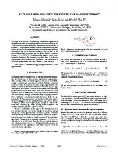
nels, thus transforming into a braided or an anabranching river. In the present experimentation, limited runs were taken only for achieving the meandering planforms and for braiding or anabranching river cross-sections, the experiment was not continued. The formation of the meandering channel at different times and in a specific channel reach of 250 cm is shown in Figure 1, in which x is the space coordinate in the flow direction, and y is the space coordinate in the normal direction. Since longitudinal planform changes were insignificant, only lateral planform changes were considered. It is apparent from Figure 1 that at time t increases the departure of the meandering channel (measured from the center of the initially straight channel) increases with time and at time t = 160 hrs, a fully developed meandering planform was observed. It is also apparent from this figure that the radius of curvature of the meander increases from 0 to 125 cm, where it is maximum, and then, continually decreases up to
Yilmaz, L.
250 cm. The apparent kinks in the meander planforms are the result of local changes in secondary currents of the flume. These planform changes can be modeled by a quadratic equation of the form: y = a x2 + b x + c
(27)
where y is the lateral departure of the meandering channel from the initially straight channel in the longitudinal direction x, and a through c are the parameters. The computed parameter values for time-varying planform changes are given in Table 1. It is seen from this table that the values of the coefficient of correlation range from 0.8405 to 0.9847 suggesting satisfactory fits to the planform changes. In an attempt to investigate the variation of the parameters of Equation 27 with the changing meandering planforms, these were correlated with time for making the planform model (Equation 27) fully predictive.
Table 2. Changes of parameter values of Equation 27 With Time.
Table 3. Fitting Values of Parameters M and C1 Of Equation 28
RMZ-M&G 2006, 53
Maximum Entropy Theory by Using the Meandering Morphological Investigation
Q = 0.08 l/s ; So= 0.08 %
Q = 0.20 l/s ; So=0.10%
Q = 0.40 l/s ; So = 0.20 %
Q = 0.50 l /s ; So= 0.35 % Figure 1. Fully developed meandering channel patterns for various of discharge (Q) and bed slopes (So) of the channel after 72 hours RMZ-M&G 2006, 53
335
336
Yilmaz, L.
In Table 3, the fitted relations for the parameters of Equation 28 with time exhibit the straight-line relationship: y1 = m x1 + c1
(28)
where y1 represents the parameter a, b, or c of Equation 27; x1 is the time (hr); and m and c1 represent the slope and intercept of the straight line, respectively. The computed values of the parameters of Equation 28 for the parameters a, b, and c of Equation 28 are summarized in Table 3. Apparently the computed values of R2 range from 0.9855-0.9971, exhibiting excellent fits. It is apparent from Table 2 that parameter ‘a’ grows linearly with time, and so does the parameter ‘c’. Parameter ‘b’, however, decreases with time. The consistent regular relationship of each parameter with time exhibits a sound predictability of the above meander planform model (Equation 27). It is interesting to note that all parameters exhibit a linear variation with time. However, the meandering phenomenon is a non-linear process, for the parameters change with time although linearly. The workability of the developed meandering model (Equation 27) and the parametric relations (Equation 28) is demonstrated by comparing the observed meander departures from the initially straight channel with the computed ones in Figure 1. In this figure, the line of perfect fit (LPF) indicates a perfect match between the observed and computed values. The values above and below the LPF indicate over- and underprediction by the model (Equation 27). It is seen that all the data points hover around the LPF, indicating a satisfactory prediction. The Nash and Sutcliffe’s (1970) efficiency is computed as equal to 97.2187, which shows an excellent model prediction.
Discussion and geomorphic results
The investigation shows that several geomorphic forms appear to be explained in a general way as conditions of most probable distribution of energy, the basic concept in the term “entropy”. The word entropy has been used in the development of systems other than thermodynamic ones, specifically, in geomorphological theory. Stream channels show in many ways the effects of previous climates, and of structural or stratigraphic relations that existed in the past. In some instances the present streams reflect the effects of sequences of beds which have been eradicated by erosion during the geologic past. However, these conditions that presently control or have controlled in the past the development of geomorphic features now observed need not be viewed as preventing the application of a concept of maximum probability. Rather, the importance of these controls strengthens the usefulness and generality of the entropy concept. In a sense, much of geomorphology has been the study of the same constraints that have been attempted to express in a mathematical model. The geomorphic results show that the present model should not be considered to deal with random walks. It is concerned with the distribution of energy in real landscape problems. The experimental model also give the proofs to this consideration.
RMZ-M&G 2006, 53
Maximum Entropy Theory by Using the Meandering Morphological Investigation
References Ackers, P., and Charlton, F. G., 1970a, Meander geometry arising from varying flows, Journal of Hydrology, Vol. 11, No.3, pp. 230-252. Bagnold, R. A., 1960, Sediment discharge and stream power – a preliminary announcement: U. S. Geol. Survey Circ. 421, 23 p. Best, J. L. and Bristow, C. S., 1993, A cellular model of braided rivers, Geological Society, London. p.113 Bettess, R., and White, W. R., 1987, Flood Mitigation Strategy for Medium-sized Streams, Canadian Water Resources, Vol. 11, pp. 132 – 141. Burkham, D. E., 1972, Channel changes of the Gila River in Safford Valley, Arizona 1846 – 1970, U.S. Geological Survey Professional Paper 655 –6. Da Costa, Newton C. A., 1974, On the theory of Inconsistent Formal Systems, NDJFL, Vol. 15, pp. 497 – 510. Einstein, H. A., 1950, The bed-load function for sediment transportation in open channel flows : Tech. Bull., U.S.D.A., Soil Conservation Service, No. 1026. Everitt, B. L., 1968, Use of the cottonwood in an investigation of the recent history of a floodplain, American Journal of Science, Vol. 266, pp. 417 – 439. Ferguson, R. I., 1986, Hydraulics and hydraulic geometry, Progress in Physical Geography, Vol. 10, pp. 1 – 31. Gupta, A, and Fox, H., 1974, Effects of High Magnitude Floods on Channel Form: A Case Study in the Maryland Piedmont, Water Resources Research, Vol: 10, pp. 499 – 509. Hadley, R. F., 1961, Progress in the application of landform analysis in studies of semiarid erosion, U. S. Geological Survey Circular, 437. Harvey, M. D., and Watson, C. C., 1986, Fluvial processes and morphologic thresholds in stream channel restoration, Water Resources Bulletin, Vol. 22, no:3, pp. 359 – 368. Henderson, F. M., 1961, Sediment Transport, Open Channel Flow, Chapter 10, MacMillan, New York. Hereford, R., 1984, Climate and ephemeral stream processes: Twentieth –Century geomorphology and alluvial stratigraphy of the Little Colorado River, Arizona: Geological Society of Amerika Bulletin, Vol. 95, pp. 654 – 668. RMZ-M&G 2006, 53
337
Horton, R. E., 1945, Erosional development of streams and their drainage basins; hydrophysical approach to quantitative morphology: Geol. Soc. America Bull., v. 56, p. 275-370. Jaynes, E. T., 1957, Information theory and Statistical mechanics, I, Physics Review, Vol. 106, pp. 620-630. Laursen, E. M., 1958, Sediment-transport mechanics in stable channel design: Am. Soc. Civil Engrs. Trans. V. 123, p. 195-206. Leopold, L. B., 1953, Downstream change of velocity in rivers: Am. Jour. Sci., v. 251, p. 606-624. Leopold, L. and T., Maddock, 1953, The hydraulic geometry of stream channels and some physiographic implications, U.S. Geological Survey Professional Papers, United States Government Printing Office, Washington. Leopold, L. B., and Maddock, T., Jr., 1953, The hydraulic geometry of stream channels and some physiographic implications: U. S. Geol. Survey Prof. Paper 252, 56 p. Leopold, L. B., and Miller, J. P., 1956, Ephemeral streams – Hydraulic factors and their relation to the drainage net: U. S. Geol. Survey Prof. Paper 282-A, p. 1 – 36. Leopold, L. B., and Wolman, M. G., 1957, River channel patterns; Braided, meandering and straight, USGS Professional Paper 282-B, pp. 45-62. Leopold, L. B. and LangbeinW. B., 1962, The concept of entropy in landscape evolution, Geological Survey Professional Paper, 500-A. Leopold, L. B., Wolman, M. G., and Miller, J. P., 1964, Fluvial processes in geomorphology, W. H. Freeman and Co., San Francisco, Calif., p. 522. Lienhard, J. H., 1964, A statistical mechanical prediction of the dimensionless unit hydrograph, Journal of Geophysical Research, Vol. 69, No: 24, pp. 5231. Little, A. D. and Curren, C. E., 1982, Archaeological Investigations in the Buttahatchee River Valley, Journal of Alabama Archaeological Society. Nadler, C. T. and S. A. Schumm, 1981, Metamorphosis of South Platte and Arkansas Rivers, Eastern Colorado, Physical Geography, Vol. 2, pp. 95 – 115. Nanson, G. C. and Hickin, E . J., 1983, Channel migration and incision on the Beatton River, ASCE, Journal of Hydraulic Engineering, Vol. 109, pp. 327 –337.
338
Nash, J. E. and J. V. Sutcliffe, 1970, River flow forecasting through conceptual models part 1, A discussion of principles, Journal of Hydrology, Vol. 10, No. 3. Pizzuto, J. E., 1992, The morphology of graded gravel rivers: a network perspective, Geomorphology, Vol. 5, pp. 457 – 474. Prigogine, I., 1955, Introduction to thermodynamics of irreversible processes: C. C. Thomas, Springfield, III., 115 p. Schumm, S. A., and Lichty, R. W., 1963, Channel widening and flood – plain construction along Cimarron River in Southwestern Kansas, U. S. Geological Survey Proof. Schumm, S. A., and Lichty, R. W., 1965, Time, space and causality in geomorphology, American Journal of Science, Vol. 263, pp. 110 – 119. Shannon, C. E., 1948, A mathematical theory of communication, Bell System Technical Journal, Vol. 27, Part I, July, pp. 379-423; Part II, Oct., pp. 623 –656. Simon, A., 1989, Energy, time, and channel evolution in catastrophically disturbed fluvial systems, Geomorphology, Vol. 5, pp. 345 – 372. Simon, A. and Thorne, C. R., 1996, Channel adjustment of an unstable coarse – grained stream: opposing trends of boundary and critical shear stress and the applicability of extremal hypotheses: Earth Surface Processes and Landforms, Vol: 28, pp. 1271 – 1287.
Yilmaz, L.
Thorne, C. R., Russell, A. P. G., and Alam, M. K., 1993, Planform pattern and channel evolution of the Brahmaputra River, Bangladesh, in Best, J. L. and Bristow, C.S. (Eds.), Braided Rivers, Geological Society Special Publications 75, pp. 257 –276. Williams, G. P., 1978, Planetary circulations: 1. Barotropic representation of Jovian and terrestrial turbulence, J. Atmos. Sci., Vol. 35, pp. 1399 – 1426. Wolman, M. G., 1955, The natural channel of Brandywine Creek, Pennsylvania, U. S. Geological Survey Professional Paper, 271. Wolman, M. G. and Gerson, R., 1978, Relative scales of time and effectiveness of climate in watershed geomorphology, Earth Surface Processes and Landforms, Vol: 3, pp. 189 – 208. Woodyer, K. D., 1968, Bankfull frequency discharge in rivers , J. Hydrology , Vol. 6, pp. 114 – 142. Yang, C. S., 1971, On river meandering. J. Hydraul. Engrg, ASCE, Vol. 13, pp. 231-253.
RMZ-M&G 2006, 53