Maximum Likelihood Direction-of-Arrival Estimation in Unknown Noise ...

34

IEEE TRANSACTIONS ON SIGNAL PROCESSING, VOL. 53, NO. 1, JANUARY 2005

Maximum Likelihood Direction-of-Arrival Estimation in Unknown Noise Fields Using Sparse Sensor Arrays Sergiy A. Vorobyov, Member, IEEE, Alex B. Gershman, Senior Member, IEEE, and Kon Max Wong, Fellow, IEEE

Abstract—We address the problem of maximum likelihood (ML) direction-of-arrival (DOA) estimation in unknown spatially correlated noise fields using sparse sensor arrays composed of multiple widely separated subarrays. In such arrays, intersubarray spacings are substantially larger than the signal wavelength, and therefore, sensor noises can be assumed to be uncorrelated between different subarrays. This leads to a block-diagonal structure of the noise covariance matrix which enables a substantial reduction of the number of nuisance noise parameters and ensures the identifiability of the underlying DOA estimation problem. A new deterministic ML DOA estimator is derived for this class of sparse sensor arrays. The proposed approach concentrates the ML estimation problem with respect to all nuisance parameters. In contrast to the analytic concentration used in conventional ML techniques, the implementation of the proposed estimator is based on an iterative procedure, which includes a stepwise concentration of the log-likelihood (LL) function. The proposed algorithm is shown to have a straightforward extension to the case of uncalibrated arrays with unknown sensor gains and phases. It is free of any further structural constraints or parametric model restrictions that are usually imposed on the noise covariance matrix and received signals in most existing ML-based approaches to DOA estimation in spatially correlated noise. Index Terms—Array processing, maximum likelihood estimation, spatially correlated noise fields.

I. INTRODUCTION AXIMUM LIKELIHOOD (ML) direction-of-arrival (DOA) estimation techniques play an important role in sensor array processing because they provide an excellent tradeoff between the asymptotic and threshold DOA estimation performances [1]–[5]. One of the key assumptions used in formulation of both the deterministic and stochastic ML estimators [5] is the so-called spatially homogeneous white

M

Manuscript received May 3, 2003; revised January 30, 2004. This work was supported in part by the Wolfgang Paul Award Program of the Alexander von Humboldt Foundation (Germany) and German Ministry of Education and Research; the Premiers Research Excellence Award Program of the Ministry of Energy, Science, and Technology (MEST) of Ontario; the Natural Sciences and Engineering Research Council (NSERC) of Canada; and Communication and Information Technology Ontario (CITO), Canada. The associate editor coordinating the review of this paper and approving it for publication was Dr. Paul D. Fiore. S. A. Vorobyov is with the Department of Communication Systems, University of Duisburg-Essen, 47057 Duisburg, Germany. A. B. Gershman is with the Department of Communication Systems, University of Duisburg-Essen, 47057 Duisburg, Germany, on leave from the Department of Electrical and Computer Engineering, McMaster University, Hamilton, ON, L8S 4K1, Canada. K. M. Wong is with the Department of Electrical and Computer Engineering, McMaster University, Hamilton, ON, L8S 4K1, Canada. Digital Object Identifier 10.1109/TSP.2004.838966

noise1 assumption. Accordingly, sensor noises are modeled as spatially and temporally uncorrelated zero-mean Gaussian , where processes such that the noise covariance matrix is is the unknown noise variance and is the identity matrix. This simple assumption makes it possible to concentrate the resulting log-likelihood (LL) function with respect to all nuisance parameters (i.e., the noise variance and signal non-DOA parameters) and to reduce the dimension of the parameter space and the associated computational burden [2], [4], [6]. The homogeneous white noise assumption may be violated in numerous applications (e.g., sonar) where the noise environment remains unknown [7]–[17]. In this case, the sensor noise should be considered as an unknown spatially correlated process. Several colored noise modeling-based ML DOA estimation techniques have been previously proposed [8]–[11]. However, these techniques involve a large number of noise nuisance parameters, and as a rule, it is not possible to concentrate the corresponding LL function with respect to all of them. Furthermore, the aforementioned approaches are typically restricted by some specific parameterization of the noise covariance matrix or require additional information about the signals. Such parameterizations impose some particular structure on the noise covariance matrix in order to reduce the number of the noise nuisance parameters. Otherwise, the identifiability conditions may be violated [16]. For example, in [8] and [9], the noise is modeled as an auto-regressive (AR) process, while in [10], the authors assume that the noise can be parameterized using a small number of Fourier coefficients. In [18], the noise is assumed to be spatially white but to have nonidentical variances in array sensors. The method of [13] uses the temporal correlation of the sources and is based on the assumption that the source correlation interval is substantially larger than that of the sensor noise. Another technique of the same authors requires partial knowledge of the signals [14]. Clearly, such structural noise and signal assumptions may severely restrict the applications of the aforementioned techniques because they can cause a substantial performance degradation in the case when the actual structure of the noise covariance matrix does not match the presumed parametric model [18] or when the assumptions about the signal sources are violated. Another ML-based approach to the problem of DOA estimation in uniform linear arrays (ULAs) has been recently proposed in [17]. The latter method does not require any structural assumptions on the received signals or the noise covariance matrix, but 1Such

a noise is often referred to as a spatially uniform white noise.

1053-587X/$20.00 © 2005 IEEE

VOROBYOV et al.: MAXIMUM LIKELIHOOD DIRECTION-OF-ARRIVAL ESTIMATION

it uses an inconsistent ad hoc estimate of this matrix. As a result, the practical performance of this approach can be substantially worse than that dictated by the corresponding Cramér-Rao bound (CRB) [16]. Moreover, this method does not have any extension to the case of nonuniform (sparse) sensor arrays. To avoid these shortcomings of the aforementioned ML techniques in the colored noise case, an alternative way of reducing the number of noise nuisance parameters can be used. Instead of assuming that the noise covariance matrix has some particular structure, the sparsity of the resulting array covariance matrix can be enforced by specifying the array geometry in a certain way. This idea was used in [15], [19], and [20] in application to sensor arrays composed of two well separated subarrays. In this paper, we extend this idea to a more general class of sensor arrays composed of multiple arbitrary widely separated subarrays. Such arrays have recently attracted a significant attention in the literature because using them extends the array aperture without a corresponding increase in hardware and software costs [21]–[27]. In such arrays, intersubarray spacings are substantially larger than the signal wavelength, and therefore, sensor noises can be assumed to be uncorrelated between different subarrays. Hence, the noise covariance matrix of the whole array is block-diagonal. Using the block-diagonal structure of this matrix, the number of nuisance noise parameters can be substantially reduced and, therefore, identifiability can be guaranteed [16]. It is worth mentioning that this approach can be applied to any sparse array. A proper specification of the subarray structure of such an array can be easily established using the preliminary knowledge of the minimal required interelement spacing that guarantees statistical independence of noise in a pair of adjacent sensors. The remainder of this paper is organized as follows. The array signal model is introduced in Section II. A new deterministic ML DOA estimator is derived in Section III. The proposed approach concentrates the ML estimation problem with respect to all nuisance parameters. In contrast to the analytic concentration used in the conventional ML techniques, the implementation of the proposed estimator is based on an iterative procedure that includes a stepwise concentration of the LL function with respect to the signal and noise nuisance parameters. The extension of our technique to the case of uncalibrated arrays with unknown sensor gains and phases is given in Section IV. In Section V, computer simulation results are presented, demonstrating the validity of our technique and performance improvements achieved with respect to the popular colored noise modeling-based ML method of [10] and the method of [17], which do not exploit the array sparsity. Both in the calibrated and uncalibrated array cases, the results are compared with the corresponding CRBs (note that the CRB for the latter case is derived in Appendix B). Conclusions are drawn in Section VI.

where

35

is the

vector of signal DOAs (2)

source direction matrix, is the steering is the is the vector vector, of the source waveforms, is vector of sensor noise, denotes transpose, and the is the number of statistically independent snapshots. We can rewrite (1) in a more compact notation as (3) where are the array data matrix, the source waveform matrix, and the sensor noise matrix, respectively. In this paper, we consider the case of sparse arrays composed of arbitrary subarrays whose intersubarray displacements are substantially larger than the signal wavelength. As a result, sensor noises can be assumed to be statistically independent between different subarrays. This leads to the following model of the noise covariance matrix:

..

.

bdiag

(4)

is the noise covariance matrix of the th where is the number of sensors in the th subarray, subarray, bdiag denotes the block-diagonal matrix denotes Hermitian transpose, and is the operator, statistical expectation. The signal waveforms are usually assumed to be either deterministic unknown processes [4] or random temporally white zero-mean Gaussian processes [5]. For the rest of this paper, we assume that the observations satisfy the following deterministic model (5) denotes the complex Gaussian distribution. where Let us parameterize the noise covariance matrix as (6) where

II. ARRAY SIGNAL MODEL

(7)

Let an array of sensors receive signals from narrowband far-field sources with unknown DOAs . array snapshot vectors can be modeled as [1]–[5] The (1)

is the subvector Re

real vector whose is made from the elements Im , where .

, and , and

36


III. MAXIMUM LIKELIHOOD ESTIMATION

Using (10), (15), and (17), we obtain

In this section, we will derive the deterministic ML estimator of the DOA vector . In the deterministic case, the vector of unknown parameters can be written as (8) The likelihood function is given by [4]

(9)

(18) where is assumed to be invertible. Equating (18) to zero for and and fixing all other all parameters, we can find the ML estimates of all the entries of the block-diagonal noise covariance matrix . It is obvious that has all (18) is always equal to zero if the matrix is given zero elements. Therefore, the ML estimate of by (19)

is assumed to be invertible. After omitting constant where terms, the LL function can be written as where Hence, the ML estimate of

, and

bdiag (10) where (11) (12) Let us introduce the

.

can be written as (20)

are given where the elements of the matrices by (19). Note that alternatively, this estimate can be obtained using the results reported in [28]. Let us introduce the matrix bdiag is the where can be rewritten as

(21)

matrix of ones. Using this notation, (20)

matrix (22) (13)

is the vector corresponding to the th column. where Hence, the second term in (10) can be written as

where denotes the Schur–Hadamard matrix product. Inserting (22) into (10) and using (14), we have det

(14)

(23)

Using (14) and standard matrix differentiation rules, we obtain

Let us now simplify the second term of (23). In Appendix A, it is shown that (24)

(15) , and . In the latter expression, where is the vector that contains one in the th position and zeros elsewhere, , and (16)

Hence, this is a constant term that can be omitted in the LL in the function. Omitting this term and the constant factor first term of the right-hand side of (23), we can simplify the LL function to (25) can be obtained by fixing all other The ML estimate of parameters, differentiating (10) with respect to and equating the result to zero. This estimate has the following form [18]: (26)

Furthermore, we have

where (17)

(27)


From (26) and (27), we observe that the ML estimate of depends on and . In turn, the ML estimate of in (22) depends on and . Therefore, using these estimates, it is not possible to obtain any closed-form LL function that is fully concentrated with respect to the full set of nuisance parameters2 (see also [18]). Inserting (26) into (13), we have

37

. As the noise nuisance parameters are assumed to be estimated (fixed), the constant term can be omitted, and (33) can be rewritten as tr og tr og

(34)

The function (34) corresponds3 to that derived in [18]. B. Iterative Concentration of the LL Function

(28) where (29) (30) are the orthogonal projection matrices. Using (16) and (28), we can rewrite the LL function (25) as det det

(35)

det (31) where (32) is the

sample correlation matrix of the transformed data , while is the sample correlation matrix of the original data . Note that the noise nuisance parameters are assumed to be esin (31). Equation timated (fixed), and therefore, (31) will be used in the sequel to formulate our iterative ML algorithm. A. Specific Case of White Noise In the specific case of spatially inhomogeneous white noise becomes diagonal, i.e., diag the matrix and becomes the identity matrix . Then, the LL function (31) can be simplified as

tr og tr og

(33)

where tr is the trace of a matrix, og is the elementwise logarithm operator [18] defined for an arbitrary maas og , and trix 2The

Step 3) Use obtained in (35) to compute the estimate of in (26). Refine the estimate of using (22) and the previously obtained estimates and . Repeat Steps 2 and 3 a few times to obtain the final estimate of . The proposed procedure can be viewed as an extension of the earlier algorithm developed in [18] for the inhomogeneous white noise case. As can be seen from Step 1, the algorithm is initialized using the homogeneous white noise assumption. Convergence follows from the fact that at each step, the value of objective function in (35) can either improve or maintain but cannot worsen. The same is valid for the conditional update of . Thus, monotone convergence to (at least) a local minimum follows directly from this observation. We show in the simulation that even two iterations are enough to obtain a solution close to CRB. IV. EXTENSION TO THE CASE OF UNCALIBRATED ARRAY WITH UNKNOWN SENSOR GAINS AND PHASES In this section, we extend our algorithm to the case when the array sensors have unknown gains and phases. In this case, the array model can be rewritten as [29]

tr og

tr og

An important observation following from the form of LL function (31) is that this function does not enable simultaneous concentration with respect to all nuisance parameters. Indeed, the estimate of the signal DOA vector depends on the estimate (22) of the noise covariance matrix , which, in turn, is dependent on the estimate of . To overcome this problem, the so-called stepwise concentration of the ML function is used in an iterative way [18]. Note that approaches using the idea of iterative maximization of the LL function in the homogeneous white noise case were also exploited in [1] and [3]. The proposed ML DOA estimator can be formulated as the following iterative procedure. . Step 1) Initialize as Step 2) Find the estimate of as

set of nuisance parameters includes all non-DOA parameters such as noise and signal waveform parameters.

(36) where is a diagonal matrix containing the unknown comdiag , plex-valued sensor responses, i.e., . and 3Note that because of a typographic error in the last rows of (22) in [18], the resulting LL function is written incorrectly there (one of the projection matrices was wrongly omitted).

38


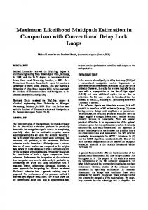
Then, the LL function can be rewritten as (37) Fig. 1. Sparse nonuniform array and equivalent ULA used in simulations. (a) Sparse array. (b) ULA.

where Re

Im

(38)

is the vector of unknown real parameters, and . It can be readily verified that the result of (22) remains valid in by in the uncalibrated array case if we replace this equation. Similarly, the results of (26) and (31) remain valid by . Note that now the LL function (31) if we replace . also depends on , i.e., In order to find the ML estimate of the vector , we rewrite the LL function (37) as

subarrays of four, three, and two sensors, respectively. Each interelement spacing. The first of these subarrays has the apart from each other, and second subarrays are spaced apart from while the second and third subarrays are spaced each other. The configuration of the array is shown in Fig. 1(a). Throughout all examples, we assume that the noises between all three subarrays are uncorrelated and that the noise covariance matrix has the following block-diagonal form bdiag where , and respectively, and

are the 4

(41) 4, 3

3, and 2

2 matrices,

tr (39)

(42)

and setDifferentiating (39) with respect to ting the result to zero, we obtain the following system of linear equations:

The values , and are assumed. Note that the covariance model in (42) has found numerous applications in sonar and wireless communications (see [16], [30]–[33], and references therein). The method of [17] is based on the assumption that the array is a ULA. Therefore, to enable comparison with this method, sensors and we test it using an “equivalent” ULA with spacing, which has the same aperture as the nonuniform array used. The configuration of this equivalent ULA is shown in Fig. 1(b). Note that using such an equivalent array instead of the nonuniform array of Fig. 1(a), we favor the method of [17] with respect to the other methods tested because the equivalent ULA of Fig. 1(b) has more sensors than the nonuniform array of Fig. 1(a). The noise covariance matrix for the equivalent ULA is assumed to have the following form:

(40) and stands for the complex conjugate. where By fixing , and , and solving the system (40) for , we can find the ML estimate for the latter parameter. Similar to the calibrated array case considered in the previous section, the ML DOA estimator can be formulated as an iterative procedure. Note that in Step 1, in addition to the initialization as . Moreover, an of , we also should initialize additional step after Step 3 is required. In this step, the matrix is estimated by solving the system of linear equations in (40) with fixed , and that have been estimated in the previous steps. In Appendix B, we derive the deterministic CRB for the uncalibrated array case using the model (36) parameterized by means of the vector (38). V. SIMULATIONS In this section, we numerically compare the performance of the proposed ML DOA estimator with that of the ML colored noise modeling-based technique by Friedlander and Weiss [10] and the approximate technique by Agrawal and Prasad [17], as well as with the deterministic and stochastic CRBs in the colored noise case (see [9] and [16]). For the proposed method and the method of [10], we assume a sparse linear array of sensors with the aperture of , where is the wavelength. This array is assumed to consist of three uniform linear

bdiag

(43)

Throughout all simulation examples, we assume two narrowband far-field signal sources of equal power impinging on the array from and relative to the broadside. The complex-valued signal waveforms are modeled as zero-mean temporally white Gaussian processes. The root-mean-square errors (RMSEs) of DOA estimation are displayed in Figs. 2–6, and each point is obtained using 100 independent simulation runs. A genetic algorithm is used to optimize the ML-based criteria in all the techniques tested. The parameters of the genetic algorithm (e.g., see [34]) were optimized to ensure its convergence to the global maximum. Two iterations of our ML algorithm given in Section III-B are used to obtain the final DOA estimates. For the Friedlander–Weiss algorithm, six real-valued nuisance noise parameters are employed to model the noise field. Therefore, the dimension of the parameter space (and, correspondingly, the


39

Fig. 2. DOA estimation RMSEs and CRBs versus the number of snapshots. Uncorrelated sources.

Fig. 4. DOA estimation RMSEs and CRBs versus the number of snapshots. Correlated sources.

Fig. 3. DOA estimation RMSEs and CRBs versus the SNR. Uncorrelated sources.

Fig. 5. DOA estimation RMSEs and CRBs versus the SNR. Correlated sources.

computational burden) of the latter algorithm is much higher than that of our method. In the first example, we assume uncorrelated sources with the dB, where, similar to [12] and [18] SNR

In our fourth example, we assume correlated sources again, is taken. The performances of the methods tested and are shown in Fig. 5 versus the SNR. In the fifth example, the array gains and phases are assumed to be unknown, i.e., the model (36) is applied, where diag . The unknown non-negative are independently drawn in each simulation gains run from a uniform random generator with the standard deviare ation equal to one, while the unknown phases . independently and uniformly drawn from the interval dB, and the results In this example, we assume that SNR are displayed in Fig. 6 versus the number of snapshots. From Figs. 2–6, we observe that the proposed method consistently outperforms the Agrawal–Prasad and Friedlander–Weiss techniques and that two iterations of our algorithm are sufficient to converge in performance to the corresponding CRBs. These improvements can be explained by the fact that our technique explicitly uses the block-diagonal structure of the noise

SNR

(44)

being the signal power. Fig. 2 shows the RMSEs of with the DOA estimates for the methods tested versus the number of snapshots. In the second example, we assume uncorrelated sources again . Fig. 3 displays the DOA estimation RMSEs of and the same methods versus the SNR. In the third example, mutually correlated sources are assumed with the correlation coefficient equal to 0.9. In this example, we dB, and the results are displayed in Fig. 4 assume that SNR versus the number of snapshots.

40


APPENDIX A PROOF OF (24) The matrix

can be rewritten as bdiag

(45)

where is the th block on the main diagonal of that is selected by the corresponding th block of . Partitioning the matrix as

.. .

.. .

..

.

(46)

.. .

and using the property Fig. 6. DOA estimation RMSEs and CRBs versus the number of snapshots. Unknown array gains and phases.

covariance matrix, whereas the Agrawal–Prasad and Friedlander–Weiss methods do not exploit this structure. In particular, from Figs. 3 and 5 it can be seen that the proposed method has approximately 2.5 dB of improvement with respect to the Friedlander–Weiss algorithm. The Agrawal–Prasad method performs much worse than the other two methods in all examples. In the last example, the performance of the Friedlander–Weiss method becomes very poor because it does not include unknown gains and phases in the model parameters. The proposed algorithm with estimation of unknown gains and phases performs reasonably close to the CRB in the latter case.

bdiag

(47)

we have

.. .

.. .

..

.

.. . (48)

where

is the

identity matrix. From (48), it follows that

(49)

tr

Using (49) and the properties of the trace operator, we can rewrite the second term in the right-hand side of (23) as VI. CONCLUSION We have addressed the problem of ML DOA estimation in unknown spatially correlated noise fields using sparse sensor arrays composed of multiple widely separated subarrays. A new deterministic ML DOA estimator has been derived for the considered class of sparse sensor arrays. The proposed approach concentrates the criterion of the estimation problem with respect to all nuisance parameters. In contrast to the analytic concentration used in the conventional ML techniques, the implementation of the proposed technique is based on an iterative procedure, which includes a stepwise concentration of the LL function. The extension of the proposed technique to the case of uncalibrated arrays has also been developed and the deterministic DOA estimation CRB has been derived for this case. Computer simulations have shown that our algorithm requires only a few steps to converge in performance to the corresponding CRB. They also have demonstrated essential performance improvements achieved by the proposed technique relative to the popular ML techniques by Agrawal and Prasad and by Friedlander and Weiss, which do not take any advantage of the array sparsity.

tr tr tr (50) and this proves (24). APPENDIX B DERIVATION OF THE DETERMINISTIC CRB IN THE CASE OF UNCALIBRATED ARRAY In the deterministic case, the elements of the Fisher information matrix (FIM) are given by [18] tr Re

(51)


where the

41

vector

Re

Re

(52)

Re

are the elements of the parameter vector given by (38), stands for the Kronecker matrix product, and the size of the . identity matrix is The derivatives of with respect to different parameters are given by

(67) Im

Im Im (68)

(53)

Re

Re

(54)

Re

(55)

Im

Im Re Im

Im Re Im

Re (69)

Re (56)

Re

Im

Im (57) has the dimensions where the vector (54)–(55) and (56)–(57), respectively, and

and

Im Re Re Im Im Re Im

in

(70) (71)

(58) diag

(59)

Using (53)–(57), the submatrices of the FIM are given by

where is the Kronecker delta, and the vector has the dimension . Note that all the FIM cross-terms involving the signal and noise parameters have zero values. Let us introduce the block-diagonal matrix

Re (60) Re

Re

Re

Im Re

Re

Im Re

..

(72)

.

Im (61)

Im Im Im

where the matrices

are defined as

Re Re Im

(62) Im

Re Re

Re Im

Im Im

(73)

and denote

Re

.. .

..

.. .

.

(74)

(63) Re

Im

Im

Re

where the matrices

Im (64) Re Im

Re Re Im Im

are defined as

Re Re Re Im Re Im In addition, let us introduce the matrices

Im Im

(75)

(76) (65)

(77) (78)

(66)

(79)

42


.. .

..

.

.. .

(80)

.. .

..

.. .

(81)

.

where the matrices ; and are defined as Re Re Re Re Re Im Re Im

(82)

Im Im

(83)

Im

(84) (85)

Im Re Re Re Re

Re Im Re Im

Im Im Im Im

(86) (87)

Using this notation, the FIM can be written as

(88)

Using the partitioned matrix inversion formula, the matrix that corresponds to the unknown parameters written as CRB

CRB can be

(89)

where (90) (91)

REFERENCES [1] Y. Bresler and A. Macovski, “Exact maximum likelihood parameter estimation of superimposed exponential signals in noise,” IEEE Trans. Acoust., Speech, Signal Process., vol. ASSP-34, no. 10, pp. 1081–1089, Oct. 1986. [2] J. F. Böhme, “Estimation of spectral parameters of correlated signals in wavefields,” Signal Process., vol. 10, pp. 329–337, 1986. [3] I. Ziskind and M. Wax, “Maximum likelihood localization of multiple sources by alternative projection,” IEEE Trans. Acoust., Speech, Signal Process., vol. 36, no. 10, pp. 1553–1560, Oct. 1988. [4] P. Stoica and A. Nehorai, “MUSIC, maximum likelihood and Cramér-Rao bound,” IEEE Trans. Acoust., Speech, Signal Process., vol. 37, no. 5, pp. 720–741, May 1989. [5] , “Performance study of conditional and unconditional direction-ofarrival estimation,” IEEE Trans. Acoust., Speech, Signal Process., vol. 38, no. 10, pp. 1783–1795, Oct. 1990. [6] , “On the concentrated stochastic likelihood function in array signal processing,” Circuits, Syst., Signal Process., vol. 14, no. 9, pp. 669–674, Sep. 1995.

[7] K. M. Wong, J. P. Reilly, Q. Wu, and S. Qiao, “Estimation of the directions of arrival of signals in unknown correlated noise. Part I: The MAP approach and its implementation,” IEEE Trans. Signal Process., vol. 40, no. 8, pp. 2007–2017, Aug. 1992. [8] J. LeCadre, “Parametric methods for spatial signal processing in the presence of unknown colored noise field,” IEEE Trans. Acoust., Speech, Signal Process., vol. 37, no. 7, pp. 965–983, Jul. 1989. [9] H. Ye and R. D. DeGroat, “Maximum likelihood DOA estimation and asymptotic Cramér-Rao bounds for additive unknown colored noise,” IEEE Trans. Signal Process., vol. 43, no. 4, pp. 938–949, Apr. 1995. [10] B. Friedlander and A. J. Weiss, “Direction finding using noise covariance modeling,” IEEE Trans. Signal Process., vol. 43, no. 7, pp. 1557–1567, Jul. 1995. [11] B. Göransson and B. Ottersten, “Direction estimation in partially unknown noise fields,” IEEE Trans. Signal Process., vol. 47, no. 9, pp. 2375–2385, Sep. 1999. [12] A. B. Gershman, A. L. Matveyev, and J. F. Böhme, “Maximum likelihood estimation of signal power in sensor array in the presence of unknown noise field,” Proc. INstg. Elect. Eng. Radar, Sonar, Navigation, vol. 142, no. 5, pp. 218–224, Oct. 1995. [13] M. Viberg, P. Stoica, and B. Ottersten, “Array processing in correlated noise fields based on instrumental variables and subspace fitting,” IEEE Trans. Signal Process., vol. 43, no. 5, pp. 1187–1199, May 1995. , “Maximum likelihood array processing in spatially correlated [14] noise fields using parameterized signals,” IEEE Trans. Signal Process., vol. 45, no. 4, pp. 996–1004, Apr. 1997. [15] P. Stoica, M. Viberg, K. M. Wong, and Q. Wu, “Maximum-likelihood bearing estimation with partly calibrated arrays in spatially correlated noise field,” IEEE Trans. Signal Process., vol. 44, no. 4, pp. 888–899, Apr. 1996. [16] A. B. Gershman, P. Stoica, M. Pesavento, and E. Larsson, “The stochastic Cramér-Rao bound for direction estimation in unknown noise fields,” Proc. Inst. Elect. Eng. Radar, Sonar, Navigat., vol. 149, no. 1, pp. 2–8, Feb. 2002. [17] M. Agrawal and S. Prasad, “A modified likelihood function approach to DOA estimation in the presence of unknown spatially correlated Gaussian noise using a uniform linear array,” IEEE Trans. Signal Process., vol. 48, no. 10, pp. 2743–2749, Oct. 2000. [18] M. Pesavento and A. B. Gershman, “Maximum-likelihood direction of arrival estimation in the presence of unknown nonuniform noise,” IEEE Trans. Signal Process., vol. 49, no. 7, pp. 1310–1324, Jul. 2001. [19] Q. Wu and K. M. Wong, “UN-MUSIC and UN-CLE: An application of generalized correlation analysis to the estimation of the directions of arrival of signals in unknown correlated noise,” IEEE Trans. Signal Process., vol. 42, no. 9, pp. 2331–2343, Sep. 1994. , “Estimation of DOA in unknown noise: Performance analysis of [20] UN-MUSIC and UN-CLE, and the optimality of CCD,” IEEE Trans. Signal Process., vol. 43, no. 2, pp. 454–468, Feb. 1995. [21] M. D. Zoltowski and K. T. Wong, “Closed-form eigenstructure-based direction finding using arbitrary but identical subarrays on a sparse uniform Cartesian array grid,” IEEE Trans. Signal Process., vol. 48, no. 8, pp. 2205–2210, Aug. 2000. [22] A. L. Swindlehurst, P. Stoica, and M. Jansson, “Exploiting arrays with multiple invariances using MUSIC and MODE,” IEEE Trans. Signal Process., vol. 49, no. 11, pp. 2511–2521, Nov. 2001. [23] M. Pesavento, A. B. Gershman, and K. M. Wong, “Direction of arrival estimation in partly calibrated time-varying sensor arrays,” in Proc. Int. Conf. Acoust., Speech, Signal Process., Salt Lake City, UT, May 2001, pp. 3005–3008. [24] , “Direction finding in partly calibrated sensor arrays composed of multiple subarrays,” IEEE Trans. Signal Process., vol. 50, no. 9, pp. 2103–2115, Sep. 2002. [25] , “On uniqueness of direction of arrival estimates using rank reduction estimator (RARE),” in Proc. Int. Conf. Acoust., Speech, Signal Process., Orlando, FL, May 2002. [26] C. M. S. See and A. B. Gershman, “Direction-of-arrival estimation in partly calibrated subarray-based sensor arrays,” IEEE Trans. Signal Process., vol. 52, no. 2, pp. 329–338, Feb. 2004. [27] A. B. Gershman, “Robustness issues in adaptive beamforming and high-resolution direction finding,” in High-Resolution and Robust Signal Processing, Y. Hua, A. B. Gershman, and Q. Cheng, Eds. New York: Marcel Dekker, 2003, pp. 63–110. [28] J. P. Burg, D. G. Luenberger, and D. L. Wenger, “Estimation of structured covariance matrices,” Proc. IEEE, vol. 70, no. 9, pp. 963–974, Sep. 1982.


[29] D. Astléy, A. L. Swindlehurst, and B. Ottersten, “Spatial signature estimation for uniform linear arrays with unknown recever gain and phases,” IEEE Trans. Signal Process., vol. 47, no. 8, pp. 2128–2138, Aug. 1999. [30] A. Paulraj and T. Kailath, “Direction of arrival estimation by eigenstructure methods with imperfect spatial coherence of wave fronts,” J. Acoust. Soc. Amer., vol. 83, no. 3, pp. 1034–1040, Mar. 1988. [31] T. Trump and B. Ottersten, “Estimation of nominal direction of arrival and angular spread using an array of sensors,” Signal Process., vol. 50, no. 4, pp. 57–70, Apr. 1996. [32] A. B. Gershman, C. F. Mecklenbräuker, and J. F. Böhme, “Matrix fitting approach to direction of arrival estimation with imperfect spatial coherence of wavefronts,” IEEE Trans. Signal Process., vol. 45, no. 7, pp. 1894–1899, Jul. 1997. [33] O. Besson, F. Vincent, P. Stoica, and A. B. Gershman, “Approximate maximum likelihood estimators for array processing in multiplicative noise environments,” IEEE Trans. Signal Process., vol. 48, no. 9, pp. 2506–2518, Sep. 2000. [34] A. B. Gershman and P. Stoica, “Direction finding using data-supported optimization,” Circuits, Syst., Signal Process., vol. 20, no. 5, pp. 541–549, Oct. 2001.

Sergiy A. Vorobyov (M’02) was born in Ukraine in 1972. He received the M.S. and Ph.D. degrees in systems and control from Kharkiv National University of Radioelectronics (KNUR), Kharkiv, Ukraine, in 1994 and 1997, respectively. From 1995 to 2000, he was with the Control and Systems Research Laboratory at KNUR, where he became a Senior Research Scientist in 1999. From 1999 to 2001, he was with the Brain Science Institute, RIKEN, Tokyo, Japan, as a Research Scientist. From 2001 to 2003, he was with the Department of Electrical and Computer Engineering, McMaster University, Hamilton, ON, Canada, as a Postdoctoral Fellow. Since 2003, he has been a Research Fellow with the Department of Communication Systems, University of Duisburg-Essen, Duisburg, Germany. He also held short-time visiting appointments at the Institute of Applied Computer Science, Karlsruhe, Germany, and Gerhard-Mercator University, Duisburg. His research interests include control theory, statistical array signal processing, blind source separation, robust adaptive beamforming, and wireless and multicarrier communications. Dr. Vorobyov was a recipient of the 1996–1998 Young Scientist Fellowship of the Ukrainian Cabinet of Ministers, the 1996 and 1997 Young Scientist Research Grants from the George Soros Foundation, and the 1999 DAAD Fellowship (Germany).

Alex B. Gershman (M’97–SM’98) received the Diploma (M.Sc.) and Ph.D. degrees in radiophysics from the Nizhny Novgorod State University, Nizhny Novgorod, Russia, in 1984 and 1990, respectively. From 1984 to 1989, he was with the Radiotechnical and Radiophysical Institutes, Nizhny Novgorod. From 1989 to 1997, he was with the Institute of Applied Physics, Russian Academy of Science, Nizhny Novgorod, as a Senior Research Scientist. From the summer of 1994 until the beginning of 1995, he was a Visiting Research Fellow at the Swiss Federal Institute of Technology, Lausanne, Switzerland. From 1995 to 1997, he was Alexander von Humboldt Fellow at Ruhr University, Bochum, Germany. From 1997 to 1999, he was a Research Associate at the Department of Electrical Engineering, Ruhr University. In 1999, he joined the Department of Electrical and Computer Engineering, McMaster University, Hamilton, ON, Canada where he is now a Professor. Currently, he also holds a visiting professorship at the Department of Communication Systems, University of Duisburg-Essen, Duisburg, Germany. His research interests are in the area of signal processing and communications, and include statistical and array signal processing, adaptive beamforming, spatial diversity in wireless communications, multiuser and MIMO communications, parameter estimation and detection, and spectral analysis. He has published over 220 technical papers in these areas.

43

Dr. Gershman was a recipient of the 1993 International Union of Radio Science (URSI) Young Scientist Award, the 1994 Outstanding Young Scientist Presidential Fellowship (Russia), the 1994 Swiss Academy of Engineering Science and Branco Weiss Fellowships (Switzerland), and the 1995-1996 Alexander von Humboldt Fellowship (Germany). He received the 2000 Premier’s Research Excellence Award of Ontario and the 2001 Wolfgang Paul Award from the Alexander von Humboldt Foundation, Germany. He is also a recipient of the 2002 Young Explorers Prize from the Canadian Institute for Advanced Research (CIAR), which has honored Canada’s top 20 researchers 40 years of age or under. He is an Associate Editor of the IEEE TRANSACTIONS ON SIGNAL PROCESSING and the EURASIP Journal on Wireless Communications and Networking and a Member of the Sensor Array and Multichannel Signal Processing Technical Committee of the IEEE Signal Processing Society. He was Technical Co-Chair of the Third IEEE International Symposium on Signal Processing and Information Technology, Darmstadt, Germany, in December 2003. He is Technical Co-Chair of the Fourth IEEE Workshop on Sensor Array and Multichannel Signal Processing, to be held in Waltham, MA, in July 2006.

Kon Max Wong (F’02) was born in Macau. He received the B.Sc.(Eng), D.I.C., Ph.D., and D.Sc.(Eng) degrees, all in electrical engineering, from the University of London, London, U.K., in 1969, 1972, 1974, and 1995, respectively. He was with the Transmission Division of Plessey Telecommunications Research Ltd., London, in 1969. In October 1970, he was on leave from Plessey, pursuing postgraduate studies and research at Imperial College of Science and Technology, London. In 1972, he rejoined Plessey as a research engineer and worked on digital signal processing and signal transmission. In 1976, he joined the Department of Electrical Engineering, Technical University of Nova Scotia, Halifax, NS, Canada, and in 1981, he moved to McMaster University, Hamilton, ON, Canada, where he has been a Professor since 1985 and served as Chairman of the Department of Electrical and Computer Engineering from 1986 to 1987 and again from 1988 to 1994. He was on leave as a Visiting Professor at the Department of Electronic Engineering, the Chinese University of Hong Kong, from 1997 to 1999. At present, he holds the title of NSERC-Mitel Professor of Signal Processing and is the Director of the Communication Technology Research Centre at McMaster University. His research interest is in signal processing and communication theory, and he has published over 170 papers in the area. Prof. Wong was the recipient of the IEE Overseas Premium for the best paper in 1989, is a Fellow of the Institution of Electrical Engineers, a Fellow of the Royal Statistical Society, and a Fellow of the Institute of Physics. He also served as an Associate Editor of the IEEE TRANSACTION ON SIGNAL PROCESSING from 1996 to 1998 and has been the chairman of the Sensor Array and Multichannel Signal Processing Technical Committee of the Signal Processing Society since 1998. He received a medal presented by the International Biographical Centre, Cambridge, U.K., for his “outstanding contributions to the research and education in signal processing” in May 2000 and was honored with the inclusion of his biography in the books Outstanding People of the 20th Century and 2000 Outstanding Intellectuals of the 20th Century, which were published by IBC to celebrate the arrival of the new millennium.