2003 Conference on Information Sciences and Systems, The Johns Hopkins University, March 12–14, 2003
Maximum Likelihood Estimation of Internal Network Link Delay Distributions Using Multicast Measurements E. Lawrence1 , G. Michailidis2 , and V. N. Nair3 Department of Statistics The University of Michigan Ann Arbor, MI 48109 Abstract — There is increased interest among network administrators and service providers to estimate quality of service parameters associated with their network operations. Two approaches are currently used for collecting and modeling network data: passive monitoring of link-level data or active probing to obtain path-level measurements. In this paper, we investigate the estimation of link delay distributions based on active network tomography based on information gathered from end-to-end multicast measurements. We derive the maximum likelihood estimator, establish its asymptotic properties, and investigate its finitesample performance. Comparisons with a heuristic estimation scheme proposed in the literature are also made.
I. I NTRODUCTION Background: Modern computer and communications networks have evolved into large and complex systems that are decentralized and loosely controlled. As a result, it has become increasingly difficult to monitor and assess their performance and determine quality of service. Nevertheless, providers are constantly seeking ways to monitor their network with regard to characteristics such as traffic intensity, delay, loss, dropped packets, etc. in order to ensure high quality of service to users. Additionally, the networks are often vulnerable to malicious attacks, for example distributed denial of service (DDoS) attacks in which many attacker sites send messages to a victim site in order to disable it. As an example, consider the recent Code Red virus [11] which coopts personal computers as ’zombies’ and uses them to conduct DDoS attacks. There is a critical need for techniques to detect and locate these attacks, particularly as they become more widespread and powerful. While it may be fairly simple for a provider to investigate problems within his own domain, detecting and locating problems that arise in other portions of the Internet is not nearly as easy. Traditional queuing and traffic models are not adequate for capturing the overall behavior of these complex networks. Currently, there are two basic approaches that have been found useful for studying and characterizing network performance: active and passive monitoring. Passive traffic measurement involves capturing packets as they are sent across links and collecting information about them. This information is usually collected at the link level and used to estimate path-level characteristics. Active probing, on the other hand, involves sending probes across a network and keeping track of information such as numbers of packets sent and received and the length of time it takes packets to travel from a root node to the receiver node. This information is then used to estimate internal link-level parameters from the end-to-end path-level measurements. 1 Corresponding 2 The
author:
[email protected] work of G. Michailidis was partially supported by NSF grant IIS
9988095. 3 The work of V. N. Nair was was partially supported by NSF grant DMS 0204247.
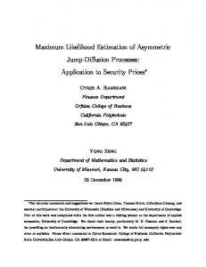
Both of these schemes require estimation of network performance parameters from a limited set of link-level or path-level measurements. Vardi [1] introduced the term network tomography to describe this class of estimation problems. His paper considered the estimation of source-destination traffic intensity along links in a network based on measurements of traffic flow on directed links. There has been considerable work in this area recently, covering many aspects of the network tomography problem. In this paper, we focus on estimating internal link-level parameters (specifically delay distributions) from multicast probing schemes (to be described below). Past work on this problem is reviewed in Section 1.3. For an excellent up-to-date review of the state of network tomography, readers are referred to Coates, Hero, Nowak, and Yu [2]. Framework and Notation: Networks can typically be captured by graphs with nodes representing computers or routers and edges representing the links between them. The objective is to monitor the network’s activity by relying on measurements obtained from a limited number of nodes usually located at the periphery of the network, where access is easy. The monitoring scheme relies on active probing of the network, with packets sent from a source node to a set of destination nodes where the end-to-end (source-destination) delays are recorded. The time delays are additive across links and consist of both propagation (latency) delays and router processing (queuing) delays along the path. In this paper we focus on multicast transmissions: at internal routing nodes where forking occurs (see node 1 in Figure 1), each packet is replicated and sent along each branching path. So the packet is effectively sent from the root node to all of the receiver nodes. The key to multicast transmissions for network tomography is that it introduces dependencies between end-to-end delays measured by different receivers, which in turn enables inferences about network internal links characteristics. We will restrict attention to networks whose topologies can be represented by trees whose regularity renders the inference problem computationally tractable. Next, we introduce the necessary definitions and notation. Refer to Figure 1 throughout for a concrete graphical representation. Let T = (V, E ) denote a tree with node set V and link (edge) set E . The nodes will all be denoted by a number and each link will be named after the node at its terminus. Let {0} ∈ V denote the root node from which all multicast packets originate. Let R denote the set of receiver nodes. The parent of node k ∈ V will be denoted by f (k). Note that all nodes, except the root node, have a parent node. Let the function f i (k) be defined in the following recursive manner: f i (k) = f (f i−1 (k)) with f 1 (k) = f (k). All nodes in V − R have a set of child nodes, with the set of children of node k denoted by d(k). A node k is said to be in level L = 1, 2, . . . if f L (k) = 0. The deepest level of the tree will be denoted by L. The trees that we study in this paper are assumed to be binary and symmetric. Thus, all of the nodes except the root node and receiver nodes have exactly two children, and all nodes in R (receiver nodes) are in level L (level of the tree).
0
0 (root node)
1
L=1
1 f(4)=f(5)=2
4
3
5
6
L=2
7
L=3 R
d(2) Figure 1: An example of a tree topology with some of the notation used illustrated We will assume the following framework for the data collection, modeling, and inference. (This formulation is common to most of the other papers in the literature as well.) The delay distribution for each link will be assumed to be discrete, and we will estimate it nonparametrically. Let the delay accumulated on each link k be denoted by Xk . Then, Xk will take values in the set {0, q, 2q, . . . , bq} where q is the unit of measurement and b is an integer that defines the maximum delay for each link. It is assumed throughout that the values of q and b are common to all link delay distributions. Also, for the sake of simplicity, we will not consider in this paper the possibility that Xk could be infinite, which corresponds to the case where the packets are dropped or lost along their path. This extension can be handled easily and will be addressed in future work. We will consider inference under the stochastic assumption that the individual link delays Xk are mutually independent. (This assumption is common in the current literature. Extensions to spatial and temporal dependence will be studied in future work). Let αk (i) = P {Xk = iq}, i = 1, . . . , b and k ∈ V. In the rest of the paper, for notational convenience, we will drop the use of the universal measurement unit q. Further, we will denote by α ~ k = (αk (1), αk (2), . . . , αk (b))0 , a column vector containing all of the link k delay probabilities. Let α ~ = {~ αk , k ∈ V}, a column vector containing all the parameters of interest that have to be estimated. Let Yk denote the accumulated delay at node k. For example, in Figure 1, Y3 = X1 + X3 and Y5 = X1 + X2 + X5 . Only the accumulated (end-to-end) delays at the receiver nodes are recorded; ~ = {Yj ; j ∈ R}. Note that for j ∈ R, i.e., we observe only Y Yj ∈ {0, ..., Lb} where L is the number of layers in the tree. Each multicast probe packet experiences a delay on each link along its path. Let X = {0, 1, . . . , b}|E| be the space of all possible link delays. Hence, ~ x ∈ X is an |E|-tuple describing the individual link delays that the probe experienced. Let ~ y (~ x) be the multicast end-to-end measurement that results when ~ x occurs. Note that this is a manyto-one function; there are several ~ x outcomes that result in the same ~ y. Denote by Y = {~ y (~ x); ~ x ∈ X } the space of all possible multicast results. Let us consider an example on the two-layer tree shown in Fig-
3
2 Figure 2: Two-Layer Tree
ure 2. Let b = 1, so Xk ∈ {0, 1}. Suppose that a probe experiences delays of 1, 0 and 1 on links 1, 2, and 3, respectively. Then, ~ x = (1, 0, 1) and the observed set of end-to-end delays at receivers 1 and 2 would be ~ y=~ y (~ x) = (1, 2). For this tree, the entire set of individual link outcomes is given by X = {(0, 0, 0), (0, 0, 1), (0, 1, 0), (0, 1, 1), (1, 0, 0),
(1)
(1, 0, 1), (1, 1, 0), (1, 1, 1)},
while the set of observable outcomes is given by Y = {(0, 0), (0, 1), (1, 0), (1, 1), (1, 2), (2, 1), (2, 2)}.
(2)
~ = {Xk ; k ∈ V} represent the collection of all Let the variable X individual link delays. The probability of the above outcome is given by ~ = (1, 0, 1)} = α1 (1)α2 (0)α3 (1), P {X (3) and the probability of the observed end-to-end delay by ~ = (1, 2)} = α1 (0)α2 (1)α3 (2) + α1 (1)α2 (0)α3 (1) P {Y
(4)
because there are two sets of link delays that give rise to this particular end-to-end delay pair. Literature Review: There have been several papers recently on the estimation of link-level parameters based on end-to-end path-level measurements. They consider both unicast and multicast measurement schemes. Unicast refers to a transmission scheme where the root node sends (separate) packets, one at a time, to the receiver nodes. Unicast schemes suffer from identifiability problems, and there have been modifications such as back-to-back unicast that have been proposed [2]. We consider only multicast schemes here. The primary focus on past work has been on estimating link-level loss rates and delays. Link loss refers to the probability of dropping or losing packets of information due primarily to buffer overflows at router nodes along a link. The multicast link loss problem was studied in C´aceres, Duffield, Horowitz, and Towsley [8]. They devised a clever method to compute the maximum likelihood estimates (MLEs) under the assumption of spatial and temporal independence. However, the computation of the variance-covariance matrix and associated inference is complicated. A computationally simpler approach based
on various least-squares methods with superior performance in small samples is considered in Xi, Michailidis, and Nair [14]. In a recent paper, Shih and Hero [9] have considered link delay estimation based on unicast probing schemes. This paper assumes that the link delay distributions are a mixture of Gaussian distributions and a point mass at zero. They discuss the identifiability problem associated with unicast schemes and present a sufficient condition for identifiability. However, checking whether this condition holds in real applications remains an open issue. Lo Presti, Duffield, Horowitz, and Towsley (hereafter referred to as LDHT) [6] was the first paper to investigate inference for linklevel delay distributions based on multicast probing schemes. It considers nonparametric estimation for discrete delay distributions under the framework in Section 1.2. Although the estimation method in LDHT mirrors the MLE approach for link loss probabilities in C´aceres et al. [8], it does not lead to MLEs for the delay distributions. We describe it in some detail below since we will be comparing the efficiency of their method with the maximum likelihood estimator (MLE) later in the paper. We need some additional notation. Let Ak (i) = P {Yk = i}, the probability that the cumulative delay at node k is equal to i. Let T (k) = (V(k), E (k)) be the subtree with root node k (but connected to the root node 0), and let R(k) be the receiver set of this tree. Let γk (i) = P {minj∈R(k) Yj ≤ i}, the probability that the minimum end-to-end delay measured in the subtree T (k) is less than or equal to i. Finally, let βk (i) = P {minj∈R(k) Yj −Yf (k) ≤ i}, the probability that the minimum delay experienced on the subtree T (k) is less than i. Note the difference between γk (i) and βk (i). The former is the total end-to-end delay starting from node 0 while the latter is the delay accumulated only within the subtree starting at node k. For node k ∈ R, there is a simple relationship between γk (i) and Ak (i): Ak (0) = γk (0), (5) and for i > 0, Ak (i) = γk (i) −
i−1 X
Ak (j).
(6)
j=0
For a node k not in the receiver set, LDHT show that the Ak (i) can be represented as solutions of polynomial equations of order d(k), the number of direct descendants of k, involving the γk ’s and the βk ’s. The βk ’s themselves can be expressed in terms of the γk ’s and Ak ’s. Finally, αk (i) can be expressed in terms of Ak (j), Af (k) (j) for j = 1, . . . , i and αk (j) for j < i. In summary, all of the expressions depend only on the γk ’s. The estimation method in LDHT is based on substituting the following empirical estimators of the γk ’s γˆk (i) =
n 1 X ˆ I{Yk,m ≤ i}, n
(7)
m=1
where Yˆk,m = minj∈R(k) Yˆj,m , (the Yˆj,m j ∈ R(k) are the end-toend delays in subtree T (k) from probe m) and solving the polynoˆk ’s and then for βˆk ’s and α mial equations for A ˆ k ’s. The interested reader should refer to [6] for details. It is worth noting that this solution allows for infinite delays and unbalanced tree topologies. LDHT shows that the estimators are consistent and asymptotically normal. Although the solution is non-iterative, it is still cumbersome to implement. One has to solve complicated polynomials: b polynomials of degree d(k) for every node k. Additionally, for small numbers of probes, the appropriate solution to these polynomials may not even be positive. The second problem is the loss of information. The solution uses only the empirical quantities γ ˆk (i), i = 0, . . . , (b − 1),
the end-to-end delays that are smaller than the maximum link delay. Information from the end-to-end delays between b and Lb − 1 is ignored. Discarding this information leads to considerable inefficiency, which increases as the tree and bin sizes grow larger. We do a limited efficiency comparison with the MLE in Section III. Furthermore, the variance-covariance matrix of this estimator is difficult to compute except in small trees. This severely limits the ability to develop inference procedures.
II. M AXIMUM L IKELIHOOD E STIMATION OF THE D ISCRETE L INK D ELAY D ISTRIBUTION In this section, we develop the nonparametric MLE of the delay distribution and describe the expectation-maximization (EM) algorithm [13] for computing the MLE. Let N~y be the number of probes that resulted in outcome ~ y ∈ Y. ~ = ~ Let g(~ y; α ~ ) = P {Y y }. Then, the observed data correspond to a multinomial experiment in terms of the observed end-to-end link delays, and the log-likelihood can be expressed as l(~ α) =
X
N~y log[g(~ y; α ~ )].
(8)
~ y ∈Y
This likelihood is a complicated function of the α’s and is difficult to maximize directly. The problem arises from the fact that we observe only the end-to-end delays. If the unobserved individual link delays were available, the estimation problem is straightforward. The EM algorithm is a natural approach for computing the MLEs in this kind of missing data problem. It is an iterative algorithm that starts with some initial estimate of the desired parameter values. The missing data (or the sufficient statistics) are imputed using these estimates. The ”complete data” (observed data supplemented with the imputed missing data) are then used to obtain new estimates of the parameter values. The process is repeated until the likelihood converges to a maximum. Each step of the algorithm is guaranteed to increase the likelihood, so the solution will converge to a local maximum or stationary point [12]. Let M~x be the number of times that a particular individual link delay set occurred. This is a sufficient statistic of our missing data. If we knew these values, the parameter estimation would be quite simple. These are missing however, but we can impute them as follows. Given an estimate of α ~ , we impute the M~x from the N~y . With these imputed values, we can calculate new estimates of the α ~ and repeat the process. Formally, let the q-th step estimate of the delay distribution of all the links in the tree topology be denoted by α ~ (q) . Using this estimate, (q) ~ (q) ~ we can compute P {X = ~ x} and P {Y = ~ y (~ x)}. With these values, we can now impute the required quantities in the E-step: (q+1)
M~x
= N~y
~ =~ P (q) {X x} . (q) ~ P {Y = ~ y(~ x)}
(9)
If we let Xk,i = {~ x ∈ X |xk = i}, then the M-step is (q+1)
αk
(i) =
1 X (q+1) M~x . n
(10)
~ x∈Xk,i
Notice that in many cases these calculations simplify, since some outcomes ~ y can only arise from a single ~ x; in such a case the probability ratio in (9) will just be 1. For example, this occurs when ~ y = ~0 in which case ~ x = ~0. Example: To illustrate the process concretely, consider the following example of a two-layer tree with maximum link delay b = 2. Starting from an estimate α ~ (q) , here are the steps needed to produce
(q+1)
5
α1 (0). First we impute the necessary sufficient statistics in the E-step.
−6.06
−6.07
=
N0,0
−6.08
M0,0,1
(q+1)
=
N0,1
−6.09
(q+1) M0,0,2
=
N0,2
(q+1) M0,1,0
=
N1,0
(q+1)
=
M0,1,1
(q+1)
M0,1,2
(q+1)
M0,2,0
(q+1)
M0,2,1
(q+1)
M0,2,2
= = = =
Log−Likelihood
(q+1)
M0,0,0
x 10
−6.1
−6.11
(q) (q) (q) α1 (0)α2 (1)α3 (1)N1,1 (q) (q) (q) (q) (q) (q) α1 (0)α2 (1)α3 (1) + α1 (1)α2 (0)α3 (0) (q) (q) (q) α1 (0)α2 (1)α3 (2)N1,2 (q) (q) (q) (q) (q) (q) α1 (0)α2 (1)α3 (2) + α1 (1)α2 (0)α3 (1)
N2,0 (q) (q) (q) α1 (0)α2 (2)α3 (1)N2,1 (q) (q) (q) (q) (q) (q) α1 (0)α2 (2)α3 (1) + α1 (1)α2 (1)α3 (0) (q) (q) (q) α1 (0)α2 (2)α3 (2)N2,2 2 (q) (q) (q) α (i)α2 (2 − i)α3 (2 − i) i=0 1
−6.12
−6.13
−6.14
n
60
80
100
120
0.5 α1(0)
0.45
0.4
1
0.35
(q+1) M0,i,j .
(11)
140
0.55
α
=
40
Figure 3: Example 1: Convergence of the log-likelihood function.
With our sufficient statistics, we can compute the parameter value: (q+1) α1 (0)
20
Iteration
P
2 2 1 XX
0
α1(1)
0.3
0.25
i=0 j=0
α (2) 1 0.2
Remark: The above presentation is a formal description of the steps of the EM algorithm. However, in the present setting a more efficient implementation is to cycle through all outcomes ~ y ∈ Y and keep a running summing of the sufficient statistics for each element αk (i). Hence, the q-th step of the algorithm is summarized next: (q+1)
1. Initialize all αk
(i) to zero.
(a) For each ~ x ∈ {~ x|~ y (~ x) = ~ y}, use α(q) to compute (q) ~ (q) ~ ~ P (Y = ~ y, X = ~ x ) = P (X = ~ x). ~ =~ (b) Sum these probabilities to get P (q) (Y y). ~ = (c) For each X outcome ~ x, add N~y × P (q) (X (q+1) (q) ~ ~ x)/P (Y = ~ y) to all αk (i) such that xk = i is part of outcome ~ x. (q+1)
(i) by n to get the next update.
Repeat this process until convergence. Since the likelihood function l(~ α) is bounded above, the sequence l(~ α(q) ) converges to some value l? as q → ∞. Since the data arise from a curved exponential family (one whose parameters satisfy a linear constraint), the sequence of estimates α ~ (q) converges to a station? ary point α ~ (see Wu [12]). Although, it cannot be guaranteed that α ~ ? represents the global maximum of the likelihood function, our experience with three and four-layer trees suggests that re-running the algorithm using several different starting points usually results in identifying the global maximum. Proposition 1 The ML estimator based on end-to-end quantized multicast measurements is strongly consistent, asymptotically normal and fully efficient; i.e. α ~ MLE → α ~ 0 , a.s., where α ~ 0 is the true parameter vector, and √ n(~ αMLE − α ~ 0 ) ⇒ Z,
0.1
0.05
0
20
40
60
80
100
120
140
Iteration
Figure 4: Example 1: Convergence of the estimat of α ~ 1.
2. For each ~ y do:
3. Divide the αk
0.15
(12)
(13)
where Z ∼ N{~0, I −1 (~ α)}, with I(~ α) denoting the Fisher information matrix.
Sketch of the proof: Some tedious but straightforward algebra shows that our delay model, which corresponds to a multinomial experiment, satisfies all the conditions posited in Lehmann [10]. Complete details of the proofs can be found in [4] and [7]. The proposition then follows from standard results.
III. N UMERICAL R ESULTS AND E FFICIENCY C ONSIDERATIONS In this section we provide some numerical results on the convergence of the MLE using the EM algorithm and compare the efficiency of the heuristic estimator in Lo Presti et al. [6] with the MLE. We generated data using several scenarios and computed the MLE under the true model to assess the convergence properties of the EM algorithm. Example 1: For the first scenario, we use a three-layer tree with a maximum link delay of 2. The link delay distribution is identical for every link in the tree: αk (0) =
4 1 2 , αk (1) = , αk (2) = . 9 3 9
(14)
We generated data for n = 100, 000 probes and fit our link delay estimator. Figure 3 shows the log-likelihood at each iteration. Figures 4, 5, and 6 show the convergence for links on different layers of the tree. It can be seen that the estimates converge fairly quickly and are quite close to their true values (represented by the dotted lines). Additional numerical work reported in [4] indicates that the quality of the estimates is largely determined by the sample size.
5
0.45 α2(0)
x 10
−7.94
−7.95
0.4 −7.96
−7.97 Log−Likelihood
0.35 α (1)
α
2
2
0.3
−7.98
−7.99
−8
0.25 −8.01
α (2) 2
0.2
0
20
40
60
80
100
120
−8.02
140
0
50
100
150
Iteration
Figure 5: Example 1: Convergence of the estimates of α ~ 2.
200
250 Iteration
300
350
400
450
500
Figure 7: Example 2: Covergence of the log-likelihood function.
0.5 0.45 α4(0) 0.45
0.4
0.35
α (0)
0.4
1
0.3 4
1
0.25 α
1
α
α (1)
α4(1)
0.35
0.2
α1(2)
0.15
α (3)
0.3
1
0.25
0.1
α (2) 4
α (4) 1
0.05 0.2
0
20
40
60
80
100
120
140
Iteration
0
0
100
200
300 Iteration
400
500
600
Figure 6: Example 1: Convergence of the estimates of α ~ 4. Figure 8: Example 2: Covergence of estimates of α ~ 1. Example 2: We generated 100,000 probes from a three-layer tree with a maximum link delay of 4. Once again, the same link delay distribution was assigned to each link: αk (0) =
1 4 1 , αk (1) = , αk (2) = , 3 15 5 1 2 , αk (4) = . αk (3) = 15 15
(15)
Figure 7 shows the log-likelihood at each iteration. The algorithm requires a fairly large number of iterations to converge for this example. We plan to investigate the use of methods in the literature for speeding up the EM algorithm, including the use of the parameter expansion method in Liu, Rubin, and Wu [5]. Figures 8, 9, and 10 show the convergence of the link distributions for one link from each level of the tree. The dotted lines show the true values. The algorithm does a good job of estimating the true value even with the addition of more bins to the link delay distribution. Now we turn to the efficiency comparison of the LDHT estimator with the MLE using a limited simulation study on two-layer trees with maximum delays of 2 and 4. For both trees, all links shared a common delay distribution. Comparison 1: We used the following link delay distribution: αk (0) =
1 1 1 , αk (1) = , αk (2) = . 2 3 6
(16)
We generated 100,000 probes and fit both estimators to the data. The whole process was repeated 1000 times in order to assess the accuracy and precision of the two estimators. The mean of the estimates for both estimators was very close to the true value. The variances
of the free parameters (we ignore αk (b) for each link since the probabilities must sum to one) show some differences. Table 1 gives the ratios of the variances for the free parameters. For the first link, the two estimates are fairly close although there is some improvement by using the MLE. For the other two nodes, the difference is more pronounced, particularly with regard to the second bin: the variance for the LDHT estimate is about two and half times larger than the variance for the MLE. Comparison 2: We followed the same procedure as above using the following link delay distribution: αk (0) =
2 1 , αk (1) = , αk (2) = 5 5 1 αk (3) = , αk (4) = 10
param α1 (0) α1 (1) α2 (0) α2 (1) α3 (0) α3 (1)
1 , 5 1 . 10
(17) (18)
LDHT/MLE 1.2739 1.2805 1.5594 2.5274 1.5724 2.6125
Table 1: Variance ratios for the two estimators in the three bin problem.
0.5
0.45
0.4
0.35
α (0) 2
0.3 α (1) α
2
2
0.25
0.2
α2(2)
0.15
α2(3)
0.1 α2(4)
0.05
0
0
100
200
300 Iteration
400
500
600
Figure 9: Example 2: Covergence of estimates of α ~ 2. 0.4
0.35 α4(0) 0.3 α4(1)
R EFERENCES [1] Y. Vardi, ”Network Tomography: Estimating Source-Destination Traffic Intensities From Link Data,” Journal of the American Statistical Association, vol. 91, no. 433, pp. 365-377, 1996.
α
4
0.25
α (2)
0.2
4
0.15
[2] M. Coates, A. Hero, R. Nowak, and B. Yu, ”Internet Tomography,” IEEE Signal Processing Magazine, vol. 19, no. 3, pp. 47-65, 2002.
α4(3) 0.1 α4(4) 0.05
0
100
200
300 Iteration
400
500
600
Figure 10: Example 2: Covergence of estimates of α ~ 4. Again, the accuracy of both estimators is quite good, but we see similar differences in the variances. See Table 2 for the variance ratios for α ~ 1 and α ~ 2 (the behavior for α ~ 3 is very similar to α ~ 2 ). As before, there is slight improvement in the variance of the estimates for link one and more pronounced differences for the other links. With more bins, we can see an even greater improvement in the performance of the MLE as its variance is about a fourth of the variance for the LDHT estimate. We expect that these differences will be even more pronounced on larger trees with more delay bins.
IV. C ONCLUSIONS We have developed the nonparametric maximum likelihood estimator for the discrete link delay distributions based on multicast probing
param α1 (0) α1 (1) α1 (2) α1 (3) α2 (0) α2 (1) α2 (2) α2 (3)
schemes. The EM algorithm can be used to compute the estimator. We have shown that this estimator is consistent and asymptotically normal. It compares favorably with a previous estimator as it has smaller variance and avoids certain problems inherent to that estimator. A very limited simulation study is used to compare the two methods and demonstrate the improvement in efficiency. There are several directions that will be pursued as part of future work. The discrete delay problem addressed here is an approximation to reality, and we plan to study nonparametric estimation of underlying continuous delay distributions with point pass at 0 and ∞ (corresponding to lost packets). Additionally, parametric estimation would also be useful and would simplify the continuous density estimation problem. Extensions to more general tree topologies will also be considered. In a designed test, a binary and symmetric tree can always be arranged, but this may leave out certain links. The ability to study networks having more general topologies is desirable. Finally, we will explore inference under various temporal and spatial models. This would be quite useful for identifying and localizing anomalous behavior in networks.
LDHT/MLE 1.7765 1.6989 1.2649 1.3059 2.2407 2.8871 2.9190 4.3679
Table 2: Variance ratios for the two estimators in the five bin problem.
[3] B. Xi, Contributions to the Network Tomography Problem, Thesis proposal, University of Michigan, 2002. [4] E. Lawrence, Active Probing Tomography for Network Link Delays, Thesis proposal, University of Michigan, 2002. [5] C. Liu, D. B. Rubin, and Y. Wu, ”Parameter Expansion to Accelerate EM: The PX-EM Algorithm,” Biometrika, vol. 85, no. 4, pp. 755-770, 1998. [6] F. Lo Presti, N. G. Duffield, J. Horowitz, and D. Towsley, Multicast-Based Inference of Network-Internal Delay Distributions, Technical report, University of Massachusetts, 1999. [7] E. Lawrence, G. Michailidis, V. N. Nair, Maximum Likelihood Estimation of Internal Network Link Delay Distributions Using Multicast Measurements, Technical Report, University of Michigan, 2003. [8] R. C´aceres, N. G. Duffield, J. Horowitz, and D. Towsley, ”MulticastBased Inference of Network-Internal Loss Characteristics,” IEEE Transactions on Information Theory, vol. 45, no. 7, pp. 2462-2480, 1999. [9] M. Shih and A. Hero, ”Unicast-Based Inference of Network Link Delay Distributions Using Mixed Finite Mixture Models,” IEEE Transactions on Signal Processing, Submitted to appear in the Special Issue on Signal Processing in Networking, 2003. [10] E. L. Lehmann, Theory of Point Estimation, John Wiley and Sons, 1983. [11] C. Meinel, ”Code Red for the Web”, Scientific American, vol. 285, no. 4, pp. 42-51, 2001. [12] C. F. J. Wu, ”On the Convergence Properties of the EM Algorithm,” The Annals of Statistics, vol. 11, no. 1, pp. 95-103, 1983. [13] A. P. Dempster, N. M. Laird, and D. B. Rubin, ”Maximum Likelihood Estimation from Incomplete Data via the EM Algorithm,” Journal of the Royal Statistical Society, Series B, vol. 39, pp. 1-38, 1977. [14] B. Xi, G. Michailidis, and V. N. Nair, Least Square Estimates of Network Link Loss Probabilities Using End-to-End Multicast Measurements, In Proceedings of the Conference on Information Sciences and Systems, 2003