Maximum Likelihood Estimation of Random Coeffi cient Panel Data ...

Maximum Likelihood Estimation of Random Coe¢ cient Panel Data Models Michael Binder, Florian Ho¤manny, Mehdi Hosseinkouchackz December 29, 2010

Abstract While there are compelling reasons to account for cross-sectional heterogeneity of slope coe¢ cients in panel data models, applied work still regularly ignores to capture such heterogeneity. In the context of random coe¢ cient panel data models, this appears in large parts due to the fact that classical estimation procedures are di¢ cult to implement in practice. In this paper, we propose a simulated annealing algorithm to maximize the likelihood function of random coe¢ cient panel data models. Tayloring the simulated annealing algorithm explicitly to random coe¢ cients panel data models, we proceed to compare the performance of our global maximization approach with that of approaches based on standard local optimization techniques. Our results suggest that simulated annealing - in contrast to standard local optimization techniques - renders estimation of Swamy random coe¢ cient panel data models practical. The structure of the Swamy random coe¢ cient panel data model further allows us to compare the simulated annealing based maximum likelihood estimates with a closed-form Generalized Least Squares (GLS) estimator. We …nd that the simulated annealing based maximum likelihood estimator performs reasonably well and should be a serious alternative to Bayesian estimators in more complex random coe¢ cient panel data models for which the GLS estimator is not feasible. Keywords: Random coe¢ cients, Panel Data, Maximum Likelihood, Simulated Annealing, Bayesian Estimation

Goethe University Frankfurt and Center for Financial Studies, E-mail: [email protected] Goethe University Frankfurt, E-mail: ho¤mann‡@gmail.com z Goethe University Frankfurt, E-mail: [email protected] y

1

1

Introduction

While there are compelling reasons to account for cross-sectional heterogeneity of slope coe¢ cients in panel data models, applied work still regularly ignores to capture such heterogeneity. Here we address capturing cross-sectional heterogeneity of slope coe¢ cients in panels with small to medium time horizon using random coe¢ cient panel data models, which are, in fact, attractive models in this class, as they incorporate slope coe¢ cient heterogeneity in an elegant and parsimonious way. For brevity sake, we will not provide a literature review of random coe¢ cient panel data models, but refer the interested reader to Hsiao and Pesaran (2004), who o¤er an excellent survey. In order to make comparison with the literature easier we will, further, largely follow their presentation in terms of notation and alternative estimators considered. As Hsiao and Pesaran (2004) point out, it seems that in simple random coe¢ cient panel data models, as e.g. the Swamy (1970) model, most of the literature has focused on GLS solutions or, in particular if the latter is not available in a more complex setting, on Bayesian approaches. Little work has been done, however, on alternative sampling approaches as maximum likelihood estimation, the major reason being the tedious computational work involved, with no guarantee of convergence let alone of …nding the global optimum. The present paper provides some work in that direction by proposing a Simulated Annealing (SA) algorithm to maximize the likelihood function. We …nd that the SA algorithm does not only render maximum likelihood (ML) estimation of Swamy random coe¢ cient panel data models feasible, but also do the thereby obtained ML-SA estimates compare well to alternative estimators along several dimensions. In particular, using a simulation study, we both compare the SA algorithm with other numerical approaches to maximize the likelihood as well as provide a comparison of the ML-SA results with those obtained from the GLS and Bayesian approaches for the simple Swamy (1970) model. The former comparison shows that the (global) SA algorithm outperforms standard (local) approaches, like line search or Newton methods, in terms of root mean square error (RMSE) and bias of parameter estimates as well as the size and power of simple hypothesis tests of (individual) slope coe¢ cients. Further, the ML-SA estimates also perform well compared to GLS and Bayesian estimates in terms of RMSE and bias of parameter estimates. Most notably, for simple hypothesis tests of (individual) slope coe¢ cients, all approaches but ML-SA are heavily over- or undersized. We chose the simple structure of the Swamy model as it allows, in particular, for a closed-form GLS solution, which serves as a useful benchmark in our simulation study. Still, as the the ML-SA algorithm performs reasonably well in this simple model, it might be particularly interesting also in more complex settings where a GLS solution is not readily available, thus providing a possible alternative to Bayesian approaches. Optimization heuristics, such as simulated annealing, threshold accepting or genetic algorithms, have attracted growing interest in several …elds of sciences over the last decades, mainly

2

due to the increasing availability of computational power.1 Also in statistics and econometrics many estimation procedures, e.g. ML estimation, involve the solution of highly complex optimization problems, which often cannot be approached satisfactorily using standard optimization routines, such as line search or Newton methods. The main problem with these (local) approaches is that they become easily trapped in local optima, such that, even upon convergence, there is no guarantee that the global optimum has been found. Hence, when facing an estimation problem in which the objective function cannot be guaranteed to be well-behaved (say e.g. globally convex) – the likelihood function of the Swamy model falls in that class –, the application of (global) optimization heuristics seems promising. In the context of present paper we have chosen the SA algorithm, which is based on an analogy between the annealing process of solids and optimization problems in general (cf. Kirkpatrick et al. (1983)), and, as one of the most prominent optimization heuristics, has been succesfully applied to several econometric problems.2 As our results suggest, the SA algorithm also seems to be well suited for numerical implementation of maximum likelihood estimation of Swamy random coe¢ cient panel data models. The rest of the paper is structured as follows. We give a short introduction to random coe¢ cient models in general and the Swamy model in particular in the next section. Section 3 will then discuss di¤erent estimation approaches for the Swamy model, i.e. GLS, Bayesian as well as ML methods. The numerical implementation of the latter with a particular emphasis on our SA algorithm is then presented in section 4. Section 5 then describes the set up and the results of our simulation study, assessing the relative performance of ML-SA versus alternative numerical approaches to ML estimation as well as GLS and Bayesian methods. Finally, section 6 concludes.

2

The Swamy Random Coe¢ cient Panel Data Model

Let there be observations on i = 1; :::; N cross-sectional units and t = 1; :::; T time periods and consider the linear single equation panel data model with K regressors in its most general form yit =

K X1

kit xkit

+ uit =

0 it xit

+ uit :

(1)

k=0

Of course this model is at most descriptive and lacks any explanatory power, forcing us to put some more structure onto the model, while still properly accounting for the heterogeneity in coe¢ cients. One possibility would be to introduce dummy variables indicating di¤erences in coe¢ cients across individual units or over time in an approach akin to the least-squares dummy-variable approach. Alternatively, each regression coe¢ cient can be regarded as a random variable with a probability distribution putting us in the random coe¢ cient setting. One of the …rst models in the wide class of random coe¢ cient panel data models is the one proposed 1 2

Cf. Winker and Gilli (2004). Cf. Go¤e et al. (1994) as well as Winker and Gilli (2004) and the references therein.

3

by Swamy (1970). We choose Swamy’s model for our analysis due to its simplicity and due to the fact that it hence allows for a simple GLS solution. In particular the Swamy model is static and allows the random coe¢ cients only to vary along the cross-section but not along the time dimension. Further, the random components in the coe¢ cients are assumed to be uncorrelated between di¤erent cross-sectional units. The Swamy model is readily extended to capture richer dynamics or cross-dependencies, we will however stick to the easy benchmark and next outline the model in greater detail. The Swamy model is given by (1) with the random coe¢ cients it restricted to satisfy it

=

+

(2)

i;

and E( E(

i

i) 0 j)

= 0; E( ( =

0 i xit )

;

= 0;

if i = j : if i 6= j

0 ;

Hence, the Swamy model falls into the class of stationary random coe¢ cient models, with the individual cross-sectional units modelled as a group, viewing in (2) as the cross sectional 3 mean and i as individual deviations from it. Stacking the observations over the cross-sectional as well as the time dimension we can rewrite the model as y =X +W +u (3) where, 0

1 y1 B . C . C y=B @ . A yN N T

0

1

1 X1 B . C . C X=B @ . A XN

0

T 1

0

0 X1 0 B B 0 X2 W=B .. B .. . @ . 0

3

1 yi1 B . C . C ; yi = B @ . A yiT

1 u1 B . C . C ;u = B @ . A uN

0

NT 1

0

NT K

1

1 x0i1 B . C . C ; Xi = B @ . A x0iT

0 C 0 C C C A XN N T

and

1 ui1 B . C . C ; ui = B @ . A uiT

T 1

; T K

0

1

1

B . C . C =B @ . A N

NK

;

:

NK 1

As Hsiao (2003) points out one could alternatively treat the elements of i in (2) as …xed constants instead of the random speci…cation employed here, with the former being appropriate in cases where the it can be viewed as coming from a heterogeneous population, and the later if they can be regarded as random draws from a common population and the population characteristics are of interest.

4

Given this structure we can de…ne the composite error term (4a)

v = W + u; where, vit =

0 i xit

+ uit ;

with E(v) = 0 and, assuming that and u are mutually independent, we further …nd the variance of the composite error to be given by E(vv0 ) = W(IN

)W0 + C

;

where C = E(uu0 ): Furthermore, we assume that E(u2it ) = 2i for i = 1; :::; N and t = 1; :::; T and that covariances are zero, such that the variance-covariance of the system, , is block diagonal with the ith block equal to i = Xi X0i + 2i IT . Rewriting the model we get (5)

y = X + v; for which we are interested in the estimation of

3 3.1

and the variance-covariance matrix.

Estimation Methods for the Swamy Model Sampling Approach

GLS. The simple structure of the Swamy model allows for a closed form GLS solution. If and C are known then the GLS estimator of , when taking into account the assumptions made so far, is ^ GLS = (X0 1 X) 1 (X0 1 y): (6) As and C are usually unknown a two stage procedure should be used. Swamy (1970) proposed to run OLS for each cross section and get the estimates of each cross section speci…c coe¢ cient, ^ i , as well as the residuals Xi ^ i :

^ i = yi u Then, unbiased estimators of

2 i

and

are given by ^ 2i =

and b =

1 N

1

N X i=1

(^i

N

1

N X

^ 0i u ^i u T K

^ j )( ^ i

N

1

N X j=1

j=1

5

^ j )0

N 1 X 2 0 ^ (X Xi ): N i=1 i i

(7)

The estimator in (7) is, however, not necessarily nonnegative de…nite. In this situation Swamy (1970) suggested to replace (7) by b =

1 N

1

N X

(^i

N

i=1

1

N X

^ j )( ^ i

N

1

N X

^ j )0 :

(8)

j=1

j=1

This estimator is biased but nonnegative de…nite and consistent as T tends to in…nity. As in many applications data dimensions are small however, this is a serious complication for GLS estimation;4 nevertheless, GLS, being easy to obtain, can serve as a useful benchmark in this simple setting. Maximum Likelihood. Among the sampling approaches to estimation of the Swamy model is also the Maximum Likelihood method. Despite its desireable theoretical properties, ML estimation has received very little consideration in applied work, mainly due to the complex optimization problem it involves (cf. Hsiao and Pesaran (2004)), which cannot be satisfactorily handled using standard optimization approaches. In contrast to GLS estimation the ML approach requires us to put additional (distributional) assumptions on the error term in (4a). Here, we assume and u to be independently normally distributed, implying v N (0; ). The ML estimates are then found as the solution to

=f ;

max ;

1 ;:::; N g

L( ) =

NT ln 2 2

1 ln j j 2

1 (y 2

X )0

1

(y

X ):

(9)

It is apparent from (9), that the (log-)likelihood function is highly non-linear, and, hence, as already noted above, quite complicated to maximize. Further, the dimensionality of the problem poses an additional challenge for numerical optimization. We will discuss di¤erent approaches to maximize the likelihood function, including our SA algorithm, in Section 4 below.

3.2

Bayesian Approach

The Swamy model can also be estimated using Bayesian techniques, where it is assumed that all variables as well as the parameters are random variables. Hence, as part of the model, the researcher has to introduce prior probability distributions for the parameters, which are supposed to express the ex-ante knowledge about the parameters before the data are obtained. The prior distributions are then combined with the model and the data to revise the probability distributions of parameters, giving posterior distributions, which are used to make inference on these parameters. Next, we will brie‡y summarize estimation of the Swamy model within the Bayesian framework, as outlined in Hsiao and Pesaran (2004), who take the following assumptions on the prior distributions of and in (5): 4

In order to ensure comparability with the other estimation procedures, in our simulation study, we report GLS with its positive de…nite corrected variance-covariance matrix.

6

A1. The prior distribution of

and

are independent, that is,

p( ; ) = p( ) p( ): A2. There is no prior information about

,

p( ) / constant. A3. There is prior information about

, N (0;IN

):

Given these (standard) assumptions Hsiao and Pesaran (2004) derive the following posterior distributions for the model parameters in their Theorem 1, which we repeat here for convenience, while refering the interested reader to Hsiao and Pesaran (2004) for a proof.5 Theorem 1 (Hsiao and Pesaran 2004). Suppose that, given

and

,

1

1

N (X + W ; C)

y then under A1-A3, a. the marginal distribution of y given y b. the distribution of

N (X ; C + W(IN

)W0 );

given y is N ((X0

c. the distribution of

is

1

X) 1 (X0

1

y); (X0

1

X) 1 );

~ where given y is N (^ ; D),

^ = [W0 [C

1

C 1 X(XC 1 X) 1 X0 C 1 ]W + (IN [W0 [C

1

)]

C 1 X(X0 C 1 X) 1 X0 C 1 ]y];

and ~ = [W0 [C D

1

C 1 X(XC 1 X) 1 X0 C 1 ]W + (IN

5

1

)] 1 :

Indeed, as also reported in Hsiao and Pesaran (2004), the Bayes estimator of i is identical to the Lindley and Smith (1972) estimator for the Bayesian estimation of linear hierarchical models.

7

As a consequence of this theorem, we have the Bayes estimator of ^ Bayes =[ i

1 ^

+

1

] 1[

i

^

1^ i

i

+

1^

GLS ];

i

given by

i = 1; 2; :::; N;

(10)

with ^ GLS as given by (6) and i

= (X0i Xi ) 1 X0i yi

and

^

i

=

1 0 2 i (Xi Xi ) :

The estimator in (10) is identical to the Lindley and Smith (1972) estimator for linear hierarchical models by assumptional equivalence. As shown by Hsiao and Pesaran (2004) this estimator is a weighted average of cross sectional OLS and Swamy type GLS estimates. The weighting employed implies that in forming the posterior distributions the individual estimates are adjusted towards the grand mean. Hence, when there are not many observations in the dimension (small T ), then the information available about each individual estimate can be expanded using the information at hand for the others. The major drawback of the Bayesian method is the dependence of the posterior distributions on C and . If these are not known, as is usually the case in applications, then the theoretical approach to get them is very complicated and not applicable. Hence, in this case, Lindley and Smith (1972) proposed an iterative approach to approximate the posterior distributions of and . The iteration typically starts with assuming known values for C and , and using (1) (1) them to estimate the modes of and , say ^ and ^ . This estimates are then used to (1) estimate the modes for C and , say C(1) and , and so on. For the Swamy type model 1 and under the assumption that has a Wishart distribution with p degrees of freedom and 6 matrix R (prior parameters ), Lindley and Smith (1972) show that the mode estimator of is N X Bayes Bayes Bayes Bayes 1 b b b = ^ )( )0 ]: [R + (^i i i i N +p K 2 i=1

As an alternative to this approximation of the posterior distributions of and conditional on the modal values of C and , Pesaran et al. (1999), in the context of dynamic random coe¢ cient models, suggest a di¤erent approach based on Gibbs sampling.7 Gibbs sampler is an iterative Markov Chain Monte Carlo (MCMC) approach that needs the joint density of all parameters conditional on observables, namely p i ; ; ; 2i jy .8 Compared to the approximation suggested by Lindley and Smith (1972), the Gibbs sampling approach is more complicated and time consuming as a sample with desireable properties needs a long MCMC chain.9 Still, in our simulation study we will both report the Bayesian estimates based on the approach by Lindley and Smith (1972), as well as those obtained using the Gibbs sampler outlined in Hsiao et al. (1999). R may for example be chosen as b , given in equation (8), as suggested in Hsiao (2003). Cf. also Chib (2008) for a recent discussion. 8 See Hsiao et.al. (1999) for more details. 9 In our simulation study we follow Hsiao et al. (1999) in setting the length of the Markov chain, as well as all other parameters. 6 7

8

4

Numerical Approaches to Maximum Likelihood Estimation

4.1

Standard Optimization Algorithms - A short Discussion

As noted already above, ML estimation of the Swamy random coe¢ cient panel data model poses a demanding computational task. In particular, the likelihood function in (9) is highly non-linear and the number of parameters to be estimated in any reasonable application is quite ). Further, it has to be doubted that the optimization problem is globally large (K +N + K(K+1) 2 convex. Hence, standard local optimization algorithms like line search or gradient methods, that are readily implemented in usual computational packages such as MATLAB, are likely to fail in …nding the global optimum, as there may exit some (or even many) localities that serve as traps for these approaches. Still, in order to draw a comparison to our SA algorithm, we …nd it useful to also report results based on one of these standard approaches, where we chose a variant of the Nelder and Mead (1965) algorithm as implemented in the MATLAB function "fminsearch".10 This derivative-free optimization routine for multivariate dunctions is widely applied in applications, still, for completeness, let us shortly outline the main steps in the algorithm. The algorithm begins by evaluating the objective function at n + 1 points. These n + 1 points form a simplex in the n dimensional feasible space. At each iteration, the algorithm determines the point on the simplex with the lowest function value and alters that point by re‡ecting it through the opposite face of the simplex. If the re‡ection succeeds in …nding a new point that is higher than all the others on the simplex, the algorithm checks to see if it is better to expand the simplex further in this direction (Expansion). On the other hand, if the re‡ection strategy fails to produce a point that is at least as good as the second worst point, the algorithm contracts the simplex by halving the distance between the original point and its opposite face (Contraction). Finally, if this new point is not better than the second worst point, the algorithm shrinks the entire simplex toward the best point (Shrinkage). While this algorithm is simple to implement and, indeed, often applied in practice, its convergence is doubtful. In particular, McKinnon (1998) presents a class of functions for which the algorithm not only does not converge, but, unfortunately, converges to a nonstationary point, despite the functions being strictly convex with at least three derivatives.11 In order to increase the chance of convergence of the algorithm in our simulation study, we chose quite big values for the maximum number of iterations and function evaluations as well as low tolerance levels for termination of the algorithm.12 This resulted in the additional drawback that the 10

We also ran ML estimations using the MATLAB function "fminunc", which is based on a Quasi-Newton method. However, this algorithm failed to converge in a reasonable computation time in many cases, such that we chose not to report the results. 11 Also compare Lagarius et al. (1998) and Price et al. (2002) for further details on teh convergence properties of Nelder-Mead. 12 Speci…cally, in the MATLAB function "fminsearch", we set the options MaXIter and MaxFunEvals to 5 108 and TolX as well as TolFun to 1 10 4 .

9

algorithm with these settings is extremely time-consuming. While these problems of many standard local optimization approaches in general, and the Nelder and Mead (1965) algorithm in particular, are well known, these routines are still very popular. If they fail, or do not seem to be well suited for the particular optimization at hand, as is the case in the context of ML estimation of the Swamy model, it is often concluded that the numerical optimization problem cannot be resolved. Fortunately, however, there is an alternative class of algorithms that can help to overcome many of the aforementioned problems. One the most popular algorithms within this class of local search meta-heuristics is Simulated Annealing, which we suggest in this paper and explain in detail in the following section.13

4.2

The SA Algorithm

As its name suggests, Simulated Annealing (SA) exploits an analogy between the way in which a metal cools and freezes into a minimum energy crystalline structure (the annealing process) and the search for a minimum in a more general system. The algorithm is based upon that of Metropolis et al. (1958), which was originally proposed as a means of …nding the equilibrium con…guration of a collection of atoms at a given temperature. The connection between this algorithm and mathematical minimization was …rst noted by Pincus (1970), but it was Kirkpatrick et al.(1983) who observed that it may form the basis of an optimization technique for combinatorial (and other) problems in general. The major advantage of SA over many other methods is an ability to avoid becoming trapped in local extrema. Indeed, and in contrast to some of the standard optimization routines outlined in the previous Section, there are theoretical results that guarantee convergence of SA to the global optimum.14 The algorithm employs a random search, which not only accepts changes that decrease the objective function, but also some changes that increase it. The latter are accepted with a probability of p = e = , where is the change in the objective function resulting from the move to a new state, and is a control parameter, which, by analogy with the original application, is known as the system "temperature" irrespective of the speci…c problem under consideration.15 The implementation of the SA algorithm is remarkably easy and involves the following ingredients: First, a representation of possible solutions, second, a generator of random changes in solutions, third, a means of evaluating the problem functions, and, fourth, an annealing schedule, i.e. an initial temperature and rules for lowering it as the search progresses. Ease of use, desireable convergence properties and the ability to escape local optima, together with a record of good solutions to a variety of real-world applications, make SA one of the most powerful and popular meta-heuristics. Fur13

We do not consider other global approaches such as e.g. the genetic algorithm. For a nice overview of di¤erent applications of SA to econometrics, as well as a comparison with other methods, we refer to Go¤e et al. (1994). Furthermore, Winker and Gilli (2004) provide an insightful discussion of optimization heuristics in estimation and modelling problems. 14 Hajek (1988) o¤ers one of the earliest contributions analyzing the convergence properties of SA using a Markov Chain approach, cf. also Tsitsiklis (1993) for a discussion. For an alternative proof using a graph theory approach see e.g. Rajasekaran (1990). 15

See Romeo and Sangiovanni-Vincentelli (1991) for a discussion of the optimal choice of the acceptance function.

10

ther, over the last decades, the main drawback of the SA algorithm, namely its high demand for computational power, has become less of an obstacle. The main steps taken in most standard implementations of the SA algorithm can be formalized in the following pseudo code which is taken from Winker and Gilli (2004): 1. Generate initial solution

c

, initialize Rmax and

2. for r = 1 to Rmax do 3.

while stopping criteria not met do

4.

Compute

n

5.

Compute

= L(

6.

if ( > 0) or e

7.

end while

8.

Reduce

in a neighborhood of n

)

L(

c

c

) and generate u (uniform random variable)

> u then

c

=

n

9. end for The algorithm starts with an initial solution for the problem. As depicted in the pseudo code, SA has two cycles an inner and an outer one. In the inner loop, repeated L times, a neighboring solution n of the current solution c is generated. If > 0 ( n is better than c ), then the generated solution replaces the current solution, otherwise the solution is accepted with a criterion probability. The latter is one of the most important features of the algorithm, in that the possibility of accepting a worse solution, allows SA to prevent falling into a local optimum trap. Obviously, the probability of accepting a worse solution should decrease as the "temperature", , decreases in each iteration of the outer cycle of the algorithm. The performance of SA depends crucially on the choice of the several control parameters. The following makes precise what parameter values we chose in order to tailor the SA algorithm to the problem of maximizing the likelihood of the Swamy model: a) The initial temperature ( 0 ) should be high enough that in the …rst iteration of the algorithm, the probability of accepting a worse solution is, at least, 80% (Kirkpatrick et al. (1983)). b) The most commonly used temperature reducing function is geometric; i.e. i = s i 1 in which s < 1 (typically 0:75 < s < 0:99) and constant. However, we chose to use a more general temperature reduction coe¢ cient, which uses information on the dispersion of the di¤erent functional values of the likelihood for the last temperature (cf. van Laarhoven and Aarts (1992)). Speci…cally, we set s = expf ( ii 11 ) g where = 0:4 and ( i 1 ) is the standard deviation of the objective function values at temperature i 1 .

11

c) The length of the inner loop (L) determining the number of solutions generated at a certain temperature, , is set to L = 20. d) The stopping criterion as

< 10 3 .

Clearly, these control parameters are chosen with respect to the speci…c problem at hand. When adapting the general algorithm to a speci…c problem, it is further crucial to design the procedure of generating both initial and neighboring solutions in an adequate way. In the setting of ML estimation of the Swamy model, the choice variables are the (average) slope coe¢ cients, , the covariance matrix of the i , , and the variance of each individual error term, i , i = 1; 2; :::; N , which are chosen to solve the problem in (9). The variance covariance is obviously required to be a positive de…nite matrix, hence, we use a Cholesky decomposition in the estimation procedure to guarantee this requirement. Within the SA algorithm we then search separatly over the three parameter spaces corresponding to , and . Denote by any such subset of the choice variables, i.e. either , , or . Then, in our implementation of the SA algorithm, the generation of neighboring solutions is based on the following rule j

=

j 1

+ Dj

u;

with u

unif ( b; b);

where, when a desired change in the objective function happens, the matrix Dj is updated according to Dj = (1 )Dj 1 + !( j 1 j 2 ): Obviously, also the parameters and ! have to be chosen with diligence. The higher the , the less pronounced will be the randomness in the neighborhood generation procedure, and the higher the !, the higher will be the impact of a change in the objective function, which serves as an analogue to a directional derivative in non-random optimization procedures. In particular, we chose b = 0:20, = 0:01, and ! = 0:90. Overall, after substantial …ne tuning of the parameters, the SA algorithm seems to be a promising approach to ML estimation of the Swamy random coe¢ cient panel data model, as we will see from the following comparison of the ML-SA estimates with Nelder-Mead based ML, as well as GLS and Bayesian approaches to the problem.

5 5.1

Data Generation and Results Data Generation

Before assessing the relative performance of the di¤erent estimators in small samples, let us shortly describe how the data for our simulation study have been generated. The Data Generation Process (DGP) is the Swamy model as given in equation (3). For the number of regressors, we chose K 2 f2; 3g, including a constant, while we consider a cross-sectional dimension of N 2 f10; 20; 30g, as well as a time dimension of T 2 f10; 20; 30g. As far as the parameter values are concerned, we take = [0:1 0:8 0:4]0 and i N (0K 1 ; ) for all simulations, 12

with …xed.16 In particular the variance of the i are chosen equal to the square of the mean coe¢ cients in order to induce a (controlled) high level of heterogeneity. The variance of the error term, u, was chosen as the absolute value of a N (1; 0:01) random variable. Further, elements of X are normally distributed with mean 1 and standard deviation of 0:1. Finally, we consider 1000 repetitions in our simulation study.17

5.2

Results

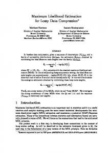
In our simulation study we consider …ve di¤erent estimation procedures, speci…cally the GLS estimator with positive de…nite corrected variance covariance matrix, the Bayes estimator based on the iterative mode estimation suggested in Lindley and Smith (1972), which we will refer to as "Bayes", the Gibbs sampler approach to Bayesian estimation suggested in Pesaran et al. (1999), which will be referred to as "Gibbs", as well as Nelder-Mead and SA based Maximum Likelihood. To evaluate and compare the results of each estimation approach, we report the Root Mean Square Error (RMSE) of every parameter estimated, as well as their Bias, and, further, the size and power for a standard hypothesis test of (individual) slope coe¢ cients being equal to zero. In the literature to date, typically only diagnostics for the slope coe¢ cients have been reported. Here, we report on diagnostics for the complete set of estimated parameters in the case of K = 3. In order to facilitate the assessment of the relative performance of the …ve estimators considered, we use a graphical presentation for a subset of parameter estimates, while the complete set of our results is presented in tables for the interested reader.18 The Figures presenting RMSEs and Biases of a particular parameter estimate are in general organized as follows: Each …gure has 3 panels, each corresponding to a particular size of the time dimension, i.e., the left panel depicts the case with T = 10, the middle one corresponds to T = 20, the right panel to T = 30. Along the horizontal axis the parameter estimates we depict the paramter estimate with a superscript indicating the size of the cross-sectional dimension, N . Figure 1 shows the RMSE of the estimates for . As we see this …gure shows little di¤erence in performance of GLS, Bayes, Gibbs, and SA, while NM is performing signi…cantly worse. Figure 2. shows the Bias of the for which we observe the same comparative situation as for Figure 1. Figure 3 depicts the RMSE for the select elements of , namely for its …rst row. And as we see NM performs much worse than GLS, Bayes, Gibbs, and SA. Relatively big values of RMSE of NM with respect to other do not allow observing how do the other algorithmd compare to each other. To this end Figure 4. depicts the RMSE of select elements of without reporting on NM. As we see in Figure 4 among GLS, Bayes, Gibbs, and SA, Gibbs is performing signi…cantly worst, and GLS and SA outperform Bayes, with GLS performing best. Figures 5 and 6 report on the bias of the select elements of in the same fasion as 16

For the two variable case, K = 2, we drop the last element of and also the coressponding column and row of . 17 The R2 of each regression is controlled for, with a 95% con…dence band from 0:21 to 0:40. 18 We chose not to include the Nelder-Mead based ML estimates in the graphs as the performance of this estimator is far worse than the others’, thus requiring a di¤erent scale.

13

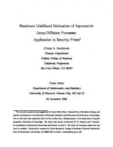
the previous 2 …gures which were reporting on thr RMSE. What we observe in Figure 5 is that NM performs much worse than GLS, Bayes, Gibbs, and SA. Figure 6, which depicts the Bias of the select elements of without reporting on NM, shows that among GLS, Bayes, Gibbs, and SA, Bayes and Gibbs are signi…cantly outperformed by GLS and SA. RMSE of slect elements of , namely its second, ……th, and ninth elements, are shown in Figure 7, which again shows that NM performs much worse than GLS, Bayes, Gibbs, and SA. Figure 8, shows the same results as shown in Figure 7, except that it excludes NM. Figure 8, shows that the performance of SA improves with time dimension, GLS typically performing best among GLS, Bayes, Gibbs, and SA. Figure 9 and 10 show the bias of the select elements of is the same fasion as shown in Figures 7 and 8. These two …gures show that NM performs much worse than GLS, Bayes, Gibbs, and SA, while among GLS, Bayes, Gibbs, and SA, it is SA and GLS that show a relatively better performance with respect to Bayes and Gibbs. Figure 11 presents the empirical size for the hypothesis test of j = 0, j 2 f0; 1; 2g with nominal size of 5%. As we see from the graph, all approaches but ML-SA are heavily over- or undersized. ML-SA is slightly oversized for T = 10. Finally, Figure 12 presents the power for the hypothesis test of 1 = 0 with a nominal size of 5%. As all approaches but ML-SA are heavily over- or under-sized, no information is e¤ectively contained in their power statistics, while SA power properties are reasonable and improve signi…cantly with the cross-sectional dimension. As a further indication of the success of our algorithm, we …nd that, for the samples generated, the value of the likelihood function evaluated at the parameter estimates obtained by ML-SA is better than the values obtained under the true parameter values, supporting the hope that the SA algorithm indeed converges to the global optimum.19 Overall, we conclude that for our speci…c setup, the SA algorithm is a promising approach to implement maximum likelihood estimation and compares reasonably well relative to the GLS and Bayesian solutions. SA being a stochastically global optimization technique raises this concern that if the convergence was achieved. One way to shed light on this issue is to let the SA search an optimum more than once on a speci…c problem or simulataion setting to see that if the the algorithm converges to the same optima. The results discussed before and reported in Tables for SA were based on a one shot run, however we let the SA to run for 10, 50, 100, and 500 times for each simulation setting for 3 regressors case and for N = T = 10. Figure 13. plots power curves for the hypothesis test of 1 = 0 with a nominal size of 5% for these di¤erent SA replications and compares it with the case where SA is run once. As this …gure shows the power features of the SA algorithm do not sustantillay change indicating that the SA setting used in this paper are fairly robust. 19 Indeed the di¤erence is quite substantial in most of the cases, e.g. for the case depicted in Figure 1, the true likelihood value is -99.6274, while the SA algorithm achieves a value of -82.2112. However, admittedly, such a result is not that much of a surprise, as we only consider 100 observations and the number of parameters is relatively large.

14

6

Conclusion

In the current paper we shortly reviewed the di¤erent approaches available for the estimation of random coe¢ cient panel data models with a focus on the Swamy (1970) model. As our main contribution, we then propose a Simulated Annealing algorithm for maximum likelihood estimation, thus o¤ering a concrete implementation of the Maximum Likelihood framework to these class of models. In contrast to standard (local) optimization routines, for which we report problems both in terms of convergence as well as regarding the performance statistics, our SA based implementation of Maximum Likelihood estimatioon seems to be promising for the class of Swamy type models. We employ a simulation study with small to medium time horizon to compare root mean square errors as well as biases of the alternative estimators as well as size and power properties of simple hypothesis tests. Overall, the results suggest that Nelder-Mead based ML estimates generally perform considerably worse than SA based ML and GLS as well as Bayesian approaches, while GLS and SA based ML estimates outperform the Bayesian approaches most of the time. Furthermore, we …nd that SA based ML estimates are the only ones with reasonable size properties for the signi…cance tests. In particular, size and power properties of the signi…cant tests based on ML-SA estimates improve quickly with the magnitude of the cross-sectional dimension. All in all, this paper shows that Maximum Likelihood estimation of simple random coef…cient panel data models is practically feasible once state-of the art optimization algorithms are considered, hence, o¤ering an alternative to the Bayesian approaches prevailing in the literature. Further, SA based maximum likelihood estimates perform strongly for cross-sectional dimensions typically available in macroeconomic panels. Based on these promising results, an extension of SA based Maximum Likelihood estimation to dynamic models and models featuring both random and systematic slope coe¢ cient variation, where a closed form GLS solution is no longer available would be appealing.

7

References 1. Bertsimas, D. and J. Tsitsiklis (1993). Simulated annealing. Statistical Science 8, 10-15. 2. Brooks, S. P. and B. J. T. Morgan (1995). Optimization using simulated annealing. The Statistician 44, 241-257. 3. Chib, S. (2008). Panel data modeling and inference: a bayesian primer. In chapter 15: the econometrics of panel data fundamentals and recent developments in theory and practice, László Mátyás and Patrick Sevestre (eds.). 4. Coleman, T. F. and Y. Li (1994). On the convergence of reáective newton methods for large-scale nonlinear minimization subject to bounds. Mathematical Programming 67, 189-224.

15

5. Coleman, T. F. and Y. Li (1996). An interior, trust region approach for nonlinear minimization subject to bounds. SIAM Journal on Optimization 6, 418-445. 6. Go¤e, W. L., G.D. Ferrier and J. Rogers (1994). Global optimization of statistical functions with simulated annealing. Journal of Econometrics 60, 65-99. 7. Hajek, B. (1988). Cooling schedules for optimal annealing. Mathematical Operations Research 13, 311-329. 8. Hsiao, C., M. H. Pesaran and A. K. Tahmiscioglu (1999). Bayes estimation of short-run coe¢ cients in dynamic panel data models. In C. Hsiao, L.F. Lee, K. Lahiri and M.H. Pesaran (eds.), Analysis of Panels and Limited Dependent Variables Models. Cambridge University press, 268-296. 9. Hsiao, C. (2003). Analysis of panel data. Economic society monographs No.34, 2nd edition. Cambridge University Press. 10. Hsiao, C. and M. H. Pesaran (2004). Random coe¢ cient panel data models. Center for Economic Studies and Ifo Institute for Economic Research CESifo, Working Paper No. 1233. 11. Kirkpatrick, S., C. D. Gerlatt Jr. and M. P. Vecchi (1983). Optimization by simulated annealing. Science 220, 671-680. 12. Lagarius, C. L., J. A. Reeds, M. H. Wright and P. E. Wright (1998). Convergence properties of the Nelder-Mead simplex method in low dimensions. SIAM Journal of Optimization 9, 112-147. 13. Lindley, D. V. and A. F. M. Smith (1972). Bayes estimates for the linear model. Journal of Royal Statistical Society, Series B (Methodological) 34, 1-41. 14. McKinnon, K. I. M. (1998), Convergence of the Nelder-Mead simplex method to a nonstationary point. SIAM Journal of Optimisation 9, 148-158. 15. Metropolis, N., A. W. Rosenbluth, M. N. Rosenbluth, A. H. Teller and E. Teller (1958). Equations of state calculations by fast computing machines. Journal of Chemical Physics 21, 1087-1092. 16. Nelder, J. A. and R. Mead (1965). A simplex method for function minimization. The Computer Journal 7, 308-313. 17. Pincus, M. (1970). A monte carlo method for the approximate solution of certain types of constrained optimization problems. Operations Research 18, 1225-1228. 18. Price, C. J., I. D. Coope and D. Byatt (2002). A convergent variant of the Nelder-Mead algorithm. Journal of Optimization Theory and Application 113, 5-19.

16

19. Romeo, F. and A. Sangiovanni-Vincentelli (1991). A theoretical framework for simulated annealing. Algorithmica 6, 302-345. 20. Swamy, P. A. V. B. (1970). E¢ cient inference in a random coe¢ cient regression model. Econometrica 38, 340-361. 21. van Laarhoven, P. J. and E. H. Aarts (1992). Simulated annealing: theory and applications. Kluwer Academic Publishers Group. 22. Winker, P. and M. Gilli (2004). Editorial: applications of optimization heuristics to estimation and modelling problems. Computational Statistics and Data Analysis 47, 211223.

17

18

8

0

0.5

1

1.5

2

2.5

3

3.5

4

4.5

T = 10

G LS

T = 20

Bayes

G ibbs

SA

NM T = 30

Figure 1. For K = 3, i.e. 3 parameters case, the RMSE for is depicted here. The …gure is divided into 3 panes: the left-most pane correponds to T = 10, the pane in the middle corresponds to T = 20, and the right-most pane =n corresponds to T = 30. The elements on the horizontal axis are shown as N where n is the cross-section size and j takes values of 10, 20, and 30 while j takes a value of 0 for the intercept, a value of 1 for the …rst slope and a value of 2 for the second slope parameter. The vertical axis represents the values of RMSE for di¤erenet estimation approches. The format of this …gure is used for other …gures. The legend of this …gure includes GLS for General Least Square method, Bayes for Bayes approach, Gibbs for Gibbs Sampler, SA for Simulated Annealing based Maximum Likelihood estimates and …nally NM for Nelder-Mead based Maximum Likelihood estimates.

Figures

19

-1

-0.5

0

0.5

1

Figure 2. Bias of

T=10

T=20

Bayes

Gibbs

SA

NM

T=30

for the case of K = 3. See Figure 1. for more details.

GLS

20

Figure 3. RMSE of

0

5

10

15

20

25

T=20

Bayes

Gibbs

SA

NM

T=30

for the case of K = 3, which is reported only for the elements of …rst row of Figure 1.

T=10

GLS

. For more details see

21

T=20

Bayes

Gibbs

SA

T=30

Figure 4. RMSE of exactly as depicted in Figure 3, except that Nelder-Mead is not reported here so as to be able to observe how do the other approaches compare to each other. For more detals see Figure 1.

0

0.2

0.4

0.6

0.8

1

T=10

GLS

22

Figure 5. Bias of

0

1

2

3

4

5

6

7

8

9 T=20

Bayes

Gibbs

SA

NM

T=30

which is reported for the case K = 3, and only for the …rst rowo of

T=10

GLS

. For more details see Figure 1.

23

Figure 6. Bias for

-0.2

0

0.2

0.4

0.6

0.8

1

T=20

Bayes

Gibbs

SA

T=30

which is reported for its …rst row only in the same fashion as Figure 5, while NM is not reported so as to be able to observe the di¤erence between other estimation approaches.

T=10

GLS

24

T=10

GLS

T=20

Bayes

Gibbs

SA

NM

T=30

Figure 7. RMSE for select elements of for the case of K = 3, i.e. for the …rst, …fth and the ninth element. These elements are chose to be among the …rst 10 elements so as to be in common between simulations with di¤erent cross-sectional lengths. For more details see Figure 1.

0

20

40

60

80

100

120

140

160

180

200

25

T=20

Bayes

Gibbs

SA

T=30

Figure 8. RMSE for select elements of …r the case of K = 3 which are depicted here in the same fasion as that of Figure 7 except that NM is not reported so as to be able to observe the di¤erence between other estimation approaches.

0

0.2

0.4

0.6

0.8

1

1.2

T=10

GLS

26

T=10

Figure 9. Bias of select elements of

0

2

4

6

8

10

12

14

16 T=20

Bayes

Gibbs

SA

NM

T=30

for the case of K = 3. For more details see Figure 1 and Figure 7.

GLS

27

T=20

Bayes

Gibbs

SA

T=30

Figure 10. Bias of the select elements of reported in the same fasion as that of Figure 9, except that NM is not reported so as to be able to observe the di¤erence between other estimation approaches. For more details see Figure 1 and 7.

-0.4

-0.2

0

0.2

0.4

0.6

T=10

GLS

28

T=20

Bayes

Gibbs

SA

NM

T=30

=n Figure 11. Empirical size for a hypothesis test of N = 0 with a nominal size of 5%. For more details see Figure 1. NM is not j reported for the case of (N=30 and T=30), which is due to extremely time consuming calculations involved.

0

0.1

0.2

0.3

0.4

0.5

0.6

T=10

GLS

29 0

N=30 and T = 10

0.5 GLS

0 -0.5

0.2

0.4

0.6

0.8

1

Bayes

0

0

Gibbs

N=20 and T = 20

0

N=10 and T = 20

SA

0.5

0.5

0.5

NM

0 -0.5

0.5

1

0 -0.5

0.5

1

0 -0.5

0.5

1

0

N=30 and T = 30

0

N=20 and T = 30

0

N=10 and T = 30

0.5

0.5

0.5

Figure 12. Power for nominal size of 5 % calculated for the hypothesis of 1 = 0 for K = 3. The horizontal axis in each pane of this …gure represents the statistical error considered for the test to be detected. NM is not reported for the case of (N=30 and T=30), which is due to extremely time consuming calculations involved.

0 -0.5

0.5

1

0 -0.5

0 -0.5 0.5

0.5

0 -0.5

0.5

0

0.5

0.5

1

1

N=20 and T = 10

0

N=10 and T = 10

1

0 -0.5

0.2

0.4

0.6

0.8

0.5

0.45

0.4

0.35

0.3

0.25

0.2

0.15

0.1 -0.5

-0.4

-0.3

-0.2 SA1

-0.1 SA10

0 SA50

0.1 SA100

0.2 SA500

0.3

0.4

0.5

Figure 13. Power curves for the hypothesis test of 1 = 0 with a nominal size of 5% for 1, 10, 50, 100, and 500 repetitions of SA for each simulation setting.

30

31

Tables

NM

GLS

Gibbs

k=2

Bayes

SA

NM

GLS

Bayes

Gibbs

SA

NM

0:0696 0:2062 0:1706 extreme

0:0677 0:0679 0:8606 0:0481 0:0433 0:0430 0:0366 0:9157 0:0403 0:0367 0:0370 0:0311 0:1981 0:1837 1:6808 0:1839 0:1712 0:1706 0:1583 1:3409 0:1749 0:1621 0:1628 0:1722 0:1592 0:1432 0:8346 0:1209 0:1163 0:1147 0:1055 1:3331 0:1093 0:1041 0:1038 0:0994 computation time required.

2:2101 1:4811 2:0800

N = 20 0:0887 0:0847 0:0801 0:0798 0:3076 0:0602 0:0561 0:0556 0:0536 1:5034 0:0503 0:0465 0:0467 0:0448 0:2902 0:2484 0:2396 0:2445 0:6808 0:2299 0:2124 0:2111 0:2357 1:1956 0:2166 0:2066 0:2067 0:2186 0:2254 0:2073 0:1966 0:2013 0:6844 0:1530 0:1444 0:1416 0:1557 2:1583 0:1354 0:1280 0:1283 0:1452

N = 30 0:0814 0:2288 0:1769 * Not reported due to

1:0326 2:9744 4:4349

N = 10 0:1233 0:1151 0:1105 0:1156 0:7597 0:0790 0:0757 0:0743 0:0762 0:1284 0:0709 0:0671 0:0670 0:0684 0:3907 0:3663 0:3510 0:3575 1:6951 0:3220 0:2982 0:2971 0:3155 1:8238 0:2956 0:2703 0:2707 0:2913 0:2796 0:2774 0:2577 0:2590 1:1062 0:2002 0:1910 0:1881 0:2114 1:8735 0:1690 0:1610 0:1596 0:1799

k=3

N = 30 0:0775 0:0657 0:0660 0:0684 0:0743 0:0775 0:0432 0:0431 0:0406 0:2568 0:0408 0:0371 0:0374 0:0349 0:1905(1) 0:2324 0:2020 0:1976 0:1880 0:2567 0:2324 0:1737 0:1747 0:1746 0:5227 0:1684 0:1553 0:1572 0:1627 0:4322(1)

3:3305 2:2360

SA

T = 30

N = 20 0:0879 0:0787 0:0771 0:0814 0:7771 0:0604 0:0545 0:0550 0:0555 2:3579 0:0503 0:0463 0:0467 0:0474 0:2905 0:2523 0:2491 0:2507 1:3246 0:2253 0:2124 0:2111 0:2183 1:6837 0:2122 0:2014 0:2029 0:2072

Gibbs

T = 20

1:8046 4:7958

Bayes

T = 10

N = 10 0:1203 0:1088 0:1076 0:1107 1:4179 0:0767 0:0740 0:0731 0:0746 0:1261 0:0667 0:0640 0:0639 0:0637 0:3924 0:3464 0:3414 0:3502 1:7863 0:3079 0:2841 0:2851 0:2949 2:1245 0:2962 0:2833 0:2832 0:2902

GLS

Table 1. RMSE of

9

32

0:1769 0:1850 1:6137

0:1607 0:1416 1:3957

N = 20 0:0096 0:0266 0:6365

N = 30 0:0099 0:0266 0:6385 k=3

0:7965 0:3447 5:8008

0:8507 0:4457 6:3279

0:9673 0:7161 7:4599

k=2

Gibbs

0:0222 0:0565 0:3656

0:0318 0:0779 0:4319

0:0582 0:1082 0:4630

SA

0:0803 0:0268

0:8986

12:5620 0:0374 13:8637

29:4639 0:1497 28:2102

NM

3:0520 0:0287 0:0182 9:4587 0:0567 0:0580

N = 20 0:0096 0:2026 0:9427 0:0316 0:0266 0:6363 0:1997 1:6979 0:4878 6:8147 0:0751 0:6008 0:0100 0:0638 0:1577 0:1570 0:4722 1:0853 0:3969 1:1495 4:8168 0:0619 0:2255 0:4471

N = 30 0:0098 0:1798 0:8690 0:0235 0:0266 0:6384 0:1562 1:4850 0:3764 6:2284 0:0578 0:3745 0:0100 0:0639 0:1590 0:1193 0:3558 1:0028 0:3020 0:8547 4:4978 0:0360 0:1787 0:2032

33:6522 0:0961

9:0495 0:0698

7:4393

8:7655

N = 10 0:0083 0:2669 1:1598 0:0467 19:1716 0:0265 0:6246 0:3297 2:3080 0:8861 8:9569 0:0994 0:5774 0:0585 13:4165 0:0100 0:0632 0:1502 0:2609 0:7809 1:5795 0:6897 2:0493 6:2504 0:0736 0:2699 0:3724 0:0482 0:0761 13:0157

0:2208 0:2845 1:9836

for T = 10 Bayes

N = 10 0:0085 0:0264 0:6256

Table 2. RMSE for elments of GLS

33

0:0878 0:1139 1:1984

0:0779 0:0899 1:0428

N = 20 0:0098 0:0266 0:6376

N = 30 0:0099 0:0266 0:6390 k=3

0:3639 0:2084 3:7168

0:3942 0:2619 4:1059

0:3953 0:4194 4:9689

k=2

Gibbs

0:0119 0:0456 0:3651

0:0362 0:0752 0:5305

0:0209 0:0694 0:4930

SA

34:4747

9:6981 0:0430 0:0368

3:4558 0:0320

18:3358 0:1006 21:6354

6:9149

53:0214 0:1999 33:9283

8:0661 0:0439

NM

N = 30 0:0099 0:0821 0:3789 0:0111 0:0266 0:6390 0:0894 1:0503 0:2103 3:8140 0:0439 0:4302 0:0100 0:0639 0:1595 0:0603 0:2359 0:5016 0:1407 0:5542 2:0801 0:0251 0:1892 0:1579

9:7691 0:0508 0:0431

13:5120 0:0705 48:0377

N = 20 0:0098 0:0953 0:4211 0:0221 23:5169 0:0266 0:6375 0:1274 1:2388 0:3014 4:3538 0:0732 0:5986 0:1094 18:3085 0:0100 0:0638 0:1589 0:0766 0:3227 0:5725 0:1815 0:7596 2:2978 0:0349 0:2063 0:2598 0:0972 0:1040 46:9698

N = 10 0:0093 0:1114 0:4600 0:0379 0:0263 0:6296 0:1896 1:6681 0:4978 5:8284 0:0702 0:6611 0:0099 0:0633 0:1555 0:1185 0:4595 0:7139 0:3112 1:1943 2:7282 0:0550 0:2785 0:3807

0:0966 0:1724 1:5150

for T = 20 Bayes

N = 10 0:0094 0:0263 0:6296

Table 3. RMSE for elments of GLS

34

0:0616 0:0911 1:0705

0:0533 0:0739 0:9331

N = 20 0:0099 0:0266 0:6378

N = 30 0:0099 0:0266 0:6391 k=3

0:2419 0:1709 3:1415

0:2656 0:2122 3:4895

0:3184 0:3554 4:5491

k=2

Gibbs

0:0099 0:0334 0:3693

0:0148 0:0466 0:5012

0:0165 0:0583 0:5058

SA

N = 30 0:0099 0:0558 0:0266 0:6391 0:0766 0:9763 0:0100 0:0639 0:1596 0:0462 0:2060 0:3795 * Not reported due to extreme computation time required. (1) Reported for 500 replications due to extreme computation time reuired.

0:2507 0:0084 0:1810 3:3029 0:0405 0:4414 0:1068 0:4828 1:4927 0:0201 0:1513 0:1596

N = 20 0:0099 0:0662 0:2822 0:0121 0:0266 0:6379 0:1011 1:0769 0:2404 3:6212 0:0550 0:6466 0:0100 0:0638 0:1591 0:0590 0:2440 0:4423 0:1378 0:5713 1:6777 0:0316 0:2537 0:3778

N = 10 0:0095 0:0897 0:3617 0:0238 0:0263 0:6303 0:1719 1:5940 0:4525 5:4065 0:0735 0:6993 0:0099 0:0634 0:1562 0:1023 0:4475 0:6186 0:2626 1:1566 2:2802 0:0586 0:2927 0:3734

0:0804 0:1471 1:4262

for T = 30 Bayes

N = 10 0:0095 0:0263 0:6304

Table 4. RMSE for elments of GLS

25:9210 0:0887 0:1031

49:0963 0:1751

58:6733 0:2688

7:6994(1)

5:1460(1) 0:0355(1) 29:4175 0:1100 0:2763

70:4565

41:4366 0:1540

141:3629 0:7894 279:4861

NM

22:9529

131:8926

35

0:001 0:005

0:006 0:011 0:011

0:001 0:007 0:000

N = 30

N = 10

N = 20

0:001 0:004 0:008

0:004 0:003 0:010

0:001 0:002

0:001 0:005

0:001 0:007

Bayes

0:000 0:001 0:006

0:004 0:001 0:012

0:001 0:002

0:000 0:001

0:001 0:007

Gibbs

T = 10

0:001 0:010 0:001

0:006 0:008 0:019

0:000 0:002

0:002 0:003

0:002 0:004

SA

0:040 0:087 0:099

0:052 0:909 0:200

0:003 0:032

0:042 0:272

0:296 0:697

NM

0:002 0:001 0:001

0:001 0:007 0:014

0:001 0:005

0:001 0:002

0:001 0:001

GLS

0:005 0:001 0:001 0:000 0:158 0:001 0:009 0:004 0:007 0:005 0:405 0:005 0:003 0:001 0:000 0:001 0:612 0:005 * Not reported due to extreme computation time required. (1) Reported for 500 replications due to extreme computation time

0:004 0:007

N = 20

N = 30

0:003 0:001

N = 10

GLS

Table 5. Bias of Gibbs

0:002 0:007

0:000 0:003

0:001 0:003

reuired.

0:000 0:004 0:000

0:000 0:001 0:002

0:001 0:005 0:005

0:000 0:003 0:001

0:001 0:003 0:002

0:001 0:006 0:007

k=3

0:002 0:007

0:000 0:003

0:001 0:003

k=2

Bayes

T = 20

0:001 0:003 0:006

0:000 0:002 0:002

0:001 0:005 0:008

0:001 0:007

0:001 0:002

0:000 0:000

SA

0:190 0:001 0:258

0:372 0:860 0:477

0:121 0:717 0:737

0:072 0:168

0:878 1:275

0:117 0:686

NM

0:000 0:005 0:003

0:003 0:007 0:001

0:002 0:016 0:004

0:001 0:010

0:000 0:013

0:001 0:013

GLS

0:001 0:002 0:003

0:001 0:008 0:001

0:001 0:013 0:005

0:000 0:003

0:001 0:013

0:000 0:009

Bayes

0:001 0:002 0:002

0:001 0:007 0:001

0:002 0:013 0:005

0:000 0:004

0:001 0:013

0:000 0:008

Gibbs

T = 30

0:000 0:001 0:003

0:001 0:009 0:000

0:002 0:011 0:006

0:001 0:003

0:001 0:000

0:001 0:009

SA

0:385 0:828 0:272

0:209 0:235 0:527

0:018(1) 0:095(1)

0:771 1:344

0:363 0:460

NM

36

0:010 0:027 0:010

0:008 0:026 0:010

N = 10

N = 30

0:010 0:027

N = 30

0:010 0:027 0:010

0:010 0:027

N = 20

N = 20

0:009 0:026

N = 10

0:638 0:064

0:636 0:064

0:625 0:063

0:639

0:637

0:626

Table 6. Bias of elements of GLS

0:159

0:158

0:150

0:169 0:017 0:011

0:184 0:025 0:018

0:228 0:025 0:007

0:150 0:027

0:161 0:023

0:188 0:038

for T = 10

1:352 0:066

1:473 0:079

1:842 0:120

1:254

1:389

1:592

Bayes

0:918

0:961

1:259

0:855 0:079 0:039

0:920 0:094 0:060

1:100 0:102 0:026

k=3

0:785 0:096

0:831 0:083

0:921 0:125

k=2

6:049 0:240

6:504 0:270

8:141 0:398

5:622

6:041

6:855

Gibbs

4:388

4:644

5:721

0:008 0:007 0:004

0:014 0:012 0:002

0:024 0:014 0:005

0:007 0:005

0:012 0:007

0:019 0:011

0:018 0:009

0:001 0:008

0:021 0:013

0:049

0:012

0:098

SA

0:036

0:084

0:090

1:279 0:018 0:018

0:478 0:027 0:011

4:139 0:021 0:011

0:022 0:027

2:124 0:023

9:905 0:001

3:792 0:036

2:860 0:063

5:608 0:056

0:183

4:231

6:722

NM

2:012

2:616

4:057

37

0:010 0:027 0:010

0:009 0:026 0:010

N = 10

N = 30

0:010 0:027

N = 30

0:010 0:027 0:010

0:010 0:027

N = 20

N = 20

0:009 0:026

N = 10

0:639 0:064

0:638 0:064

0:630 0:063

0:639

0:638

0:630

Table 7. Bias of elements of GLS

0:160

0:159

0:156

0:076 0:028 0:009

0:086 0:034 0:010

0:093 0:049 0:009

0:072 0:027

0:079 0:032

0:079 0:037

for T = 20

0:943 0:072

1:069 0:085

1:320 0:089

0:931

1:015

1:199

Bayes

0:454

0:501

0:581

0:372 0:094 0:033

0:410 0:113 0:036

0:432 0:171 0:044

k=3

0:358 0:091

0:384 0:099

0:372 0:124

k=2

3:668 0:236

4:107 0:270

5:183 0:336

3:571

3:849

4:444

Gibbs

2:023

2:206

2:507

0:001 0:003 0:002

0:005 0:002 0:003

0:009 0:002 0:006

0:000 0:003

0:004 0:001

0:004 0:006

0:061 0:014

0:095 0:015

0:071 0:017

0:027

0:041

0:027

SA

0:024

0:044

0:071

2:361 0:020 0:017

5:265 0:014 0:021

3:175 0:026 0:007

1:007 0:023

12:925 0:012

2:990 0:032

3:980 0:042

4:352 0:039

7:583 0:076

1:941

9:157

9:838

NM

5:730

9:282

7:722

38

0:010 0:027

0:009 0:026 0:010

N = 30

N = 10

0:638 0:064

0:630 0:063

0:639

0:638

0:630

0:159

0:156 0:059 0:030 0:013

0:074 0:043 0:016

0:049 0:026

0:055 0:031

0:066 0:039

for T = 30

0:920 0:067

1:271 0:063

0:833

0:914

1:124

Bayes

0:388

0:504 0:273 0:102 0:040

0:338 0:154 0:057

k=3

0:237 0:086

0:258 0:099

0:300 0:127

k=2

3:390 0:226

4:801 0:259

3:007

3:268

4:045

Gibbs

0:010 0:052 0:246 0:027 0:639 0:030 0:877 0:096 3:165 0:010 0:064 0:160 0:012 0:085 0:343 0:039 0:257 * Not reported due to extreme computation time required. (1) Reported for 500 replications due to extreme computation time reuired.

N = 30

0:010 0:027 0:010

0:010 0:027

N = 20

N = 20

0:009 0:026

N = 10

Table 8. Bias of elements of GLS

1:449

1:606

2:088

0:000 0:003 0:001

0:001 0:003 0:001

0:005 0:005 0:001

0:001 0:002

0:001 0:001

0:002 0:003

0:099 0:013

0:141 0:004

0:102 0:003

0:039

0:066

0:017

SA

0:023

0:073

0:064

8:857 0:014 0:022

9:764 0:048

16:202 0:066

3:094(1)

0:888(1) 0:023(1) 6:569 0:022 0:036

15:163

40:943

13:652 0:007

38:296 0:016

NM

8:373

24:607

39

0:4629 0:5803 0:5584 0:4714 0:3559 0:3266 0:5069 0:6361 0:3888 0:6715

0:4934 0:6182 0:5831 0:5076 0:3959 0:3428 0:5329 0:6644 0:4060 0:6785

2 1 2 2 2 3 2 4 2 5 2 6 2 7 2 8 2 9 2 10

2 1 2 2 2 3 2 4 2 5 2 6 2 7 2 8 2 9 2 10

GLS

0:7348 0:7255 0:6700 0:7832 0:8240 0:9135 0:7914 0:7305 0:7647 0:7022

0:6649 0:6037 0:6252 0:6593 0:7073 0:7698 0:6530 0:6233 0:6609 0:6259

Bayes

Table 9. RMSE of

0:5977 0:7909 0:7570 0:6162 0:4482 0:3345 0:6624 0:8559 0:4514 0:8877

0:5870 0:7804 0:7624 0:6053 0:4123 0:3258 0:6593 0:8585 0:4508 0:9211

63:7078 27:2849 68:7718 50:4913 46:5562 72:2964 38:3067 1:0598 75:4001 53:3191

NM 0:2720 0:2958 0:3078 0:3794 0:2628 0:2622 0:2643 0:2611 0:3330 0:4039

GLS 0:4802 0:4329 0:4183 0:4192 0:5069 0:4892 0:4594 0:5248 0:4307 0:4258

Bayes

k=3

0:2616 0:3210 0:3370 0:4438 0:2409 0:2381 0:2568 0:2356 0:3771 0:4758

k=2

Gibbs

T = 20

0:2739 0:3196 0:3043 0:3799 0:2662 0:2654 0:2800 0:2640 0:3311 0:4010

SA

0:4992 71:2622 0:2795 0:5165 0:0001 0:2892 0:6088 17:3471 0:3014 0:4653 0:3239 0:3034 0:6305 56:5067 0:3132 0:4454 0:3392 0:3088 0:5044 14:1583 0:3933 0:4454 0:4470 0:3905 0:4098 74:9776 0:2691 0:5224 0:2466 0:2732 0:3622 137:2633 0:2637 0:5329 0:2388 0:2705 0:5022 18:2778 0:2651 0:5009 0:2564 0:2703 0:6882 0:7929 0:2659 0:5678 0:2419 0:2836 0:4647 99:1627 0:3434 0:4811 0:3814 0:3405 0:6709 29:6411 0:4059 0:4597 0:4697 0:4028

0:4519 0:5819 0:5700 0:4616 0:3710 0:3355 0:4954 0:6730 0:3919 0:6534

SA

for N = 10 T = 10

Gibbs

2 i

31:6934 55:5201 70:6573 42:4340 3:9928 12:8555 39:0051 33:3234 19:8100 67:4719

16:3016 45:1275 63:1585 33:5006 3:8927 8:5457 49:8327 60:0515 11:0525 48:3167

NM

0:2448 0:2467 0:2363 0:2365 0:2426 0:4766 0:2351 0:3816 0:2402 0:3346

0:2443 0:2403 0:2385 0:2334 0:2366 0:4738 0:2352 0:3808 0:2360 0:3255

GLS

0:5011 0:5122 0:5110 0:5302 0:5497 0:4500 0:5283 0:4491 0:5750 0:4621

0:4699 0:4659 0:4602 0:4850 0:5208 0:4323 0:5160 0:4157 0:5158 0:4270

Bayes

0:2445 0:2578 0:2395 0:2360 0:2312 0:5467 0:2240 0:4372 0:2295 0:3737

0:2467 0:2507 0:2441 0:2329 0:2250 0:5504 0:2250 0:4440 0:2266 0:3691

Gibbs

T = 30

2:4188 79:5303 0:2399 0:4408 5:6540 83:9833 14:8171 20:4056 22:5026 17:2429

NM

0:2431 1:8964 0:2486 4:7263 0:2338 24:3974 0:2344 0:4323 0:2434 1:6944 0:4692 9:4557 0:2349 0:3025 0:3709 33:8160 0:2416 0:6135 0:3251 14:9859

0:2444 0:2383 0:2395 0:2341 0:2396 0:4723 0:2386 0:3818 0:2369 0:3228

SA

40

2 1 2 2 2 3 2 4 2 5 2 6 2 7 2 8 2 9 2 10 2 11 2 12 2 13 2 14 2 15 2 16 2 17 2 18 2 19 2 20

0:6207 0:5432 0:5022 0:4921 0:6009 0:4648 0:3405 0:8006 0:4218 0:4897 0:7462 0:6106 0:4371 0:4030 0:4251 0:4366 0:6253 0:6243 0:5430 0:4067

GLS

0:6564 0:6282 0:6804 0:6712 0:6645 0:7014 0:8177 0:6286 0:6883 0:6559 0:6520 0:6429 0:7110 0:7848 0:7028 0:7378 0:6278 0:6609 0:5896 0:7247

Bayes

Table 10. RMSE of

0:8497 0:7321 0:6676 0:6281 0:8257 0:6027 0:3507 1:1060 0:5321 0:6479 1:0171 0:8329 0:5499 0:5006 0:5442 0:5449 0:8590 0:8475 0:7288 0:5007

Gibbs

0:9540 0:8095 0:8140 0:8398 0:8184 0:5401 0:5366 1:0071 0:5346 0:7193 0:8489 0:7518 0:6722 0:5248 0:5553 0:5944 0:8166 0:8033 0:7857 0:5044

SA 0:8791 89:6315 44:2400 183:5017 39:3319 39:0726 103:4461 125:6822 11:6543 52:7200 92:6902 0:7980 102:1711 34:2118 89:6809 44:2103 104:9858 44:4210 32:1057 9:5909

NM

for N = 20 and k = 2 T = 10

2 i

0:2918 0:2902 0:3342 0:3893 0:3355 0:3616 0:3015 0:3027 0:3360 0:2708 0:3355 0:4608 0:4301 0:2870 0:2784 0:3007 0:4497 0:4281 0:2691 0:2979

GLS 0:5209 0:5335 0:4945 0:4915 0:4659 0:4621 0:5153 0:4848 0:4478 0:5386 0:4468 0:4412 0:4301 0:5066 0:4819 0:5237 0:4397 0:4174 0:5420 0:5097

Bayes 0:3050 0:3027 0:3763 0:4626 0:3790 0:4210 0:3364 0:3325 0:3936 0:2775 0:0001 0:5610 0:5161 0:3038 0:2888 0:3215 0:5426 0:5156 0:2666 0:3356

Gibbs

T = 20 0:3523 0:3442 0:3533 0:4227 0:3458 0:4254 0:3751 0:3563 0:4030 0:3500 0:3430 0:5659 0:5392 0:3160 0:4184 0:3713 0:5477 0:4680 0:3071 0:4079

SA 80:3716 26:2779 123:0244 168:6602 6:4161 26:0075 81:6751 109:4561 59:1022 86:8386 60:2645 1:8624 0:7959 50:4135 0:6637 56:5905 254:4994 6:4286 0:8681 9:4375

NM 0:2886 0:2401 0:2729 0:2284 0:2594 0:2403 0:2397 0:4265 0:4028 0:2404 0:2360 0:2429 0:2979 0:2374 0:2351 0:2439 0:3164 0:2451 0:2882 0:2342

GLS 0:4047 0:4260 0:4156 0:4457 0:4136 0:4518 0:4644 0:3943 0:3526 0:4616 0:4410 0:4171 0:3900 0:4300 0:4182 0:4518 0:3691 0:4197 0:3797 0:4866

Bayes 0:3233 0:2556 0:2984 0:2351 0:2878 0:2414 0:2395 0:4955 0:4668 0:2398 0:2465 0:2479 0:3367 0:2436 0:2396 0:2528 0:3619 0:2546 0:3234 0:2238

Gibbs

T = 30 0:3161 0:2873 0:3063 0:2266 0:2820 0:2430 0:2450 0:4475 0:4139 0:2417 0:2646 0:2623 0:3066 0:2423 0:2391 0:2625 0:3294 0:2641 0:3792 0:2389

SA

145:3215 0:6742 0:7063 35:4080 130:8303 3:3264 32:7781 89:3733 136:8385 79:9570 3:9552 45:4664 67:5432 56:9388 17:2376 72:1066 130:1823 111:3249 86:4807 78:5364

NM

41

2 1 2 2 2 3 2 4 2 5 2 6 2 7 2 8 2 9 2 10 2 11 2 12 2 13 2 14 2 15 2 16 2 17 2 18 2 19 2 20

0:7057 0:5975 0:5416 0:5125 0:6314 0:4944 0:3469 0:8284 0:4477 0:5218 0:7616 0:6473 0:4727 0:4284 0:4595 0:4699 0:6590 0:6626 0:6024 0:4443

GLS

0:7353 0:7386 0:7642 0:8039 0:7372 0:8093 0:9097 0:6961 0:7894 0:7538 0:7421 0:7390 0:7881 0:8827 0:7912 0:8524 0:6647 0:7176 0:6731 0:8394

Bayes

Table 11. RMSE of

0:9097 0:7671 0:6883 0:6380 0:8282 0:6196 0:3558 1:0837 0:5441 0:6561 0:9906 0:8345 0:5744 0:5202 0:5565 0:5649 0:8587 0:8520 0:7773 0:5416

Gibbs

0:9604 1:0321 0:7959 0:7729 0:9299 0:6258 0:5316 1:1818 0:7154 0:7119 1:0939 1:0582 0:9583 0:6219 0:5919 0:8449 1:0378 0:9296 0:9046 0:7246

SA 28:6736 13:7828 115:9250 0:6742 69:8728 129:9684 128:3891 62:0385 20:3052 31:2215 16:5915 41:4158 21:9550 149:9867 59:3799 25:6750 56:5714 14:4588 23:7671 142:2349

NM

for N = 20 and k = 3 T = 10

2 i

0:2981 0:2966 0:3436 0:4034 0:3456 0:3554 0:3113 0:3087 0:3542 0:2786 0:3411 0:4605 0:4447 0:2941 0:2881 0:3103 0:4488 0:4455 0:2816 0:3074

GLS 0:5591 0:5789 0:5213 0:4611 0:5182 0:4934 0:5279 0:5376 0:5045 0:6141 0:5192 0:4605 0:4794 0:5478 0:5375 0:5526 0:4447 0:4464 0:5893 0:5682

Bayes 0:3084 0:3087 0:3817 0:4654 0:3830 0:4053 0:3423 0:3358 0:4052 0:2849 0:0001 0:5471 0:5201 0:3071 0:2974 0:3273 0:5325 0:5248 0:2775 0:3400

Gibbs

T = 20 NM

GLS

Bayes

Gibbs

SA

NM

0:3740 167:4520 0:2934 0:4217 0:3257 0:3580 96:8425 0:4221 12:6760 0:2441 0:4369 0:2583 0:2436 0:6163 0:3715 106:7368 0:2756 0:4580 0:2988 0:3027 0:6319 0:4803 310:4135 0:2308 0:4671 0:2355 0:2254 12:2425 0:4493 5:8840 0:2683 0:4467 0:2935 0:2777 87:6797 0:3816 11:5639 0:2495 0:4880 0:2500 0:2573 1:3304 0:4103 52:5696 0:2426 0:4849 0:2429 0:2591 26:8849 0:3563 77:9251 0:4307 0:4148 0:4941 0:4408 84:9064 0:4506 35:7418 0:4104 0:3766 0:4689 0:4359 199:8180 0:3961 55:3462 0:2448 0:4982 0:2446 0:3386 86:4342 0:4182 58:4903 0:2385 0:4672 0:2466 0:2420 1:9834 0:6279 1:6384 0:2470 0:4460 0:2498 0:2910 72:8172 0:4954 0:7940 0:3020 0:4213 0:3385 0:3149 57:5115 0:4019 20:6482 0:2369 0:4492 0:2420 0:2588 27:1786 0:3342 0:6176 0:2436 0:4632 0:2473 0:2348 6:8208 0:3721 23:1361 0:2460 0:4681 0:2534 0:2956 91:0285 0:5724 52:9084 0:3157 0:4244 0:3568 0:3382 363:2792 0:5188 4:6164 0:2456 0:4512 0:2530 0:2371 92:1930 0:4211 1:3881 0:2977 0:4058 0:3306 0:3223 49:8941 0:3309 7:7185 0:2383 0:5258 0:2277 0:2323 83:6513

SA

T = 30

42

GLS 2 0:6489 1 2 0:51 2 2 0:5746 3 2 0:4855 4 2 0:516 5 2 0:4938 6 2 0:487 7 2 0:3812 8 2 0:4712 9 2 0:4401 10 2 0:455 11 2 0:5364 12 2 0:4224 13 2 0:7268 14 2 0:6385 15 2 0:5892 16 2 0:5099 17 2 0:5009 18 2 0:3878 19 2 0:4156 20 2 0:4967 21 2 0:4362 22 2 0:4528 23 2 0:4249 24 2 0:5686 25 2 0:5622 26 2 0:6015 27 2 0:4511 28 2 0:4706 29 2 0:6116 30 (1) Reported

Bayes 0:5914 0:6033 0:6206 0:6425 0:6011 0:6299 0:6403 0:6627 0:6401 0:6497 0:6589 0:6284 0:6579 0:5822 0:5753 0:5961 0:6074 0:5959 0:6544 0:6598 0:6485 0:6347 0:6746 0:6827 0:6165 0:5748 0:5744 0:6181 0:6494 0:5992 for 500

Table 12. RMSE of

for N = 30 and k = 2 T = 10 Gibbs SA NM 0:8974 1:0341 1:8135 0:6788 1:277 13:1683 0:7803 0:9794 44:7891 0:6411 0:9814 70:2349 0:6976 1:231 6:9859 0:6467 1:069 6:1881 0:6365 0:8958 48:9055 0:4673 0:7159 4:9623 0:6092 0:8512 35:7412 0:5666 0:8622 66:5863 0:5834 0:9118 3:4916 0:7045 1:0013 4:0136 0:5317 0:8753 0:5017 0:9812 1:3197 0:9723 0:8792 1:0029 29:449 0:8107 1:043 3:5425 0:6925 0:8252 57:3929 0:6645 0:9183 2:851 0:4739 0:8094 2:3822 0:5119 0:8445 77:9949 0:6523 0:8736 18:626 0:5475 0:8379 11:0895 0:5841 0:939 8:843 0:5306 0:8642 9:3996 0:7714 1:1221 12:982 0:7568 1:1202 27:4141 0:8288 1:0867 2:0987 0:5809 0:814 0:5143 0:6079 1:0091 16:3491 0:8306 1:1101 52:0107 replications due to extreme

2 i

T = 20 GLS Bayes Gibbs SA 0:3008 0:5046 0:32 0:3964 0:384 0:4619 0:4584 0:551 0:2935 0:5287 0:3158 0:5158 0:3096 0:4668 0:3504 0:5264 0:2873 0:526 0:295 0:3685 0:4382 0:4706 0:5273 0:6729 0:4411 0:4571 0:5337 0:7718 0:2698 0:5938 0:2655 0:4988 0:3091 0:5038 0:3485 0:5298 0:3484 0:4826 0:4103 0:6119 0:2667 0:6074 0:0001 0:3246 0:274 0:5102 0:2817 0:4897 0:4177 0:4796 0:5064 0:7414 0:5282 0:4403 0:6438 0:8022 0:2738 0:5691 0:2658 0:4122 0:3108 0:4728 0:3521 0:4891 0:5249 0:4597 0:6365 0:6784 0:2807 0:5026 0:2829 0:4646 0:2991 0:494 0:3296 0:4876 0:3634 0:4919 0:4223 0:8425 0:3103 0:5129 0:3404 0:4868 0:2643 0:5673 0:2502 0:3467 0:2812 0:4861 0:2987 0:4278 0:267 0:5681 0:2604 0:359 0:3304 0:4664 0:376 0:5332 0:3096 0:4615 0:3501 0:5733 0:4633 0:4512 0:5615 0:7601 0:3351 0:4528 0:3846 0:6158 0:297 0:4999 0:3254 0:6817 0:3656 0:4395 0:432 0:5493 computation time reuired. NM 1:6848 0:4211 67:8963 6:0491 4:0561 26:7741 2:8114 3:8796 0:3615 30:1444 12:3369 6:7659 8:7896 3:3657 4:865 1:9641 12:0906 19:9436 9:2357 17:6101 3:5374 6:1601 18:083 26:0841 10:9665 19:6656 19:6368 0:3417 20:0123 0:3268

GLS 0:2413 0:2624 0:2281 0:2495 0:294 0:3184 0:2391 0:2512 0:4269 0:248 0:2281 0:2564 0:2363 0:2446 0:35 0:2695 0:298 0:3984 0:2251 0:2438 0:2425 0:2694 0:3032 0:2371 0:235 0:2884 0:2465 0:3288 0:2361 0:2318

Bayes 0:4669 0:4219 0:4965 0:3973 0:4036 0:377 0:4771 0:4365 0:3935 0:4275 0:4949 0:4277 0:4347 0:4224 0:3827 0:4062 0:4142 0:367 0:4405 0:4307 0:4028 0:4011 0:404 0:4382 0:4619 0:3887 0:4156 0:3989 0:4644 0:4785

T = 30 Gibbs 0:2486 0:2788 0:2134 0:2659 0:3322 0:3604 0:2223 0:2576 0:4986 0:2587 0:214 0:2697 0:2416 0:2513 0:4026 0:2997 0:3325 0:4645 0:2204 0:2591 0:2517 0:2922 0:3422 0:2338 0:2217 0:3236 0:26 0:3776 0:2304 0:2204 SA 0:3049 0:3217 0:248 0:3524 0:3651 0:3946 0:3206 0:3629 0:5301 0:3319 0:2316 0:3005 0:2986 0:3428 0:4502 0:3372 0:4367 0:5153 0:2862 0:3296 0:2844 0:2743 0:3576 0:343 0:2924 0:312 0:3286 0:4077 0:3046 0:2652

NM1 0:277 37:271 11:226 35:769 15:984 7:575 28:844 16:401 2:438 8:779 24:784 0:265 13:400 8:911 21:263 8:903 27:898 11:654 5:602 1:852 3:408 13:236 2:830 8:640 2:028 15:400 4:976 17:467 21:734 20:085

43

2 i

2 1 2 2 2 3 2 4 2 5 2 6 2 7 2 8 2 9 2 10 2 11 2 12 2 13 2 14 2 15 2 16 2 17 2 18 2 19 2 20 2 21 2 22 2 23 2 24 2 25 2 26 2 27 2 28 2 29 2 30

GLS Bayes 0:6903 0:6769 0:5611 0:6811 0:6128 0:7024 0:5264 0:7216 0:5466 0:6973 0:5293 0:7135 0:5241 0:6964 0:4099 0:8046 0:4928 0:7271 0:4693 0:7456 0:4771 0:7974 0:5621 0:7478 0:4688 0:7631 0:7531 0:6598 0:668 0:6337 0:6211 0:6856 0:5402 0:6557 0:5323 0:6956 0:4241 0:7845 0:4428 0:7546 0:5332 0:7306 0:4611 0:7214 0:4852 0:7693 0:4553 0:798 0:6353 0:6959 0:6154 0:6899 0:6568 0:6601 0:4861 0:702 0:5009 0:7526 0:648 0:68 * Not reported due to

Table 13. RMSE of

for N = 30 and k = 3 T = 10 Gibbs SA NM 0:9014 1:0693 46:8354 0:7161 0:9966 1:407 0:7937 1:1679 0:7148 0:6648 1:124 43:4173 0:703 1:0434 0:7328 0:6745 0:8973 70:5977 0:6575 0:8844 216:9729 0:4781 0:8902 2:8535 0:6138 0:976 0:997 0:5779 1:0223 105:9677 0:5886 0:9056 158:1694 0:7154 0:9927 0:7218 0:5743 0:7308 0:6366 0:9709 1:2543 19:4134 0:8794 1:2871 108:0284 0:8213 1:1464 1:5759 0:7032 1:0554 57:7077 0:6658 0:9306 128:5461 0:5061 0:8402 102:9454 0:5301 1:0398 383:0956 0:6694 1:0051 3:5156 0:5583 1:0058 114:2256 0:6001 1:0328 65:9942 0:5456 0:8432 43:2115 0:8106 1:2079 30:878 0:7897 1:3102 87:5886 0:8437 1:127 98:8852 0:6061 0:9065 133:6995 0:6246 1:0426 96:0258 0:841 1:0616 78:1395 extreme computation time GLS 0:3091 0:3888 0:2988 0:3215 0:2933 0:4504 0:455 0:2772 0:3209 0:3616 0:2721 0:2788 0:4305 0:5415 0:2777 0:316 0:5474 0:2882 0:3054 0:369 0:3157 0:2715 0:2885 0:2756 0:3404 0:3212 0:4681 0:3338 0:3052 0:3824 required.

Bayes 0:5253 0:4894 0:5686 0:5364 0:5689 0:4985 0:4952 0:6437 0:542 0:5032 0:6485 0:5541 0:5059 0:4651 0:5957 0:529 0:4941 0:5331 0:5165 0:5128 0:5425 0:6114 0:5403 0:5834 0:5186 0:5043 0:4643 0:4859 0:5574 0:4721

T = 20 Gibbs 0:3277 0:4545 0:3173 0:3581 0:2967 0:5302 0:5376 0:2732 0:3553 0:4178 0:0001 0:2837 0:5057 0:6415 0:2706 0:3536 0:6446 0:2894 0:3311 0:4192 0:3424 0:2574 0:306 0:2683 0:3792 0:3607 0:5558 0:3759 0:3293 0:4389 SA 0:626 0:6399 0:4027 0:5998 0:4535 0:9028 0:5812 0:3966 0:5382 0:6915 0:3352 0:4901 0:7345 0:9803 0:3847 0:7378 0:6608 0:5868 0:5263 0:4715 0:5154 0:3132 0:5156 0:5647 0:654 0:5966 0:6463 0:4569 0:4772 0:5426

NM 0:6183 162:1517 8:0963 0:8654 180:9073 28:6689 62:1570 18:9816 1:2699 4:6716 7:6420 14:9086 5:3736 2:0464 22:4319 0:8203 53:6782 57:8892 26:7983 51:4068 157:1918 0:5868 54:1567 158:5415 130:7487 58:5597 48:6304 112:3219 111:8148 19:9950

GLS 0:2483 0:263 0:2293 0:2536 0:3011 0:329 0:2417 0:2546 0:4442 0:2562 0:2324 0:262 0:2399 0:2455 0:3602 0:2703 0:3016 0:4016 0:2303 0:2506 0:2434 0:2751 0:3069 0:2424 0:2373 0:2974 0:2512 0:3318 0:2417 0:2363

Bayes 0:4969 0:4539 0:5272 0:477 0:4032 0:4355 0:5502 0:463 0:3919 0:4605 0:5213 0:4707 0:4817 0:4317 0:4121 0:4199 0:4234 0:3948 0:5009 0:4473 0:4755 0:434 0:4327 0:4938 0:5036 0:4468 0:4502 0:419 0:4831 0:4958

T = 30 Gibbs 0:2547 0:2772 0:2146 0:2682 0:3377 0:3678 0:2249 0:259 0:51 0:267 0:2185 0:2729 0:2433 0:2503 0:4085 0:2975 0:3327 0:4629 0:2257 0:2654 0:2509 0:2965 0:3431 0:2387 0:2247 0:3288 0:2634 0:3769 0:2357 0:2244

SA NM 0:3059 0:3095 0:2632 0:3162 0:4382 0:5228 0:2392 0:2724 0:4323 0:3084 0:2773 0:3418 0:2142 0:2632 0:449 0:3865 0:3671 0:4874 0:203 0:3607 0:2995 0:3183 0:3945 0:2766 0:2696 0:3435 0:2723 0:4002 0:2768 0:2167

44

0:051 0:070 0:068 0:030 0:132 0:197 0:004 0:109 0:132 0:178

0:051 0:084 0:063 0:039 0:127 0:205 0:005 0:113 0:139 0:151

2 1 2 2 2 3 2 4 2 5 2 6 2 7 2 8 2 9 2 10

2 1 2 2 2 3 2 4 2 5 2 6 2 7 2 8 2 9 2 10

GLS

0:340 0:260 0:242 0:364 0:466 0:612 0:344 0:238 0:452 0:170

0:244 0:131 0:140 0:223 0:349 0:461 0:224 0:086 0:333 0:045

Bayes

Table 14. Bias of

2 i

0:170 0:352 0:334 0:187 0:053 0:063 0:234 0:393 0:040 0:446

0:183 0:353 0:357 0:210 0:056 0:050 0:249 0:410 0:055 0:498

Gibbs

SA

0:075 0:051 0:060 0:065 0:159 0:230 0:048 0:088 0:160 0:119

0:065 0:062 0:056 0:050 0:144 0:214 0:022 0:116 0:149 0:153

for N = 10 T = 10

7:608 5:062 4:910 1:664 7:062 13:892 2:222 0:475 16:311 3:929

6:949 7:517 12:095 8:453 5:290 8:901 6:225 0:355 12:544 8:680

NM

0:145 0:056 0:042 0:049 0:183 0:188 0:137 0:194 0:008 0:071

0:145 0:055 0:044 0:051 0:178 0:188 0:135 0:194 0:011 0:073

GLS

0:205 0:119 0:089 0:006 0:296 0:287 0:232 0:348 0:077 0:028

0:146 0:042 0:022 0:065 0:227 0:244 0:162 0:286 0:012 0:088

Bayes

0:000 0:036 0:051 0:158 0:120 0:128 0:063 0:137 0:090 0:185

k=3

0:068 0:041 0:053 0:167 0:113 0:126 0:059 0:135 0:094 0:194

k=2

Gibbs

T = 20

2:379 8:836 11:012 5:792 0:956 1:355 7:595 11:760 2:685 9:671

NM

0:151 6:288 0:063 10:460 0:052 10:156 0:043 7:429 0:189 0:959 0:197 2:296 0:143 3:912 0:196 2:182 0:018 4:217 0:060 10:337

0:148 0:056 0:050 0:044 0:183 0:193 0:136 0:198 0:011 0:064

SA

0:085 0:045 0:068 0:082 0:134 0:256 0:124 0:163 0:128 0:078

0:081 0:047 0:064 0:084 0:132 0:258 0:125 0:167 0:121 0:074

GLS

0:245 0:231 0:258 0:280 0:339 0:022 0:324 0:051 0:338 0:103

0:194 0:176 0:185 0:221 0:285 0:089 0:282 0:007 0:275 0:046

Bayes

0:029 0:016 0:010 0:027 0:086 0:346 0:075 0:244 0:079 0:151

0:022 0:016 0:004 0:026 0:082 0:355 0:074 0:256 0:070 0:151

Gibbs

T = 30

0:091 0:052 0:073 0:091 0:134 0:241 0:127 0:148 0:133 0:065

0:087 0:051 0:067 0:089 0:132 0:253 0:129 0:167 0:125 0:069

SA

0:374 0:132 0:702 0:367 0:064 0:870 0:116 2:036 0:101 0:882

0:438 3:947 0:071 0:392 0:322 4:455 1:251 1:709 1:756 1:266

NM

45

2 1 2 2 2 3 2 4 2 5 2 6 2 7 2 8 2 9 2 10 2 11 2 12 2 13 2 14 2 15 2 16 2 17 2 18 2 19 2 20

0:123 0:050 0:018 0:042 0:115 0:029 0:190 0:284 0:079 0:004 0:210 0:106 0:071 0:082 0:064 0:082 0:126 0:116 0:033 0:090

GLS

0:156 0:198 0:264 0:282 0:203 0:338 0:526 0:059 0:324 0:247 0:082 0:200 0:327 0:423 0:336 0:345 0:149 0:195 0:139 0:359

Bayes

Table 15. Bias of

2 i

0:437 0:329 0:282 0:198 0:420 0:211 0:035 0:650 0:148 0:252 0:552 0:408 0:154 0:129 0:167 0:146 0:439 0:421 0:317 0:125

Gibbs

0:232 0:121 0:106 0:026 0:188 0:010 0:143 0:381 0:018 0:075 0:269 0:167 0:021 0:030 0:006 0:019 0:213 0:180 0:131 0:038

SA 0:854 15:680 8:936 29:889 9:831 7:823 15:319 14:964 2:947 11:452 17:311 0:749 13:852 6:272 17:335 9:245 18:517 9:472 6:358 2:429

NM

for N = 20 and k = 2 T = 10 0:093 0:089 0:016 0:078 0:016 0:032 0:033 0:045 0:027 0:098 0:027 0:162 0:105 0:079 0:092 0:073 0:145 0:128 0:124 0:025

GLS 0:288 0:285 0:181 0:127 0:162 0:133 0:230 0:215 0:147 0:292 0:163 0:044 0:023 0:244 0:239 0:257 0:044 0:054 0:319 0:215

Bayes 0:004 0:001 0:089 0:202 0:092 0:147 0:070 0:053 0:142 0:011 0:000 0:303 0:238 0:015 0:003 0:021 0:279 0:258 0:041 0:077

Gibbs

T = 20 0:062 0:060 0:005 0:090 0:004 0:053 0:010 0:023 0:052 0:072 0:019 0:190 0:133 0:064 0:062 0:054 0:175 0:143 0:101 0:003

SA 9:463 3:515 14:939 17:169 1:150 3:636 11:710 11:926 7:976 9:732 7:502 0:060 0:462 7:524 0:629 8:319 25:236 1:192 0:173 10:198

NM 0:034 0:030 0:001 0:059 0:011 0:082 0:086 0:202 0:176 0:088 0:048 0:070 0:055 0:062 0:069 0:053 0:077 0:054 0:040 0:125

GLS 0:101 0:176 0:157 0:233 0:140 0:251 0:255 0:016 0:015 0:237 0:205 0:217 0:094 0:197 0:199 0:213 0:035 0:187 0:081 0:301

Bayes 0:108 0:035 0:069 0:001 0:082 0:025 0:029 0:295 0:264 0:030 0:014 0:010 0:129 0:001 0:009 0:010 0:157 0:008 0:113 0:074

Gibbs

T = 30 0:047 0:014 0:015 0:056 0:023 0:075 0:079 0:207 0:173 0:081 0:037 0:059 0:057 0:051 0:061 0:038 0:081 0:046 0:060 0:114

SA

16:180 0:625 0:652 4:399 14:316 0:318 5:450 12:966 14:548 14:039 0:868 6:924 8:913 6:170 2:043 11:473 21:861 18:275 12:612 12:936

NM

46

2 1 2 2 2 3 2 4 2 5 2 6 2 7 2 8 2 9 2 10 2 11 2 12 2 13 2 14 2 15 2 16 2 17 2 18 2 19 2 20

0:140 0:062 0:015 0:031 0:119 0:021 0:187 0:271 0:072 0:003 0:192 0:093 0:066 0:067 0:066 0:083 0:130 0:116 0:064 0:069

GLS

0:275 0:319 0:367 0:425 0:315 0:455 0:623 0:186 0:436 0:361 0:201 0:307 0:430 0:535 0:434 0:483 0:229 0:286 0:261 0:463

Bayes

Table 16. Bias of

2 i

0:440 0:328 0:269 0:202 0:408 0:215 0:029 0:610 0:149 0:241 0:512 0:379 0:152 0:141 0:152 0:140 0:423 0:403 0:341 0:142

Gibbs

0:245 0:204 0:105 0:079 0:233 0:055 0:116 0:416 0:055 0:090 0:333 0:256 0:067 0:021 0:005 0:030 0:293 0:249 0:198 0:025

SA 7:119 4:713 23:399 0:643 15:453 26:731 30:698 14:323 4:667 7:983 5:863 10:067 5:271 30:446 11:328 5:774 11:686 4:842 6:679 27:704

NM

for N = 20 and k = 3 T = 10 0:090 0:087 0:016 0:068 0:015 0:024 0:034 0:045 0:024 0:098 0:031 0:153 0:107 0:082 0:089 0:075 0:143 0:136 0:129 0:027

GLS 0:327 0:346 0:249 0:154 0:226 0:196 0:268 0:288 0:231 0:378 0:246 0:104 0:093 0:301 0:299 0:306 0:097 0:121 0:370 0:300

Bayes 0:004 0:001 0:086 0:184 0:087 0:132 0:066 0:049 0:134 0:013 0:000 0:284 0:232 0:008 0:002 0:015 0:270 0:258 0:050 0:070

Gibbs

T = 20 0:060 0:033 0:009 0:089 0:022 0:037 0:003 0:019 0:063 0:064 0:006 0:196 0:131 0:038 0:062 0:039 0:184 0:152 0:094 0:007

SA 9:349 1:902 7:647 14:424 1:405 1:894 4:295 7:387 4:982 6:674 7:212 0:164 0:295 2:921 0:568 3:060 5:415 1:195 0:029 9:437

NM 0:038 0:028 0:001 0:063 0:012 0:083 0:082 0:199 0:179 0:086 0:050 0:074 0:054 0:061 0:067 0:056 0:075 0:055 0:042 0:126

GLS 0:161 0:214 0:215 0:270 0:205 0:286 0:294 0:021 0:052 0:270 0:257 0:257 0:159 0:243 0:255 0:254 0:109 0:230 0:140 0:345

Bayes 0:109 0:035 0:067 0:005 0:079 0:027 0:027 0:287 0:263 0:030 0:010 0:017 0:126 0:002 0:009 0:005 0:151 0:005 0:113 0:077

Gibbs

T = 30 0:057 0:021 0:009 0:050 0:027 0:063 0:063 0:192 0:178 0:065 0:031 0:053 0:062 0:044 0:056 0:032 0:081 0:040 0:044 0:107

SA

12:358 0:562 0:577 2:687 9:910 0:145 4:087 11:519 15:398 9:391 0:516 8:550 6:864 3:433 1:584 8:591 20:809 8:596 7:173 8:498

NM

47

2 i

for N = 30 and k = 2

T = 10 T = 20 GLS Bayes Gibbs SA NM GLS Bayes Gibbs 2 0:140 0:100 0:464 0:340 0:758 0:077 0:220 0:017 1 2 0:012 0:226 0:279 0:254 2:679 0:078 0:083 0:201 2 2 0:082 0:218 0:369 0:251 7:867 0:067 0:245 0:027 3 2 0:010 0:256 0:249 0:207 8:637 0:019 0:158 0:085 4 2 0:038 0:230 0:308 0:300 1:650 0:108 0:276 0:020 5 2 0:010 0:260 0:242 0:195 1:640 0:133 0:050 0:266 6 2 0:022 0:235 0:232 0:151 7:296 0:144 0:043 0:278 7 2 0:099 0:349 0:114 0:055 1:102 0:132 0:331 0:054 8 2 0:032 0:285 0:211 0:135 6:219 0:022 0:195 0:082 9 2 0:058 0:299 0:178 0:109 9:810 0:038 0:134 0:155 10 2 0:039 0:310 0:198 0:156 0:931 0:192 0:412 0:000 11 2 0:006 0:215 0:268 0:185 1:200 0:099 0:258 0:012 12 2 0:067 0:326 0:158 0:119 0:201 0:119 0:048 0:251 13 2 0:173 0:080 0:503 0:374 0:231 0:231 0:034 0:381 14 2 0:139 0:087 0:460 0:317 5:333 0:143 0:314 0:065 15 2 0:104 0:164 0:408 0:310 1:409 0:015 0:180 0:090 16 2 0:039 0:194 0:311 0:184 7:937 0:213 0:035 0:362 17 2 0:010 0:215 0:271 0:175 1:032 0:118 0:228 0:032 18 2 0:100 0:325 0:111 0:051 0:684 0:044 0:192 0:056 19 2 0:087 0:325 0:128 0:060 8:646 0:031 0:137 0:146 20 2 0:011 0:269 0:247 0:188 3:403 0:048 0:212 0:051 21 2 0:073 0:301 0:154 0:088 1:862 0:157 0:346 0:085 22 2 0:040 0:308 0:202 0:150 1:949 0:073 0:212 0:022 23 2 0:085 0:349 0:131 0:102 1:858 0:134 0:332 0:056 24 2 0:066 0:166 0:357 0:284 2:502 0:009 0:142 0:099 25 2 0:054 0:153 0:339 0:279 4:198 0:018 0:151 0:087 26 2 0:108 0:131 0:414 0:301 0:816 0:161 0:009 0:300 27 2 0:045 0:279 0:193 0:113 0:362 0:004 0:126 0:114 28 2 0:033 0:274 0:212 0:160 2:866 0:051 0:201 0:049 29 2 0:102 0:166 0:405 0:338 9:191 0:049 0:093 0:168 30 (1) Reported for 500 replications due to extreme computation time reuired.

Table 17. Bias of SA 0:013 0:144 0:014 0:063 0:043 0:208 0:223 0:036 0:055 0:132 0:129 0:013 0:216 0:328 0:054 0:061 0:274 0:029 0:026 0:138 0:024 0:097 0:003 0:070 0:065 0:065 0:256 0:085 0:032 0:116

NM 0:511 0:914 21:771 2:591 2:657 9:166 2:067 1:680 0:212 15:371 5:789 4:033 4:883 2:552 2:713 1:487 5:645 9:518 4:553 10:691 1:948 2:181 9:059 12:560 4:767 12:439 10:290 0:242 8:427 0:286

GLS 0:061 0:032 0:136 0:029 0:054 0:067 0:154 0:068 0:216 0:051 0:135 0:044 0:065 0:063 0:114 0:019 0:034 0:186 0:097 0:031 0:055 0:007 0:056 0:098 0:134 0:039 0:037 0:092 0:105 0:126

Bayes 0:211 0:152 0:290 0:153 0:090 0:048 0:296 0:178 0:050 0:178 0:286 0:151 0:197 0:172 0:011 0:104 0:107 0:045 0:234 0:159 0:180 0:127 0:081 0:212 0:257 0:066 0:148 0:025 0:244 0:283

T = 30 Gibbs 0:000 0:034 0:086 0:037 0:128 0:143 0:107 0:007 0:310 0:011 0:085 0:019 0:006 0:003 0:197 0:091 0:108 0:277 0:043 0:034 0:006 0:061 0:131 0:042 0:084 0:113 0:027 0:173 0:051 0:075 SA 0:022 0:008 0:095 0:015 0:069 0:091 0:096 0:017 0:222 0:010 0:098 0:012 0:019 0:023 0:140 0:044 0:073 0:201 0:056 0:006 0:024 0:025 0:080 0:044 0:088 0:063 0:003 0:111 0:069 0:084

NM1 17:624 0:277 0:510 4:563 0:829 9:812 25:095 0:621 0:586 27:547 19:038 0:745 0:712 3:266 17:362 0:124 3:762 10:792 18:872 14:256 0:391 16:251 12:738 5:749 1:632 16:583 29:948 23:096 17:160 12:808

48

2 1 2 2 2 3 2 4 2 5 2 6 2 7 2 8 2 9 2 10 2 11 2 12 2 13 2 14 2 15 2 16 2 17 2 18 2 19 2 20 2 21 2 22 2 23 2 24 2 25 2 26 2 27 2 28 2 29 2 30

GLS Bayes 0:137 0:228 0:025 0:337 0:086 0:324 0:007 0:348 0:035 0:331 0:013 0:366 0:017 0:334 0:110 0:492 0:033 0:374 0:061 0:420 0:054 0:440 0:016 0:369 0:056 0:440 0:170 0:222 0:131 0:189 0:110 0:282 0:031 0:311 0:004 0:325 0:091 0:454 0:092 0:427 0:002 0:351 0:083 0:402 0:050 0:408 0:085 0:452 0:073 0:284 0:064 0:278 0:102 0:251 0:035 0:384 0:033 0:390 0:088 0:290 * Not reported due to

Table 18. Bias of

SA NM 0:356 9:052 0:223 0:150 0:293 0:538 0:249 8:273 0:252 0:758 0:213 11:090 0:181 20:922 0:098 0:436 0:178 0:396 0:196 17:685 0:149 1:861 0:227 0:727 0:084 0:648 0:412 3:947 0:414 17:305 0:343 0:021 0:260 12:432 0:196 15:065 0:097 18:691 0:162 35:583 0:219 0:527 0:147 17:508 0:196 12:346 0:116 8:093 0:319 3:229 0:335 15:385 0:312 20:599 0:156 16:361 0:185 12:508 0:295 12:571 computation time

for N = 30 and k = 3

T = 10 Gibbs 0:443 0:285 0:360 0:242 0:292 0:261 0:228 0:095 0:204 0:169 0:175 0:271 0:166 0:484 0:438 0:403 0:296 0:243 0:119 0:120 0:253 0:140 0:186 0:126 0:349 0:342 0:390 0:202 0:206 0:378 extreme

2 i

GLS Bayes 0:072 0:266 0:068 0:155 0:067 0:315 0:018 0:234 0:112 0:316 0:136 0:104 0:145 0:109 0:128 0:407 0:025 0:257 0:043 0:176 0:194 0:453 0:100 0:302 0:114 0:099 0:224 0:027 0:135 0:370 0:016 0:243 0:215 0:037 0:116 0:274 0:046 0:230 0:023 0:190 0:048 0:271 0:157 0:401 0:068 0:280 0:136 0:366 0:011 0:204 0:012 0:219 0:160 0:060 0:005 0:188 0:055 0:263 0:047 0:164 required.

T = 20 Gibbs 0:020 0:186 0:024 0:082 0:028 0:261 0:272 0:052 0:075 0:155 0:000 0:016 0:237 0:364 0:059 0:085 0:353 0:033 0:049 0:132 0:047 0:086 0:024 0:060 0:092 0:089 0:292 0:099 0:041 0:159 SA 0:024 0:151 0:007 0:063 0:004 0:230 0:183 0:036 0:065 0:150 0:104 0:012 0:211 0:318 0:054 0:085 0:247 0:015 0:039 0:090 0:041 0:077 0:036 0:040 0:083 0:080 0:226 0:062 0:038 0:100

NM 0:533 31:841 1:955 0:155 25:717 5:974 10:926 4:135 0:068 1:294 1:593 2:686 1:718 0:397 4:122 0:814 8:551 10:032 5:100 9:319 26:209 0:320 10:216 27:293 21:587 9:543 7:705 20:637 20:451 4:209

GLS 0:063 0:033 0:136 0:029 0:055 0:068 0:156 0:068 0:225 0:047 0:134 0:045 0:069 0:065 0:114 0:020 0:034 0:187 0:097 0:029 0:054 0:005 0:058 0:100 0:132 0:037 0:038 0:094 0:108 0:127

Bayes 0:251 0:199 0:332 0:229 0:125 0:113 0:363 0:241 0:002 0:237 0:335 0:223 0:250 0:213 0:075 0:147 0:135 0:024 0:301 0:204 0:250 0:181 0:136 0:278 0:313 0:127 0:187 0:069 0:293 0:310

T = 30 Gibbs 0:004 0:031 0:088 0:034 0:127 0:142 0:109 0:010 0:314 0:014 0:085 0:016 0:011 0:007 0:192 0:088 0:104 0:272 0:044 0:034 0:004 0:060 0:130 0:046 0:082 0:107 0:024 0:172 0:055 0:077 SA 0:009 0:005 0:070 0:012 0:083 0:101 0:091 0:027 0:176 0:007 0:074 0:001 0:034 0:019 0:129 0:052 0:059 0:186 0:055 0:023 0:018 0:024 0:072 0:047 0:067 0:065 0:008 0:110 0:046 0:070

NM

49

0:003 0:005 0:009

N = 20 0:178 0:405 0:271

0:000 0:000 0:000

0:000 0:000 0:000

0:080 0:087 0:097

0:091 0:130 0:107

0:105 0:083

0:091 0:120 0:127 0:447 0:140 0:216

0:204 0:142 0:354 0:463 0:208 0:235

0:098 0:197 0:109 0:377

0:204 0:132 0:364 0:406 0:000 0:000

0:000 0:000

0:000 0:000

0:002 0:010 0:009

0:006 0:009 0:006 0:000 0:000 0:000

0:000 0:000 0:000

k=3

0:005 0:011

0:004 0:008

0:005 0:008

k=2

Bayes Gibbs

0:068 0:105 0:091

0:055 0:065

0:062 0:072

0:073 0:089

SA

GLS

0:102 0:133 0:277 0:459 0:271 0:199

0:264 0:135 0:818 0:484

0:426 0:136 0:744 0:481

0:092 0:108 0:309 0:460

NM

0:357 0:131 0:811 0:492 0:812 0:271

0:006 0:011 0:004

N = 10 0:172 0:393 0:224

0:000 0:000

0:085 0:094

0:224 0:136 0:310 0:411

GLS

N = 30 0:224 0:004 0:000 0:097 0:198 0:135 0:003 0:000 0:043 0:390 0:009 0:000 0:071 0:303 0:423 0:007 0:000 0:059 0:257 0:007 0:000 0:075 0:691 0:224 0:007 0:000 0:051 * Not reported due to extreme computation time required. (1) Reported for 500 replications due to extreme computation time reuired.

0:005 0:008

N = 30 0:197 0:377

0:000 0:000

0:093 0:146

NM

0:272 0:131 0:663 0:474 0:294 0:249

0:003 0:011

N = 20 0:172 0:386

0:000 0:000

SA

0:050 0:069 0:078

0:006 0:014

Bayes Gibbs

N = 10 0:167 0:373

GLS

0:007 0:007 0:007

0:009 0:013 0:006

0:007 0:007 0:004

0:007 0:006

0:005 0:007

0:004 0:013

0:000 0:000 0:000

0:000 0:000 0:000

0:000 0:000 0:000

0:000 0:000

0:000 0:000

0:000 0:000

Bayes Gibbs

0:046 0:054 0:063

0:058 0:065 0:077

0:063 0:087 0:060

0:060 0:052

0:067 0:072

0:058 0:093

SA

Table 19. Empirical size for a nominal value of 5 percent, for separately testing the signi…cance of each element of T = 10 T = 20 T = 30

0:231 0:597 0:328

0:357 0:257 0:153

0:594(1) 0:838(1)

0:342 0:689

0:430 0:296

NM