Noname manuscript No. (will be inserted by the editor)
Maximum Series-Parallel Subgraph Gruia C˘ alinescu · Cristina G. Fernandes · Hemanshu Kaul
October 7, 2009
Abstract Consider the NP-hard problem of, given a simple graph G, to find a seriesparallel subgraph of G with the maximum number of edges. The algorithm that, given a connected graph G, outputs a spanning tree of G, is a 21 -approximation. Indeed, if n is the number of vertices in G, any spanning tree in G has n−1 edges and any series7 -approximation parallel graph on n vertices has at most 2n−3 edges. We present a 12 for this problem and results showing the limits of our approach.
1 Introduction The Maximum Series-Parallel Subgraph (MSP) problem is: given a simple graph G, find a series-parallel subgraph of G with the maximum number of edges. This problem is known to be NP-hard [3]. The algorithm that, given a connected graph G, outputs a spanning tree of G, is a 1/2 -approximation. Indeed, if n is the number of vertices in G, any spanning tree in G has n−1 edges and any series-parallel graph on n vertices has at most 2n−3 edges. We present a 7/12 -approximation for this problem. We apply a method, previously used for the Maximum Planar Subgraph problem [4], of producing a subgraph whose blocks (maximal 2-connected components) have a very simple structure. The way to produce such a subgraph also has similarities to some approximation algorithms for the Minimum Steiner Tree problem [1, 7]. A preliminary version appeared in the proceedings of the the 35th International Workshop on Graph-Theoretic Concepts in Computer Science (WG 2009) Department of Computer Science, Illinois Institute of Technology, Chicago, IL 60616, USA;
[email protected]. Research supported in part by NSF grant CCF-0515088, and performed in part while on sabbatical at University of Wisconsin Milwaukee. Department of Computer Science, University of S˜ ao Paulo, Rua do Mat˜ ao, 1010, 05508-090 S˜ ao Paulo, Brazil;
[email protected]. Research supported in part by CNPq 312347/2006-5, 485671/2007-7, and 486124/2007-0. Department of Applied Mathematics, Illinois Institute of Technology, Chicago, IL 60616, USA;
[email protected].
2
A novelty of this work is that we allow blocks to have unbounded size. Indeed, using only blocks of bounded size does not lead to an improvement (as we show later). This is a main difference to the works on Maximum Planar Subgraph and Minimum Steiner Tree [1, 4, 7]. A second difference, when compared to the Maximum Planar Subgraph algorithms, is that, to assure a good performance, our algorithm has to sometimes throw away or shrink previously selected blocks. We show ahead a family of examples that indicates that such an approach is necessary. We call spruces the very simple series-parallel graphs that we admit as non-bridge blocks in the subgraph we produce. (We define spruces in the next subsection; a bridge consists of two adjacent vertices.) We prove that a subgraph whose non-bridge blocks are spruces, and with maximum number of edges among such subgraphs, achieves a ratio of 2/3, and this ratio is tight. Unfortunately, computing such a subgraph is NPhard, as we also show. So our algorithm in fact computes only a large such subgraph. The ratio our algorithm achieves is 7/12, which happens to be the average between 1/2 and 2/3. This is a coincidence though, because our analysis compares directly the algorithm’s output to an optimal solution. In a related work, Cai [2] considered the variant of the problem where one is given a complete weighted graph, and wants to find a maximal series-parallel graph of minimum weight. He presented a 1.655-approximation for this variant when the input graph is a set of points in the plane with their distances as weights.
1.1 Preliminaries Two edges of a multigraph are parallel if they have the same endpoints, and they are series edges if there is some vertex of degree two incident to both of them. A multigraph is series-parallel if it arises from a forest by repeated replacing edges by parallel or series edges [8]. All of our graphs are undirected and simple, unless otherwise specified. From the definition above, one can see that a maximal series-parallel graph can be constructed by the following procedure. Start with two adjacent vertices s and t, and then repeat the following: add one new vertex and make it adjacent to two existing adjacent vertices. (Such graphs are also called 2-trees in the literature, and series-parallel graphs are also known as partial 2-trees.) Based on the construction above, a normalized tree decomposition of a maximal series-parallel graph is built as follows (see Figure 1 for an example). Start with one node with bag {s, t}, the root of our tree decomposition. We maintain the invariant that, for any edge of the series-parallel graph, there is exactly one node in the tree decomposition whose bag consists of the endpoints of the edge. Whenever a vertex z is added to the series-parallel graph, and made adjacent to existing adjacent vertices x and y, add to the tree decomposition three nodes: one with bag {x, y, z}, child of the node with bag {x, y}, and two “twin” children of this new node, with bags {x, z} and {y, z}. In this tree decomposition, all even-level nodes have bags of size two, all odd-level nodes have bags of size three, and no leaf is in an odd level. For a normalized tree decomposition T of a maximal series-parallel graph H with |V (H)| = n, there are exactly n−2 odd-level nodes in T . A spruce is a graph that has exactly two base vertices and at least one tip vertex, in which every tip vertex is adjacent to exactly the two base vertices. If the two base vertices are adjacent, the spruce is complete; otherwise it is incomplete. The gain of a
3
yb st (a)
(b) h
c
sat
g
sbt
sa
d
at
sb
bt
f a
e s
b
sca sc
t
sda ca
sd
cga cg
sea da
se
aft ea
af
ft
cha ga
ch
ha
Fig. 1 (a) A maximal series-parallel graph, obtained by starting with the two adjacent vertices s and t, and then adding in order vertices a, b, c, d, e, f, g, h. (b) Its normalized tree decomposition.
spruce S is its cyclomatic number, and it is denoted gain(S); this is the number of tips for complete spruces, and one less than the number of tips for incomplete spruces. Figure 2(a) depicts in solid lines a complete spruce with base vertices z and w, and six tip vertices including u and v. Another spruce contained in the same graph has base vertices u and v, and four tips including z and w; this second spruce is incomplete.
(a)
u 11 00 00 11 00 11 00 11 00 11 00 11 00 11 00 11 00 11 00 11 00 11 00 11 00 11 00 11 z w 00 11 00 11 00 11 00 11 00 11 00 11 v
(b)
11 00 00 11 00 11 00 11 00 11 00 00 11 00 11 00 11 11 00 11 00 11 00 11 00 11 00 11 00 11 00 11 00 11 00 11 00 11 00 11 00 11 00 11 00 11 00 11 00 11 00 11 00 11 00 11 00 11 00 11 00 11 00 11 00 11 00 11 00 11 00 11 00 11 00 11 00 11 00 11 00 11 00 11 00 11 00 11 00 11 00 11 00 11 00 11 00 11 00 11 00 11 00 00 11 00 11 00 11 11 00 11 00 11 00 11 00 11 00 11 00 11 00 11 00 11 00 11 00 11 00 11 00 11 00 11
Fig. 2 (a) A graph with several spruces. (b) A connected spruce structure.
A spruce cactus is a graph such that each of its blocks is a spruce. A spruce structure is a graph each of whose blocks is a spruce or a bridge edge. See an example in Figure 2(b). Fact 1 Spruce cactuses/structures are series-parallel graphs. We can view a spruce cactus as a collection of spruces — those giving the blocks of the spruce cactus. A spruce cactus is well-behaved if it is a collection of spruces that do not share tips. We define the gain of a spruce cactus to be its cyclomatic number. Fact 2 The gain of a spruce cactus equals the sum of the gains of its spruces.
4
Before we proceed with the algorithm, we first elaborate on the need of spruces of unbounded size. First, if the input graph is a complete spruce with n−2 tips (and 2n−3 edges), any approach which uses blocks of size bounded by, say, k, results in an output with gain at most k−2 and a total of n + k − 3 edges. With n large and k fixed, this is only a 1/2 -approximation. Our algorithm discards and shrinks selected spruces. Why one has to do this becomes clear from the following example, depicted in Figure 3(a). The optimum has n √ vertices and 2n−3 edges. It contains a spruce with base vertices x and y and circa n tips. For each of its tips v, there are two complete spruces, one with base vertices x and √ v, and the other with base vertices v and y, each with circa n/2 tips. If an algorithm mistakenly (or greedily) selects the spruce with base vertices x and y, then it cannot √ add any more spruces and it ends up with circa n+ n edges — asymptotically not better than a 1/2 -approximation. √
(a)
...
x
. . .
(b)
n tips √
n 2
...
tips
11 00 00 11 00 11 00 11 00 11 00 11 11 00 00 11 00 11 00 11
11 00 00 11
y
11 00 00 11
Fig. 3 (a) A graph where a naive greedy strategy that does not discard previously selected spruces fails to achieve a ratio better than 1/2. (b) The only two types of degenerate spruces.
For the weighted version of our problem, the algorithm that returns a maximum weight spanning tree is a 1/2-approximation. This follows from Lemma 3, which is also used in the analysis of our algorithm. Precisely, for any subgraph H ′ of an edgeweighted graph H, let w(H ′ ) denote the sum of w(e) for all e in E(H ′ ). The proof of the next lemma follows closely that of Lemma 17 in [5]. Lemma 3 Let F be a maximum weight forest in weighted simple series-parallel graph H. Then w(H) ≤ 2 w(F ), with the inequality being strict if w(H) > 0. Proof. We use the greedy algorithm to construct F , first sorting the edges of H into non-increasing order by weight. Let Eh be the set of the first h edges in this ordering, 1 ≤ h ≤ m, where m = |E(H)|. By wh we denote the weight of the hth edge in this ordering and we put wm+1 = 0. Starting with F = ∅, the greedy spanning tree algorithm scans the edges in the given order and adds an edge to F as long as it does not create any cycles. Let F be the set of edges chosen by the greedy algorithm and let Fh = Eh ∩ F . Then, by rearranging the terms, w(F ) =
m X
w(H) =
h=1 m X h=1
|Fh |(wh − wh+1 ), and |Eh |(wh − wh+1 ).
5
It is therefore enough to show that |Eh | < 2 |Fh | for 1 ≤ h ≤ m. If this holds, of course w(H) ≤ 2 w(F ), and if w1 > 0, the inequality is strict. Choose an h such that 1 ≤ h ≤ m. Let p1 , p2 , . . . , pk be the number of vertices P in the non-trivial components of Fh . Of course, |Fh | = kz=1 (pz −1). Also note that k ≥ 1, as Fh has at least one edge. Any edge of Eh must have its two endpoints in the same component of Fh . (Otherwise, the edge could have been selected by the greedy algorithm, merging two components of Fh .) Obviously this component is nontrivial. We associate each edge of Eh with the (non-trivial) component of Fh which contains both of its endpoints. The edges of Eh associated with a component of Fh are a subset of the edges of the graph induced in H by the vertices of this component. Thus, the number of edges associated with the z th non-trivial component is at most 2p −3, because this graph is series-parallel . But then, as k ≥ 1, we have that |Eh | ≤ Pzk Pk z=1 (2pz −3) < z=1 2(pz −1) = 2 |Fh |. 2 A local improvement algorithm We may assume the input graph G is connected. Our local improvement algorithm, when running on G, keeps a set Q of spruces in G that form a well-behaved spruce cactus. We abuse notation and sometimes think of Q as the spruce cactus it forms. The algorithm uses a slightly modified notion of gain. (One could also get an approximation ratio higher than 1/2 by only using gain in the algorithm, but we get a d higher ratio.) For a spruce S, the adjusted gain of S is denoted by gain(S), and is defined d d as gain(S) = gain(S) if S is complete, and gain(S) = gain(S)−1 if S is incomplete. We call a spruce degenerate if its adjusted gain is non-positive. See Figure 3(b). For each component C of Q, the algorithm keeps a weighted tree TC whose vertex set is V (C) and edge set is as follows. For each spruce S in C with base vertices x and y, and tips v1 , v2 , . . . , vk , there is an edge xy in TC and edges xvi for i = 1, . . . , k. d The weight of the edges is given as follows: w(xy) = gain(S), and w(xvi ) = 1 for all i. Note that TC is indeed a tree. For any two vertices x and y of C, let index Q (x, y) be an edge in TC of minimum weight in the path in TC from x to y. If x and y are in different components of Q, then let index Q (x, y) be undefined and consider its weight to be zero. Let v1 , v2 , . . . , vk be all vertices isolated in Q that are adjacent in G to both x and y. If k ≥ 1, let SQ (x, y) be the spruce with base vertices x and y, tips v1 , v2 , . . . , vk , and the edge xy if it exists in G. Otherwise let SQ (x, y) be undefined. The algorithm is shown in pseudocode later. We exemplify some of its cases in Figure 4. Initially Q = ∅. The algorithm proceeds in iterations, each doing a local improvement. In each iteration, Q is updated as follows. If there are two vertices x d Q (x, y)) > w(index Q (x, y)), then and y of G for which SQ (x, y) is defined and gain(S obtain a new Q′ as follows, else go to the final phase. If index Q (x, y) is undefined, then let Q′ be obtained from Q by adding SQ (x, y), and start a new iteration with Q′ in the place of Q. Otherwise, let x′ and y ′ be the endpoints of index Q (x, y), and C be the component of Q containing x, x′ , y, and y ′ . Let S ′ be the spruce in Q containing x′ and y ′ . Note that such spruce exists by the construction of TC . If x′ and y ′ are the base vertices of S ′ , then remove S ′ from Q and add SQ (x, y) to obtain Q′ . Otherwise, by the construction of TC , between x′ and y ′ one is a base vertex of S ′ , and the other is a tip of S ′ . Exchange x′ and y ′ if needed so that x′ is a base vertex of S ′ . Remove from S ′ the two edges incident to y ′ . If the resulting S ′ is degenerate or is a single
6
edge, then remove S ′ from Q. Moreover, add SQ (x, y) to obtain Q′ , and start a new iteration with Q′ in the place of Q. (a)
(b)
00 11 00 11 11 00 00 11 00 11 00 11 00 11 00 11 00 11 00 11 00 11 00 11 00 11 00 11 00 11 y 00 11 00 11 00 11 00 11 00 11 00 11 00 11 11 00 00 11 00 11 00 11 00 11 00 11 00 11 00 11 00 11 00 11 00 11 00 11 00 11 00 00 11 x 11 00 11 11 00
00 11 00 11 11 00 00 11 00 11 00 11 00 11 00 11 00 11 00 11 00 11 00 11 00 11 00 11 00 11 00 11 00 11 00 11 00 11 00 11 00 11 00 11 11 00 00 11 00 11 00 11 00 11 00 11 00 11 00 11 00 11 00 11 00 11 00 11 0011 11 00 00 11 00 11 00 11 00 11
00 11 00 11 00 11 00 11 00 11 00 11 11 00 00 11 00 11 T 00 11 00 11 00 11 00 11 00 11 00 11 00 11 00 11 00 11 00 11 00 11 00 11 y 11 y 11 00 00 00 11 00 11 00 11 00 11 00 11 00 11 00 11 00 11 00 11 00 11 00 11 00 11 00 11 00 11 00 00 11 00 00 11 00 00 11 00 11 00 11 00 11 00 11 00 11 00 11 00 11 00 11 0011 11 00 11 00 11 00 11 0011 11 00 11 00 11 00 11 0011 11 00 11 00 11 00 11 00 11 00 11 00 11 00 11 00 11 00 11 00 11 00 11 00 11 00 11 00 11 00 11 00 11 00 11 00 11 x x 2 00 11 00 11 00 11 x 00 11 00 11 00 11 00 11 00 11 00 11 2 11 00 11 00 11 00 11 00 11 00 00 11 00 11 00 11 00 11 00 11 00 11 00 11 00 11 00 11 00 11 00 11 00 11 00 11 00 11 00 11 00 11 00 11 00 11 00 11 00 11 00 11 00 11 00 11 00 11 00 11 00 11 00 11 00 11 00 11 00 11 00 11 00 11 00 11 00 11 00 11 0011 11 00 00 11 0011 11 00 00 11 2 00 11 00 11 00 11 y 00 11 00 11 00 11 00 11 00 11 00 11 C
′
′
00 11 00 11 00 11 00 11 00 11 00 11 11 00 00 11 00 11 T 00 11 00 11 00 11 00 11 00 11 00 11 00 11 00 11 00 11 00 11 00 11 00 11 00 11 00 11 00 11 00 11 00 11 00 11 00 11 00 11 00 11 00 11 00 11 00 11 00 11 00 11 00 11 00 11 00 00 11 00 11 00 11 00 2 00 11 00 11 00 11 00 11 00 11 00 11 00 11 00 11 00 11 0011 11 00 11 00 11 00 11 00 11 00 11 00 11 00 11 0011 11 00 11 00 11 00 11 00 11 00 11 00 11 00 11 2 11 00 11 00 11 00 11 00 00 11 00 11 00 11 00 11 00 11 00 11 y 00 11 00 11 00 11 00 11 00 11 00 11 2 00 11 00 11 00 11 00 11 00 11 00 11 00 11 00 11 00 11 x = 11 x x 00 11 00 11 00 11 00 00 11 00 11 00 11 00 11 00 11 00 11 00 11 00 11 00 11 00 11 00 11 00 11 00 11 00 11 00 11 00 11 00 11 00 11 00 11 00 11 00 11 00 11 00 11 00 11 00 11 00 11 00 11 00 11 00 11 00 11 00 11 00 11 00 11 00 11 00 11 00 11 00 11 00 11 2 00 11 00 11 00 11 y y 00 11 00 11 00 11 00 11 00 11 00 11 00 11 00 11 00 11 00 11 00 11 00 11 00 11 00 11 00 11
(c)
C
′
′
Fig. 4 Examples of local improvement, with SQ (x, y) given by the dashed lines in each case. (a) For such x and y, line 4 of the algorithm is executed resulting in Q as shown in the right. (b) For such x and y, line 7 of the algorithm is executed resulting in Q as shown in the right. The weighted tree TC before the improvement is in the middle, with weights 1 except for those written in the figure. (c) For such x and y, line 7 and line 13 of the algorithm are executed resulting in Q as shown in the right.
Observe that, in this iterative part of the algorithm, we maintain the invariant that Q is a set of non-degenerate spruces that form a spruce cactus. Indeed, this follows by d Q (x, y)) > 0, and x and y are in different induction. It is enough to note that gain(S components, either from the start, or after we removed part or all of the spruce S ′ from Q. The final phase consists of the following. Let Q now be the set of non-degenerate spruces produced by the iterative phase. Obtain a spanning connected subgraph of G from Q by adding bridges and let it be the output of the algorithm.
7
Construct-Spruce-Structure (G) 1 Q←∅ 2 while there are x and y such that SQ (x, y) is defined d Q (x, y)) > w(index Q (x, y)) do and gain(S 3 if index Q (x, y) is undefined 4 then Q ← Q ∪ {SQ (x, y)} 5 else let x′ and y ′ be the endpoints of index Q (x, y) 6 let S ′ be the spruce in Q containing x′ and y ′ 7 Q ← Q \ {S ′ } ∪ {SQ (x, y)} 8 if x′ or y ′ is a tip of S ′ 9 then let z be one between x′ and y ′ that is a tip of S ′ 10 let {e, f } be the two edges of S ′ incident to z 11 S ← S ′ − {e, f } 12 if S is not degenerate neither a single edge 13 then Q ← Q ∪ {S} 14 add bridges to Q to obtain a connected spanning subgraph of G 15 return Q
2.1 Running time analysis The main result of this section is the very technical Lemma 4 below, which shows that each iteration makes some “progress”. Unfortunately, the definition of “progress” is not straightforward, for the following reason. A natural measure of progress would be the gain of Q (that is, its cyclomatic number). If gain(Q) increased in every iteration, then it would have been easy to conclude that the algorithm runs a polynomial number of iterations. However this is not the case, and a more careful analysis is required. Let us give some intuition in this paragraph. For a formal proof, see Lemma 4. One can check that, in most of the cases, the gain of Q increases. Also, it never decreases and, in the iterations in which the gain of Q is maintained, the number of components increases — more components are helpful since more, or bigger, spruces become eligible to improve the current Q. Define Φ(Q) = 3 gain(Q) + c(Q), where c(Q) is the number of components of Q when Q is seen as a spanning subgraph of G. Lemma 4 Every iteration of the algorithm increases the parameter Φ. Proof. There are three cases to be considered. Let x and y be as in the beginning of an iteration, and k be the number of tips in SQ (x, y). In the first case, index Q (x, y) is undefined, and Q′ was obtained from Q by adding SQ (x, y). We have that c(Q′ )−c(Q) = −(k+1). Also, gain(Q′ )−gain(Q) = k−1 if SQ (x, y) is incomplete or gain(Q′ ) − gain(Q) = k if SQ (x, y) is complete. As d Q (x, y)) > 0, if SQ (x, y) is incomplete, then k > 2 and Φ(Q′ ) − Φ(Q) = gain(S 3 (gain(Q′ ) − gain(Q)) + c(Q′ ) − c(Q) = 3(k−1) − (k+1) = 2k−4 > 0. If SQ (x, y) is complete, then k ≥ 1 and Φ(Q′ ) − Φ(Q) = 3k−(k+1) = 2k−1 > 0. Let x′ , y ′ , and S ′ be as defined in the other two cases of the iteration. The second case is when x′ and y ′ are the base vertices of S ′ . In this case, Q′ was obtained from Q d Q (x, y)) > w(index Q (x, y)) = by removing S ′ and adding SQ (x, y). Note that gain(S
8
d ′ ), and that gain(Q′ ) − gain(Q) = gain(SQ (x, y)) − gain(S ′ ). Let k′ be the gain(S number of tips of S ′ . Then c(Q′ ) = c(Q) + k′ + 1 − (k+1), and therefore c(Q′ ) − c(Q) = k′ − k.
(1)
We have three subcases. If SQ (x, y) is incomplete and S ′ is complete, then Equation (1) gives c(Q′ )−c(Q) = gain(S ′ )−(gain(SQ (x, y))+1) = gain(S ′ )−gain(SQ (x, y))−1, and Φ(Q′ ) − Φ(Q) = 3 (gain(SQ (x, y)) − gain(S ′ )) + (gain(S ′ ) − gain(SQ (x, y)) − 1) = 2 (gain(SQ (x, y)) − gain(S ′ )) − 1.
Now it is enough to note that d ′ ) < gain(S d Q (x, y)) = gain(SQ (x, y)) − 1 < gain(SQ (x, y)). gain(S ′ ) = gain(S The second subcase is when SQ (x, y) is complete and S ′ is incomplete. In this case, using Equation (1) we get c(Q′ ) − c(Q) = (gain(S ′ )+1) − gain(SQ (x, y)), and Φ(Q′ ) − Φ(Q) = 3 (gain(SQ (x, y)) − gain(S ′ )) + (gain(S ′ ) − gain(SQ (x, y)) + 1) = 2 (gain(SQ (x, y)) − gain(S ′ )) + 1.
d ′ )+1 < gain(S d Q (x, y))+1 = From this, it is enough to note that gain(S ′ ) = gain(S gain(SQ (x, y))+1, which gives gain(S ′ ) ≤ gain(SQ (x, y)) since the gain values are integers. The third subcase is when both SQ (x, y) and S ′ are complete, or both are incomplete. Using Equation (1), in this subcase, c(Q′ ) − c(Q) = gain(S ′ ) − gain(SQ (x, y)), and Φ(Q′ ) − Φ(Q) = 3 (gain(SQ (x, y)) − gain(S ′ )) + (gain(S ′ ) − gain(SQ (x, y))) = 2 (gain(SQ (x, y)) − gain(S ′ )).
d ′) < Then it is enough to observe that gain(S ′ ) < gain(SQ (x, y)), because gain(S d Q (x, y)). gain(S
Finally, the third case is when x′ is a base vertex of S ′ and y ′ is a tip of S ′ . In this case, Q′ was obtained from Q by adding SQ (x, y), removing from S ′ the two edges incident to y ′ , and removing S ′ completely if it became degenerate or a single edge. If S ′ is completely removed, then either S ′ is complete with exactly one tip, or ′ d ′ ) = 1 = w(x′ y ′ ) = S is incomplete with exactly three tips. In both cases, gain(S d w(index Q (x, y)) < gain(SQ (x, y)). The proof then proceeds as in the second case. So suppose S ′ is not completely removed. Then gain(Q′ ) − gain(Q) = gain(SQ (x, y)) − 1. Also, if SQ (x, y) is complete, then c(Q′ ) − c(Q) = 1 − (k+1) = −k
d Q (x, y))). = −gain(SQ (x, y)) = −(2 gain(SQ (x, y) − gain(S
9
On the other hand, if SQ (x, y) is incomplete, c(Q′ ) − c(Q) = 1 − (k+1) = −k = d Q (x, y))). Thus −(gain(SQ (x, y)+1) = −(2 gain(SQ (x, y)) − gain(S d Q (x, y))) Φ(Q′ ) − Φ(Q) = 3 (gain(SQ (x, y)) − 1) − (2 gain(SQ (x, y)) − gain(S d Q (x, y)) − 3. = gain(SQ (x, y)) + gain(S
d Q (x, y)) ≥ 2 and so also Now it is enough to note that, in this case, gain(S gain(SQ (x, y)) ≥ 2.
From this, we conclude that the number of iterations is polynomially bounded, because Φ(Q) is a non-negative integer and gain(Q) ≤ (2n−3) − (n−1) = n−2, which means Φ(Q) is bounded by 3(n−2) + n = 4n−6. Also, each iteration can be easily implemented in polynomial time, as there are only O(n2 ) pairs x, y for which SQ (x, y) must be computed and, if possible, used in updating Q.
2.2 Approximation ratio analysis Let m be the number of edges in the graph Q returned by the algorithm. Then X gain(S). m = n−1+ S∈Q
Let A be an optimal solution for G and q be such that A has 2n − 3 − q edges. Thus, the algorithm achieves a ratio that is a constant greater than 1/2 if P (i) S∈Q gain(S) is at least a fraction of n, or (ii) q is at least a fraction of n. The analysis aims to prove that (i) or (ii) holds. Precisely, it will be shown that X gain(S) + 3q ≥ n − 2. (2) 6 S∈Q
From this, it is easy to derive the 7/12 ratio: X gain(S) m = n−1 + S∈Q
1 (n − 2 − 3q) 6 7n − 8 − 3q 6 14n − 16 − 6q 12 14n − 21 − 7q 12 7 (2n − 3 − q). 12
≥ n−1 + = = ≥ =
The proof of Inequality (2) is not straightforward. We start by giving an overview. First we will derive a set M of spruces from A and prove that X d gain(S) + 3q ≥ n − 2. S∈M
10
This is done in Lemma 5, later. Then, to achieve Inequality (2), it remains to prove that X X d gain(S) ≥ 6 gain(S). (3) S∈M
S∈Q
Consider Q to be the set of spruces when the algorithm finishes the iterations, and before the final phase (of adding bridges). Let t be the number of components of Q, and n′ be the number of vertices in spruces of Q. Inequality (3) is a consequence of the following two inequalities: X X d gain(S) ≥ 4 gain(S) − (n′ − t), S∈M
S∈Q
which is given by Lemma 6, below, and X
gain(S) ≥
S∈Q
1 ′ (n − t), 2
which is given by Lemma 7. In what follows, we present the description of the set M of spruces, and proceed to Lemmas 5, 6, and 7. Let A+ be a maximal series-parallel graph containing A. Call the edges of A+ not in A of missing edges. As A+ is maximal, it can be obtained by the incremental procedure described in the preliminaries. For each edge xy of A+ for which this procedure added + at least one new vertex adjacent to x and y, consider a spruce Sxy in A+ that has x and y as base vertices, and as tips all the vertices adjacent to x and y that were + added in the procedure. As an example, in Figure 1(a), spruce Sas has a and s as base + vertices, and tips c, d, e. Let Sxy be a maximal spruce of A contained in Sxy , if such a spruce exists. Let M = {M1 , M2 , . . . , Mk } be the set of all such spruces Sxy . First, note that the spruces in M do not share tips. Also, Lemma 5
P
S∈M
d gain(S) + 3q ≥ n − 2.
+ + Proof. Observe that, as all Sxy are complete, the sum of gain(Sxy ) for all x and y (for + + which Sxy is defined) equals the cyclomatic number of A , which is 2n − 3 − (n−1) = P n − 2. Let us first argue that S∈M gain(S) ≥ n − 2 − 2q. Indeed each missing edge + e decreases the sum of gain(Sxy ) by at most two, because the edge e might appear + + in two spruces Sxy (once as xy and once as an edge incident to a tip of Sxy ). Note + also that a spruce Sxy for which Sxy is not a spruce corresponds to a term in the + sum of gain(Sxy ) that will become zero or negative after these discounts, so it does P d not hurt to drop it from the sum. Finally, the sum S∈M gain(S) is equal to the sum P S∈M gain(S) minus the number of incomplete spruces in M , which is bounded above by q. Therefore, the lemma holds.
We proceed to Lemma 6. Lemma 6 4
P
S∈Q gain(S)
≥
P
S∈M
d gain(S) − (n′ − t).
Proof. For i = 1, 2, . . . , k, let Ui be the set of tips of Mi that are in some spruce of Q. Let Si be obtained from Mi after the removal of its tip vertices in Ui . Note that Si might not be a spruce (it might be empty or a single edge). If Si is a spruce, then d i ) = gain(M d d gain(S i ) − |Ui |. To simplify, set gain(Si ) = 0 if Si is not a spruce.
11
The proof of this lemma has two steps. The first one consists of the following simple P observation. As i |Ui | ≤ n′ , we have that X S∈M
d gain(S) =
X i
′ d gain(M i) ≤ n +
X i
d i ), gain(S
(4)
because the spruces Mi do not share tips. Let x and y be the base vertices of a spruce Mi from M . If x and y are in different components of Q, then Si has to be a degenerate spruce or it is not a spruce (otherwise the algorithm would have included it in Q). For each component C of Q, consider the following weighted simple graph H = HC on its set of vertices. For two vertices x and y in C that are the base vertices of a spruce d i ). Observe that H is Si , the edge xy is present in H and it has weight w(xy) = gain(S a simple series-parallel graph. (It is a subgraph of A+ .) Now, for the second step, let FC be such a maximum weight forest in H. Recall that the algorithm constructs a weighted tree TC on the same set of vertices; we treat the edges of TC as distinct from the edges of FC though both sets of edges have weight w. For each two vertices x and y with xy in FC , there is a spruce Si such that w(xy) = d i ). Now, the spruce SQ (x, y) was considered by the algorithm. Since Q is the set gain(S of spruces just before the final phase of the algorithm, SQ (x, y) was not added to Q d Q (x, y)) ≤ w(index Q (x, y)). Note that gain(S d Q (x, y)) ≥ gain(S d i) and therefore gain(S as all the tips of Si , being isolated vertices in Q, are also in SQ (x, y). Thus, putting all d i ) ≤ gain(S d Q (x, y)) ≤ w(index Q (x, y)), for this together, we have that w(xy) = gain(S every x and y such that xy ∈ FC . But then, in the multigraph whose vertex set is C and the edge set is the disjoint union of E(FC ) and E(TC ), the tree TC is a maximum weight tree [9]. Also, as FC is a forest in this multigraph, we have that w(FC ) ≤ w(TC ). Note that, for any spruce S in Q, the total weight of the edges of TC obtained from S is 2 gain(S), which holds both if S is complete or not. Let C be the collection of connected components of Q. Also, for C in C, let QC be the (non-empty) set of spruces in C. By summing up for all spruces in Q, we obtain that 2
X
gain(QC ) =
X C∈C
C∈C
w(TC ) ≥
X C∈C
w(FC ) ≥
1 X 1 w(HC ) + t, 2 2 C∈C
where the last inequality comes from Lemma 3 and the fact that all weights are integers. Thus X X 1 X d 1 gain(QC ) ≥ gain(S) = 2 2 gain(Si ) + t. 2 2 i
C∈C
S∈Q
and this, together with (4), implies the lemma.
.
Now we proceed to Lemma 7. Recall that Q is the set of spruces when the algorithm finishes the iterations, and before the final phase (of adding bridges), t is the number of components of Q, and n′ is the number of vertices in spruces of Q. Lemma 7
P
S∈Q gain(S)
≥
1 2
(n′ − t).
Proof. As in the previous proof, C is the collection of connected components of Q, and QC is the (non-empty) set of spruces in C, for C in C. Let n(C) be the number of vertices in C.
12
It is enough to prove that gain(QC ) ≥ (n(C)−1)/2 for all C in C. So, consider a C in C, and recall that Q does not have degenerate spruces. Let us prove by induction on the number of spruces in QC that gain(QC ) ≥ (n(C)−1)/2. If QC has only one spruce S, then if S is complete, n(S) = gain(S)+2, and thus gain(S) = n(S)−2 ≥ (n(S)−1)/2 because n(S) ≥ 3. If S is incomplete, n(S) = gain(S)+3, and thus gain(S) = n(S)−3 ≥ (n(S)−1)/2 because, as S is not degenerate, n(S) ≥ 5. Now suppose that QC has more than one spruce, and let S be a spruce in QC with at most one vertex in common with the others spruces in QC . (There is always one such spruce because QC is a spruce cactus.) Let C ′ be the connected subgraph of Q corresponding to the union of the spruces in QC ′ = QC \ {S}. By induction, gain(QC ′ ) ≥ (n(C ′ )−1)/2. If S is complete, n(C) = n(C ′ ) + gain(S) + 1, and gain(QC ) = gain(QC ′ ) + gain(S) ≥ (n(C ′ )−1)/2 + gain(S) = (n(C) − gain(S) − 2)/2 + gain(S) = (n(C) + gain(S) − 2)/2 ≥ (n(C)−1)/2, because gain(S) ≥ 1. If S is incomplete, n(C) = n(C ′ ) + gain(S) + 2, and gain(QC ) = gain(QC ′ ) + gain(S) ≥ (n(C ′ )−1)/2 + gain(S) = (n(C) − gain(S) − 3)/2 + gain(S) = (n(C) + gain(S) − 3)/2 ≥ (n(C)−1)/2, because gain(S) ≥ 2, as S is non-degenerate. Having finished this proof, based on the discussion at the beginning of the subsection, we obtain the main result of the paper: Theorem 1 There is a polynomial-time Parallel Subgraph.
7 12 -approximation
for Maximum Series-
As an aside, observe that if we allowed the algorithm to include in Q the degenerate spruce which is a 4-cycle, then Lemma 7 would not hold anymore. Yet a weaker version of it would, with 1/3 instead of 1/2, and this would also lead to an approximation ratio greater than 1/2. We introduced the adjusted gain concept specifically to forbid 4-cycles, so that Lemma 7 holds with 1/2. The analysis is tight. We will describe a family of graphs that proves this. Follow the description looking at Figure 5. There is a graph Gk in this family for each even positive integer k. The graph Gk is the union of two edge-disjoint series-parallel graphs H1 and H2 . The first one, H1 , is a path of length 8+k, with a triangle on top of each of its edges (for a total of 7+k triangles and 3(7+k) edges). We call this path the defining path of H1 . In Figure 5, the bottom edges form the defining path of H1 . The first 7 triangles on top of this path (shown by the darker edges) play a different role than the remaining k triangles. Call top the vertex in each of these triangles that is not on the defining path, and round the tops of the last k triangles plus the first and fourth top vertices. See the white circle vertices in Figure 5. The final k vertices of the defining path are alternately named square and triangular vertices. The second and fifth top vertices are also square vertices, and the third and sixth are also triangular vertices. See Figure 5. We will use these marks to describe the second graph. The second graph, H2 , consists of three big spruces on the marked vertices of H1 , with a pair of new extra vertices per tip t, each of them adjacent to t and to one of the spruce base vertices. Each spruce is on one of the types of marked vertices in H1 . Let us now describe the first of the three big spruces, the one on the round vertices of H1 . This spruce has as base vertices the two first round vertices in H1 , and has as tips each of the other round vertices in H1 , for a total of k tips. In Figure 5, this spruce is shown by the dotted edges, plus the “round” triangle with straight edges. For this triangle,
13
we show also the two extra new vertices — the black small circle vertices, incident to the dashed edges. The second big spruce is on the square vertices of H1 . Its base vertices are the two square top vertices, and its tips are the other k/2 square vertices of H1 . The third big spruce is defined similarly on the triangular vertices of H1 . This completes the description of H2 , which, summarizing, consists of these three big spruces, plus the extra new vertices adjacent to the endpoints of the edges of these spruces incident to their tips. (In Figure 5, we show only two of the extra vertices, the black small circle vertices.) As we said, Gk consists of these two graphs H1 and H2 . Note that both of them are indeed series-parallel. To have a lower bound on the size of a maximum series-parallel subgraph of Gk , let us count the number of edges in H2 . The first big spruce in H2 has 2k+1 edges, while the second and third have k+1 edges each. There is an extra vertex in H2 for each edge of these spruces incident to a tip. So there are 4k extra vertices, each of degree 2. Thus H2 has (2k+1) + 2(k+1) + 8k = 12k+3 edges. As H2 is series-parallel, this is a lower bound on the size of a maximum series-parallel subgraph of Gk . Now, let us argue that our algorithm in the iterative phase can produce as Q the graph H1 . Indeed, if the algorithm takes first the edges in the defining path of H1 as base edges of candidate spruces to be added to Q, it will add each of the triangles of H1 to Q, and then it will finish the iterative phase, as all other spruces do not improve on Q = H1 (recall that the algorithm only uses spruces whose tips are isolated vertices). Then the algorithm moves to its final phase, where it will only add one edge per extra vertex, for a total of |E(H1 )| + 4k = 3(7+k) + 4k = 7k+21 edges. In this case, the ratio achieved is no more than (7k+21)/(12k+3), which approaches 7/12 as k gets large.
t
Fig. 5 Part of the graph G4 : the graph H1 (the bottom path and the triangles on top of it), the first big spruce in H2 (the subgraph induced by the white round vertices), and two extra vertices (the black small circle vertices).
3 Well-behaved spruce cactus in series-parallel graphs In this section, we prove that every series-parallel graph has a well-behaved spruce cactus with at least 2/3 of its edges. We also show that this result is tight, shortly discuss some algorithmic consequences and prove a complexity result related to this. Theorem 2 Let A = (V, E) be a series-parallel graph with 2n − 3 − q edges, for some q ≥ 0. Then A contains a well-behaved spruce cactus S with gain at least (n−2−2q)/3.
14
Proof. Let A′ be a maximal series-parallel graph that contains A. Take a normalized tree decomposition T of A′ and let V2 (T ) be the set of even-level nodes of T . Recall that each node in V2 (T ) has as bag the endpoints of an edge of A′ . For each g in V2 (T ), let {x, y} be its bag, and let S ′ (g) be the spruce of A′ having x and y as base vertices and having, for all children h of g in T , a tip with the third vertex (other than x or y) in the bag of h. Call safe a set of nodes in V2 (T ) such that, for any node in the set, neither its grandparent nor its twin are in the set. Let us show that the union of S ′ (g), for all g in a safe set, is a well-behaved spruce cactus in A′ . Let g1 , . . . , gj be the nodes in a safe set N , sorted by their level in T . The proof is by induction on j. The case j = 1 is trivial, so assume j > 1. Let Q be the graph ′ ′ ∪j−1 i=1 S (gi ). By induction, Q is a well-behaved spruce cactus in A . We want to show ′ ′ that Q ∪ S (gj ) is also a well-behaved spruce cactus in A . Let {x, y} be the bag of g = gj . Note that g is not the root of T , because j > 1 and gj−1 is either in the same level or in a smaller level than g. Let f be the parent of g in T . Its bag has three vertices, say {x, y, a}, for some a in V (A′ ). We have two symmetric cases: f ′ , the parent of f in T , has as bag either {x, a} or {y, a}. We present on he case when f ′ ’s bag is {x, a}. Note that all vertices of S ′ (g) other than x and y are only in bags of nodes in the subtree of T rooted at g. The lowest level vertex y appears in a bag of the tree is at node f . Note first that S ′ (f ′ ) is not in N . Also, recall that the nodes in N are sorted by level, and that the twin of a node in N cannot be in N . So all vertices in S ′ (g), except possibly for x, are isolated in Q. As Q is a well-behaved spruce cactus and S ′ (g) is a spruce with x as a base vertex, we have that Q ∪ S ′ (g) is indeed a well-behaved spruce cactus. Now, recall that there are n−2 odd-level nodes in T and each has exactly three vertices of A in its bag. Consider an edge xy of A′ : {x, y} is the bag of an even-level node g in V (T ) and, if g is not the root of T , it is contained in the bag of the parent of g in T . If xy ∈ E(A′ ) \ E(A), then we mark g and, if g is not the root, mark also the parent of g in T . The total number of markings is at most 2q. For each g in V2 (T ), let S(g) be the subgraph of S ′ (g) obtained by keeping only the edges of A and throwing away all bridges. Note that S(g) is either empty or a spruce. To simplify, let us think of the empty set as a spruce with gain zero. Then the gain of S(g) is at least the number of children of g in T minus the total number of marks on g and its children. Thus we have that X gain(S(g)) ≥ n−2 − 2q. (5) g∈V2 (T )
As each S(g) is a spruce contained in S ′ (g), the union of S(g), for all g in a safe set, is also a well-behaved spruce cactus, but now in A. Next we present a 3-coloring of V2 (T ) such that each color class is a safe set. We start by coloring the root of T with color 1. We proceed coloring the nodes in V2 (T ) by level. Once a node u in V2 (T ) is colored with a color in {1, 2, 3}, we use the two remaining colors in this set to color the grandchildren of u, in such a way that each node of a pair of twin nodes receive a different color. It is easy to see that each color class of the 3-coloring obtained in this way is a safe set. Indeed, if a node is colored i, then neither its grandfather is colored i nor its twin. P Let N be the color class that maximizes g∈N gain(S(g)). From Equation (5), the (well-behaved) spruce cactus derived from the safe set N (the union of S(g) for g in N ) has gain at least (n − 2 − 2q)/3.
15
Remark 1 Theorem 2 also holds if we restrict the definition of well-behaved spruce cactus to prohibit a vertex to be a tip in one spruce in the cactus, and a base vertex in another spruce in the cactus. To see that, one has to be more careful when building the 3-coloring of V2 (T ) in the proof. Precisely, we assign each vertex of V a label from the set {1, 2, 3}, to guide the coloring, as described below. We color and assign labels in top-down fashion. The root r of T is colored 3, and the two vertices in its bag get labels 1 and 2. All the tips of the spruce S(r) are given label 3. Now we start processing the grandchildren of r. Each such node r ′ (and this will be an invariant for any node of V2 (T ) we process from now on) has in its bag two vertices of distinct colors (in this case, either 2 and 3, or 1 and 3). Then we color r ′ with the color which is not a label of a vertex in its bag, and we label all the tips of S ′ (r ′ ) (if any) with the color of r ′ . One can check that the invariant holds, and the result is that once a vertex v ∈ V gets a label, any node in V2 (T ) that has v in its bag cannot be colored with the label of v. And, as before, no node has the same color as its sibling or grandparent (if any). Let v be some vertex of V . If v is in the bag of r, then v is not the tip of any spruce S ′ (g), with g ∈ V2 (T ). Otherwise, v is the tip of only one spruce S ′ (g), where g is such that one of its children is the node of T on the lowest level which has v in its bag. Then v is assigned the label equal to the color of g. Any node g ′ ∈ V2 (T ) where S ′ (g ′ ) has v as a base has v in its bag, and our coloring gives g ′ a color different from the label of v. Thus S ′ (g) and S(g) do not appear in the same spruce, finishing the arguments needed for the remark. The following family of maximal series-parallel graphs shows that Theorem 2 is basically tight, at least for q = 0. Let G0 be a triangle, with two of its vertices being the base vertices. For i ≥ 1, let Gi be obtained from two copies of Gi−1 , one with base vertices x and y, the other with base vertices y and z, disjoint except for vertex y, plus a new vertex w and the three edges forming the triangle with vertices x, z, and w. Let the base vertices of Gi be x and z. (See Figure 6.) Inductively one can show that the number of vertices in Gi is ni = 3.2i , and clearly the number of edges in Gi is 2ni −3. We show below that any spruce cactus in Gi has gain at most ni /3. y G0
G1
G2 y′ w′
z
x w
Fig. 6 Graphs G0 , G1 , and G2 from the family of tight examples for Theorem 2. The base vertices are marked.
For that, let gd (i) be the maximum possible gain of a spruce cactus in Gi that does not connect the two base vertices of Gi , and gc(i) be the maximum possible gain of a spruce cactus in Gi that connects the two base vertices of Gi . Observe that
16
gc(i) > gd (i). For i = 0 this is obvious, and for i > 0 this holds since we can add the triangle xzw to any spruce cactus in Gi that does not connect x and z. The following recurrence relations hold: gd (i) = gc(i−1) + gd (i−1) gc(i) = max{2 gc(i−1), gc(i−1) + gd (i−1) + 1}. Indeed the first relation comes from the fact that one can obtain a spruce cactus in Gi that does not connect the two base vertices of Gi only by joining two spruce cactus in the two copies of Gi−1 within Gi , not both of them connecting the two base vertices of its copy of Gi−1 . As gc(i−1) > gd (i−1), the best one can do is to use in one Gi−1 a spruce cactus that connects its two base vertices, and in the other Gi−1 , to use a spruce cactus that does not connect its two base vertices. For the second relation, there are five cases (discounting two symmetric ones, and suboptimal ones) to consider. A spruce cactus that connects the two base vertices of Gi might (1) not use the edge xz; (2) use the spruce with base xz and tip w; (3) use the spruce with base xz and tips w and y; (4) use the spruce with base xy and tips z and w′ , where w′ is the corresponding vertex w of the copy of Gi−1 whose base vertices are x and y; (See G2 in Figure 6.) (5) use the spruce with base xy and tips z, w′ , and y ′ , where w′ is as in (4) and y ′ is the corresponding y vertex of the copy of Gi−1 whose base vertices are x and y. (See G2 in Figure 6.) There is a case symmetric to (4) and a case symmetric to (5) if we use the vertices in the other copy of Gi−1 instead. Also if the spruce cactus has a spruce with base xy and tip z, it will be suboptimal to not have w′ also as a tip of this spruce. For (1), the best spruce we can obtain is by joining a spruce connecting the two base vertices in each copy of Gi−1 . This gives a gain of 2 gc(i−1). For (2), the best spruce we can obtain is by joining a spruce connecting the two base vertices in one copy of Gi−1 , and a spruce that does not connect the two base vertices in the other copy of Gi−1 . This achieves a gain of gc(i−1) + gd (i−1) + 1 (the plus one comes from the spruce with base xz and tip w). For (3), the best spruce we can obtain is by joining a spruce that does not connect the two base vertices in each copy of Gi−1 . This gives a gain of 2 gd (i−1) + 2 ≤ 2 gc(i−1), since gc(i−1) > gd (i−1). So this possibility is not needed in the relation, as it achieves a gain smaller than or equal to the one achieved in case (1). For (4), the best spruce we can obtain is by joining a spruce that does not connect the two base vertices in the copy of Gi−1 whose base vertices are y and z and, in the other copy of Gi−1 , to use a spruce that does not connect the two base vertices in the copy of Gi−2 within this Gi−1 , and a spruce that connects the two base vertices in the other copy of Gi−2 . This gives a gain of gd (i−1) + gd (i−2) + gc(i−2) + 2 = 2 gd (i−1) + 2 ≤ 2 gc(i−1), using the first relation and then the fact that gc(i−1) > gd (i−1). So again this possibility is not needed in the relation. Finally, for (5), the best spruce we can obtain is by joining a spruce that does not connect the two base vertices in the copy of Gi−1 whose base vertices are y and z and, in the other copy of Gi−1 , to use a spruce that does not connect the two base vertices in the two copies of Gi−2 within this Gi−1 . This achieves a gain of gd (i−1) + 2 gd (i−2) + 3 ≤ gd (i−1) + gd (i−2) + gc(i−2) + 2 ≤ 2 gc(i−1), as in (4), and again this possibility is not needed in the relation. Now one can show inductively that gc(i) = gd(i)+1, and conclude that gc(i) = 2i . Finally, from this, one concludes that indeed any spruce cactus in Gi has gain at most ni /3.
17
So, consider an algorithm that, given a graph G, produces a maximum size spruce structure in G. This algorithm would achieve a ratio of 2/3 for MSP, as it outputs a subgraph with (n−2−2q)/3 + (n−1) edges whenever optimum has 2n − 3 − q edges, for some q ≥ 0. Unfortunately, there is no such algorithm that runs in polynomial time, unless P = NP. Theorem 3 The problem of, given a graph G, finding a spruce structure in G with the maximum number of edges, is NP-hard. Proof. The reduction is from 3-SAT. Recall that an instance of 3-SAT is a pair (U, C), where U is a finite set of boolean variables and C is a collection of 3-clauses on the set U . A clause is a set of literals, where a literal is either a variable in U or the negation x ¯ of a variable x in U . A 3-clause is simply a clause with three literals. So let (U, C) be an instance of 3-SAT with n = |U | variables and m = |C| clauses. Let ∆ be the maximum number of clauses a literal is in. Let M = 3∆+1, and W = 4∆+3. We describe a graph G in which there is a spruce structure with at least 4nW + 3nM + 2m edges if and only if C is satisfiable. A pair xy of vertices in G is called an M -superedge (or W -superedge) if x and y are the base vertices of an incomplete spruce in G with M tips and 2M edges (W tips and 2W edges, respectively). All tips of the superedges in G are distinct, and not adjacent to any vertex other than the base vertices of their spruces. We represent a superedge by a thicker edge in Figure 7(a).
(a)
r
(b)
.. . x
y
x
y
x1
x ¯1
C1
x2
x ¯2
C2
x3
x ¯3
C3
Fig. 7 (a) An incomplete spruce with M tips and its representation as a superedge. (b) Graph G for the 3-SAT instance (U, C), where U = {x1 , x2 , x3 } and C = {C1 , C2 , C3 } with C1 = {x1 , x2 , x3 }, C2 = {¯ x1 , x ¯2 , x ¯3 }, and C3 = {x1 , x ¯2 , x3 }. The white vertex between xi and x ¯i is the vertex wxi . The straight thicker edges are M -superedges, and the curved thicker edges are W -superedges
Let us describe the vertex set of G. There are vertices x, wx , and x ¯ in G for each variable x in U . We call literal vertices named after a literal. There is a vertex C in G for each clause C in C. Also, there is a root vertex r in G, and there are vertices that are the tips of the superedges in G, described next. See Figure 7(b). The edge set of G consists of the following. There is a W -superedge between r and each literal vertex, for a total of 2n W -superedges. For each x in U , there is an M -superedge between vertex wx and x, and there is an M -superedge between vertex wx and x ¯, for a total of 2n M -superedges. For each clause C, there is an edge between C and each of the three literal vertices corresponding to its literals. Also, if C contains a literal x or x ¯, there is an edge between C and wx . See Figure 7(b). This completes the description of G, which can be obtained from (U, C) in polynomial time.
18
We need to show that C is satisfiable if and only if there is a spruce structure in G with at least 4nW + 3nM + 2m edges. For the first direction, assume that C is satisfiable, and consider a truth assignment Φ for U that satisfies C. Let H be a subgraph of G obtained as follows. Graph H contains all W -superedges of G. For each x ∈ U , if Φ(x) = true, add the M -superedge xwx , and add the M edges adjacent to x ¯ and the tips of the M -superedge wx x ¯. Else (Φ(x) = false) add the M -superedge x ¯wx , and the M edges adjacent to x and the tips of the M -superedge wx x. In both cases we add a total of 3M n edges. For each clause C in C, at least one of the literals in C is true according to Φ. Let x ˜ be such a literal. Include in H the edges C x ˜ and Cwx , for a total of 2m edges (two per clause). The resulting graph has precisely 4nW + 3nM + 2m edges and is a spruce structure in G, as its non-bridge blocks consist of the 2n W superedge-spruces, and for each variable x an incomplete spruce with either one xwx or x ¯wx as a base, and tips from the corresponding M -superedge and possibly clauses C satisfied by x. For the other direction, assume that there is a spruce structure H in G with at least 4nW + 3M n + 2m edges. Observe that, if H contains both edges incident to a tip of a superedge, then we can include in H all edges in this superedge, and H will remain a spruce structure. Thus we may assume that H either contains a superedge completely, or it contains at most half of the edges in this superedge. Now, if H does not some W -superedge, say, r˜ x, then we can remove all the (at most ∆+M ) edges of H incident to x ˜ which are not on the r˜ x W -superedge, and add all the edges of the W -superedge r˜ x, without decreasing the number of edges in H (at least W edges ar added) while keeping H a spruce structure. Thus from now on we assume H contains all the W -superedges. At this moment, H cannot contain both M -superedges wx x and wx x ¯ for some x in U . Indeed, if H contains both of these edges for some x, it would not be a spruce structure, as it would have a non-bridge block that is not a spruce: it has a simple cycle of length greater than four. So H can contain at most one of these two M -superedges for each x in U . Make all the tips of the superedge wx x ¯ adjacent to x ¯, but not wx . This does not decrease the number of edges of H while keeping it a spruce structure. After that, remove from H all the edges incident to x and wx other than the W -superedge xr, and add the M -superedge xwx . At most ∆ edges incident to x and at most 2∆ edges incident to wx are removed. At least M edges are added, and H stays a spruce structure. Also, H cannot contain three edges adjacent to some clause C, as otherwise C is adjacent to either two literals, or to both wx and wy for two variables x 6= y; in both case H contains a simple cycle of length greater than four: two internally vertex disjoint paths from C to r each of length three or more. To have 4W n+3W n+2m edges with these restrictions, we must have: – 2n W -superedges with 2W edges each – for each variable x, one M -superedge, either xwx or x ¯wx , with 2M edges, and for each tip of the other M -superedge (¯ xwx or xwx ), one single edge adjacent to either x ¯ or x. – for each clause C, two edges adjacent to it that go to a literal either x or x ¯ (for some variable x) contained in C, and to wx . Morever, if C is adjacent to x in H, then H cannot contain the M -superedge x ¯wx , or else we have two internally vertex disjoint paths from C to r each of length three or more: one through x and one through x ¯. Similarly, if C is adjacent to x ¯ in H, then H cannot contain the M -superedge xwx .
19
We are ready to describe an assignment Φ to the variables in U . For each x in U , set Φ(x) := true if the M -superedge wx x is in H, and set Φ(x) := false otherwise. As not both M -superedges wx x and wx x ¯ are in H, if the M -superedge wx x ¯ is in H, then Φ(x) = false. As we mentioned, for each C in C, there are two edges incident to it. Say C is adjacent to the vertex wx and to the literal x ˜ (which is then in C), for some variable x. Thus the M -superedge wx x ˜ is in H and C has a literal that is true according to Φ. This implies the assignment Φ satisfies C, completing the proof. Remark 2 The optimum spruce structures in the reduction are all well-behaved, so also the more restricted problem of finding a maximum size well-behaved spruce structure in a given graph is NP-hard. Remark 3 The above reduction is an L-reduction from MAX-3SAT with constant ∆, known to be MaxSNP-Hard for ∆ = 7 [6]. One can check this using the fact that the maximum number of clauses satisfied is between (7/8)m (expected value of a random assignment) and m.
4 Conclusions We improved the approximation ratio for Maximum Series-Parallel Subgraph from 1/2 to 7/12. A natural question is the weighted version of this problem, where it is known that a maximum weight forest, which can be computed in polynomial time, achieves a 1/2 approximation ratio. The example at the end of Section 2 relies on the algorithm picking spruces of adjusted gain 1; this makes Lemma 7 tight. One can actually get an approximation ratio better than 7/12 if, in each local improvement iteration, the spruce SQ (x, y) d Q (x, y)) − w(index Q (x, y)) is used. Then we can prove a version that maximizes gain(S slightly better of Lemma 7, assuming q from Subsection 2.2 is tiny when compared to n; when q is large, a tiny improvement follows from the current analysis. Maybe one can obtain a more significant improvement using the greedy algorithm above, or some completely different algorithm.
References 1. P. Berman and V. Ramaiyer. Improved approximations for the Steiner tree problem. Journal of Algorithms, 17:381–408, 1994. 2. L. Cai. On spanning 2-trees in a graph. Discrete Applied Mathematics, 74(3):203–216, 1997. 3. L. Cai and F. Maffray. On the spanning k-tree problem. Discrete Applied Mathematics, 44:139–156, 1993. 4. G. C˘ alinescu, C.G. Fernandes, U. Finkler, and H. Karloff. A better approximation algorithm for finding planar subgraphs. Journal of Algorithms, 27(2):269–302, 1998. 5. G. C˘ alinescu, C.G. Fernandes, H. Karloff, and A. Zelikovski. A new approximation algorithm for finding heavy planar subgraphs. Algorithmica, 36(2):179–205, 2003. 6. C.H. Papadimitriou. Computational Complexity. Addison-Wesley, 1994. 7. G. Robins and A. Zelikovsky. Improved steiner tree approximation in graphs. In Proceedings of the Tenth ACM-SIAM Symposium on Discrete Algorithms (SODA), pages 770–779, 2000.
20 8. A. Schrijver. Combinatorial Optimization, volume A. Springer, 2003. Available at http://homepages.cwi.nl/~lex/files/dict.ps. 9. R.E. Tarjan. Data Structures and Networks Algorithms. Society for Industrial and Applied Mathematics, 1983.