yCurrently at the Department of Computer Science, University of Houston, Houston, TX 77204, U.S.A. ...... get a heuristic approximation in the spirit of 4, 14].
MAXIMUM SIZE OF A DYNAMIC DATA STRUCTURE: Hashing with Lazy Deletion Revisited David Aldous� Department of Statistics University of California Berkeley, CA 94720 U.S.A.
Micha Hofriy Dept. of Computer Science The Technion 32000 Haifa Israel
Wojciech Szpankowskiz Dept. of Computer Science Purdue University W. Lafayette, IN 47907 U.S.A.
Abstract We study the dynamic data structure management technique called Hashing with Lazy Deletion (HwLD). A table managed under HwLD is built via a sequence of insertions and deletions of items. When hashing with lazy deletions, one does not delete items as soon as possible, but keeps more items in the data structure than immediate-deletion strategies would. This deferral allows the use of a simpler deletion algorithm, leading to a lower overhead|in space and time|for the HwLD implementation. It is of interest to know how much extra space is used by HwLD. We investigate the maximum size and the excess space used by HwLD, under general probabilistic assumptions, using the methodology of queueing theory. In particular, we nd that for the Poisson arrivals and general life-time distribution of items, the excess space does not exceed the number of buckets in HwLD. As a by-product of our analysis, we also derive the limiting distribution of the maximum queue length in an M jGj1 queueing system. Our results generalize previous work in this area.
Key Words: dynamic dictionary, storage, hashing, maximum queue length, M jGj1 queue AMS(MOS) Subject Classi cation: 60K30, 68A50
� Supported by N.S.F. grant MCS87-01426. y Currently at the Department of Computer Science, University of Houston, Houston, TX 77204, U.S.A. z This research was supported by AFOSR grant 90-0107, in part by the N.S.F grant CCR-8900305, and
in part by grant R01 LM05118 from the National Library of Medicine.
1
1. INTRODUCTION The purpose of this paper is to present a thorough analysis of Hashing with Lazy Deletion (HwLD) in a general probabilistic framework. Items arrive at a hashing table and need to be stored for some period (the item's life-time). Di�erent probability models for arrival and life-times are discussed later. We always assume that the assignment of items to the H buckets of the hashing table is uniform: that is, each item has probability 1=H to select each bucket, independent for di�erent items and independent of the arrival and life-times. The strategy of HwLD was proposed by Van Wyk and Vitter [22]. The principle of HwLD is very simple, namely: an item in a bucket is not deleted as soon as possible (i.e., when its life-time expires). Instead, the item is removed at the rst arrival to the item's bucket following the item's expiration time. The point is that algorithms which delete items as soon as possible may have unacceptably high overhead, even though they require less storage space for the items themselves. In other words, there is a tradeo� between the time overhead incurred by immediate deletions and the space overhead that accrues if we want to keep the time overhead small. For more details concerning HwLD and its applications the reader is referred to [22, 16, 17, 18]. A natural problem to examine is how much storage space HwLD requires, and compare it with the storage space of a standard hashing strategy that we shall call Hashing with Immediate Deletion (HwID). A particularly intriguing problem is to estimate the amount of excess space used by HwLD. Let UH (t) and NH (t) denote the number of items at time t in a table with H buckets, used for HwLD and HwID respectively; think of this notation as a mnemonic for the `used' and `needed' amounts of space. The term \table size" will be conventionally used to denote either of these quantities. Let WH (t) � UH (t) ? NH (t) be the space that the HwLD wastes at time t. We investigate the (expected) instantaneous di�erence E [WH (t)], and the di�erence between E max0�t�T UH (t) and E max0�t�T NH (t). These two di�erences are called the (expected) \wasted space" and \excess space", respectively. Also, there is interest in evaluating max0�t�T NH (t) and max0�t�T UH (t) themselves. To motivate this further we note { after Van Wyk and Vitter [22] { that NH (t) can be interpreted as the number of \live" items at time t, regardless of the hashing strategy implementation. In other words, NH (t) is the minimum space requirement for any algorithm that maintains NH (t) items in the data structure at time t. For such problems the quantity max0�t�T NH (t) is a lower bound on the space requirement, and max0�t�T UH (t) is the corresponding space used by hashing with lazy deletion. We shall show that both display similar growth with respect to the tra�c intensity and time. Furthermore, the dif2
ference, max0�t�T UH (t) ? max0�t�T NH (t) will be shown to be small, in a sense we detail below: hence the HwLD strategy can be said to be near optimal in terms of storage-space requirements [22], and very attractive from the time complexity viewpoint due to its low overhead cost. We study these and some related questions in this paper. Although this paper adopts a queueing-theoretical approach, it di�ers from the traditional queueing analyses in some important aspects. Our look at the problem resembles the one studied by Morrison, Shepp and Van Wyk [16]; that is, we rst consider a model suitable for a single bucket, and then we analyze the complete model, involving a ( nite) number of such buckets. We use a natural sample-path approach that gives readily answers concerning the average wasted space problem in HwLD. To study the excess space we have to evaluate the maximum queue length in GI jGj1 queueing systems1 , and we prove some new results concerning this maximum. In passing we note that while we only consider hashing tables, the evaluation of maximum queue-lengths might be useful for the analysis of several other data structures. Our methodology can be applied to study dynamics of data structures that share some common features with queues, namely structures that are built during a sequence of insertions and deletions [9, 15, 14]. We mention here dictionaries, linear lists, stacks, priority queues and symbol tables [3]. The literature on hashing with lazy deletion is rather scanty. As mentioned above, HwLD was introduced by Van Wyk and Vitter [22]. Under exponential/exponential interarrival/life-times assumptions (M jM j1 model) they proved that EUH (t) ? ENH (t) = H . For the same model, Morrison, Shepp and Van Wyk [16] estimated numerically the distribution of max0�t�T UH (t), and from these numerical analyses they conjectured that the di�erence E fmax0�t�T UH (t)g ? E fmax0�t�T NH (t)g = O(H ). In two recent papers Mathieu and Vitter [17,18] proved this conjecture for an M jGj1 model, using an interesting (and rather complicated) probabilistic approach. In addition, [18] establishes the rate of growth for the maximum queue length in M jGj1 model. Some preliminary results concerning HwLD are also presented in Szpankowski [21]. Our results provide generalizations in various directions. First, we investigate the most general GI jGj1 model, and obtain basic results in this setting. In particular, we show how they di�er from A typical single queueing model is that of GI jGjc where the rst G stands for general (arbitrary) interarrival time distribution of items (customers), the second G denotes the general (arbitrary) life time distribution, and nally c represents the number of servers. When an I is a�xed to the rst G it signi es that the interarrival duration distribution is sampled independently each time. Finally, M jGj1 denotes the specialization in which the arrival time process is Poisson with rate �, and GI jM j1 denotes the specialization in which the life-time distribution is exponential (�), and with an in nite number of servers [13]. 1
3
the M jGj1 model. We prove|as conjectured|that indeed EUH (t) ? ENH (t) = H in the M jGj1 model of HwLD (see also [18]) but not in the GI jM j1 model (Theorem 1). Next we consider the maximum table size under HwLD, and prove that in general max1�k�n UH (�k ?) = o(log n), where �k is the arrival time for the k-th item, and in particular for M jGj1 (see also [18]) that max1�k�n UH (�k ?) � log n= log log n (Theorem 2). Finally, we deal with the excess space and prove that in the M jGj1 model of HwLD, Prfmax1�k�n UH (�k ?) ? max1�k�n NH (�k ?) > H + 2g ! 0 as n ! 1 (Theorem 3(i)). To derive this result we need to obtain sharp asymptotics for the distribution of the maximum queue length in an M jGj1 queue (Theorem 6) which seems to be a new result. We have also one result on the excess space for the general model without any probability assumptions on arrival and life-times, namely: for large H , and n polynomially large in H , we show p that Prfmax0�k�n UH (�k ?) ? max0�k�n NH (�k ?) � H + O( H log n)g = o(1) for large n (Theorem 3(ii)). The paper is organized as follows. In the next section we formulate a probabilistic model of HwLD, and state our results. Section 3 contains the proofs of those results that deal with the maximum size. These proofs require us to investigate the asymptotic distribution of the maximum queue length in a queueing system with an in nite number of servers. Finally, in section 4 we sketch future research directions that aim to get a more realistic approach to the maximum size of dynamic data structures.
2. STATEMENT OF RESULTS We consider a table managed under HwLD with H buckets. Items arrive at arbitrary times 0 � �1 < �2 < : : : . Let �(t) represent the number of arrivals up to time t. An arriving item selects one out of the H buckets at random (with uniform probability) and joins the items assigned to this bucket. The k'th item has a life-time (required storage time) Sk > 0. Under Hashing with Immediate Deletion (HwID), the k'th item is removed at time �k + Sk . Let NH (t) be the total number of items in the hash table at time t under HwID, and let NH(i) (t) be the number in bucket i. Under the Hashing with Lazy Deletion scheme with the same arrival and life-times, let UH (t) be the total number of items in the hash table at time t, and let UH(i) (t) be the number in bucket i. Let WH (t) = UH (t) ? NH (t) denote the wasted space. >From the verbal description of HwLD and Figure 1, we see the following sample path relationship in each bucket i and at each time t
UH(i) (t) = NH(i) (��((i)t) ?) + 1 4
(2:1)
where ��((i)t) denotes the time of the last arrival to bucket i before time t. Note that strictly speaking, (2.1) only holds after the rst arrival of a customer to the queue. So NH(i) (��((i)t) ?) denotes the number of items in bucket i with unexpired life-times, immediately before the time of the last arrival to bucket i before t (i.e. the number seen by that arrival). Summing over buckets, H X UH (t) = NH(i) (��((i)t) ?) + H; (2:2) i=1
Similar to the restriction on equation (2.1), also (2.2) only holds after every bucket has had an arrival. Thus (2.2) expresses the number UH (t) of items used by HwLD in terms of the queue-length processes NH(i) (t) in individual buckets with immediate deletion. So far we have made no assumptions about the arrival and life-times, and in this generality we have only one result (Theorem 3(ii)). For the other results we introduce probabilistic models for the arrival and life-times. In the GI jGj1 model, the interarrival times �k = �k ? �k?1 are assumed to be strictly positive independent and identically-distributed (i.i.d.) random variables with mean 1=�, and the life-times Sk are also assumed to be strictly positive i.i.d. with mean 1=�. Let � = �=� denote the tra�c intensity. We state our results for the stationary versions of these processes. An alternative is to assume the table starts empty. The results about asymptotic maxima (Theorem 2 and Theorem 3(i)) are unchanged, whereas Theorem 1 would hold with NH and UH interpreted as the limit (t ! 1) in distribution of NH (t) and UH (t). Note that this limit exists under weak technical assumptions using regeneration arguments [11]. It is important to note that the processes N (i) (t) are in general dependent as the bucket i varies (and similarly for U (i) (t)). The M jGj1 model is an exception: by the \independent sampling" property of the Poisson arrival process, what happens in di�erent buckets is independent. Now we are ready to present our results concerning hashing with lazy deletion. We concentrate on comparing it with ordinary hashing, that is, with immediate deletion.
THEOREM 1. Stationary Distribution and Moments of the Table Content. Consider the stationary GI jGj1 model of HwLD. Let UH and NH be the limiting random variables for UH (t) and NH (t). Let N i (� i ?) denote the number of items seen in bucket ( )
( )
i by an item arriving in bucket i, in the corresponding immediate deletion model. (i) In the GI jGj1 model PrfUH = k + H g = Prf
H X i=1
N (i) (� (i) ?) = kg;
5
k�0
(2:3a)
and
EUH = H (1 + EN (i) (� (i) ?)); for any fixed i :
(2:3b)
(ii) In the M jGj1 model UH ? H and NH each have Poisson (�) distribution, that is, k
PrfUH = k + H g = e?� �k! ; So in particular
k � 0:
(2:3c)
EUH = ENH + H
(2:3d)
varUH = varNH :
(2:3e)
� EUH = �1 1 ?A A(��()�) ENH + H ;
(2:3f )
(iii) In the GI jM j1 model
where A� (�) = Ee?�� and � is the inter-arrival time.
Remark. Note that (2.3f) implies that (2.3d) does not in general hold for non-Poisson
arrival processes.
Proof. Part (i) is immediate from (2.2). For (ii), NH has the stationary distribution of the M jGj1 queue, which is well known to be Poisson (�). Applying (2.1) to bucket i, and using the PASTA property, we see that U i ? 1 has Poisson (�=H ) distribution. Summing over 2
( )
buckets (and using independence between buckets) gives (2.3c), which immediately implies (2.3d,e). This was also obtained in [18], by a rather di�erent and more complicated manner. To prove (iii), note that in the GI jM j1 queue ENH = � [23, p. 348]. So in view of (2.3b), what we need to show is � �)=H EN (i) (� (i) ?) = 1A?(A � (�) :
Now the immediate-deletion process in the given bucket i is the GI jM j1 queue with a di�erent inter-arrival time �^, say. Let A^� (u) = Ee?u�^. A standard computation [23, ibid.] (conditioning on all previous arrival times) gives the probability generating function (pgf) of N (i) (� (i) ?) ^� Ez N i (� i ?) = expf A ^(�� ) log zg : 1 ? A (�) ( )
( )
PASTA stands for Poisson Arrivals Sees Time Average, and this implies that the time-stationary distribution of the queue length is the same as the customer-stationary distribution, that is, as seen by an arriving customer. More details can be found in [23], mainly section 5.16. 2
6
In particular,
^� EN (i) (� (i) ?) = A ^(�� ) : 1 ? A (�)
Now �^ is a sum of a geometrically-distributed number of inter-arrival times �j
�^ =
G X j =1
�j ;
and a brief calculation gives
P (G = g) = H ?1 (1 ? 1=H )g?1 ;
g�1
� �)=H Ee?��^ = 1 ? AA� (�()(1 ? 1=H ) :
Substituting this into the previous formula leads to the desired equation, completing the proof of Theorem 1. Our main results concern the maximum table size over long time intervals. Note that the time of attainment of the maximum (for either NH (t) or UH (t)) must occur immediately after some arrival. Thus we can state Theorems 2 and 3 in terms of maxima seen at arrival times, and the results remain true also if we interpret the maxima as taken over the entire corresponding time intervals|up to a di�erence of one, since in the latter case the arrival is counted as well. The rst result of this type de nes the order of growth with time of the maximum occupancy of the table using HwLD. The proof is given in section 3. To review some standard notation, an � bn means an =bn ! 1, and for random variables Xn ! 0 in probability (pr.) means PrfjXn j > "g ! 0 as n ! 1 for any xed " > 0. The symbol bxc denotes the largest integer smaller than or equal to x.
THEOREM 2. Maximum Size of a Table under HwLD. (i) For an M jGj1 model of HwLD, suppose the life-time S satis es ES log S < 1. Then, 2
Prfban c + 1 � 1max U (� ) � ban c + 1 + H g ! 1 as n ! 1 ; �k�n H k
(2:4a)
where fan g is a particular sequence de ned below, which satis es an � log n= log log n. (ii) For a GI jGj1 model of HwLD the maximum table size satis es max1�k�n UH (�k ) = o(log n) in probability; precisely, as n ! 1 1 max U (� ) ! 0 (pr:) ; (2:4b) log n 1�k�n H k provided the life-time S satis es PrfS > xg = O(e? x ) for some > 0.
7
Remark. Part (i) implies that max �k�n UH (�k ) � log n= log log n (pr.) (also obtained in [18]). It is plausible that the conclusion max �k�n UH (�k ) � c log n= log log n (pr.), for some c > 0, also holds for the GI jGj1 model, under weak assumptions on inter-arrival and 1
1
service times.
The next nding is our strongest result, and it estimates the excess space that HwLD requires in order to accommodate the same arrival process as ordinary hashing with immediate deletion. This result resolves some open problems posed in [22] and [16]. It also says that under fairly general assumptions HwLD is near optimal. Indeed, we prove the following.
THEOREM 3. Limiting Excess Space. (i) In the stationary M jGj1 model of HwLD, as n ! 1 Prf1max U (� ) ? max N (� ) > H + 2g ! 0 ; �k�n H k 1�k�n H k
(2:5a)
provided the life-time S satis es ES log2 S < 1. (ii) Consider HwLD with arbitrary (i.e., no probabilistic assumptions) arrival and life-times. Then for n; H � 2 and b > H , � H + b �b=2 � H + b �H=2 Prf1max U ( � ) ? max N ( � ) � b g � 2 n : (2:5b) �k�n H k 1�k�n H k 2b 2H If H is large and n is at most polynomially large in H , then the bound on the di�erence p is H + O( H log n). In particular, Prfmax0�k�n UH (�k ) ? max0�k�n NH (�k ) > H + (2 + p ") H log ng = o(1), for any " > 0:
In summary, our results indicate that hashing with lazy deletion should provide a very attractive alternative solution for hashing implementations. In particular, under fairly general probabilistic assumptions the average storage space required by HwLD is not much larger than for an ordinary hashing with immediate deletion (Theorem 1). We would assume this observation would hold for a wider range of probabilistic models than those for which we could manufacture a proof. Furthermore, with very high probability, the excess space incurred by lazy deletion is relatively small compared with the space requirements of HwID (Theorem 3). While it increases with the life-time of the system, the rate of growth, p O( log n), is reassuringly moderate. Since HwLD allows us to use data structures that have low space overhead, we are led to the conclusion that hashing with lazy deletion is essentially optimal in terms of space and time complexity. Note, however, that with small 8
probability something may still go wrong with HwLD. Indeed, it is not di�cult to create realizations in which the arrival and life-time processes interact to have time points at which the wasted space, i.e. the di�erence UH (t) ? NH (t), assumes arbitrarily large values. Finally, one usually interprets n ! 1 asymptotics as approximations for large nite n. The results we report here need sometimes a more precise statement about the relation between the parameters. For example, some results would require n to be \super-exponentially large in �" in order for the approximation to be valid. In such a case the asymptotic results have limited practical importance. We shall comment on this di�culty, and suggest an alternative approach for its resolution, in our concluding remarks in Section 4.
3. ANALYSIS OF THE MAXIMUM SIZE In this section we prove Theorems 2 and 3 stated above. Both theorems deal with the maximum size of a table under HwLD. In the course of deriving these results we present some new ndings concerning an asymptotic distribution of the maximum queue length in an M jGj1 queue (Theorem 6).
3.1 Maximum Size of HwLD To obtain the required bounds on the table size under HwLD, the following Lemma, Corollary and Theorem show progressively tighter bounds on the maxima of sequences of identically distributed random variables. Lemma 4 (and its Corollary 5) are a direct consequence of Anderson's ndings [5], but we bring them here for convenience of reference.
Lemma 4. Let X , X ; ::: be identically distributed discrete, possibly dependent random variables with common marginal distribution function F (x) = PrfX < xg where x belongs to the set N of nonnegative integers. We denote Mn � max �k�n Xk . 1
2
1
(i) Let
F (x) < 1
for x < 1 ;
(3:1)
and assume a function g(x; b) exists, such that for any positive integer b 2 N + the distribution function F (x) satis es
1 ? F (b + x) = g(x; b) 1 ? F (x)
(3:2)
where limx!1 g(x; b) = 0, (that is, the distribution of Xi has an superexponential tail). Let
9
also an be the smallest solution of the characteristic equation 3
Then,
n[1 ? F (an )] = 1 :
(3:3)
PrfMn � ban c + 1 + bg = O(g(an ; b)) ! 0 ; n ! 1
(3:4)
In other words, Mn � ban c + 1 (pr.) (ii) If X1 , X2 ,..., Xn are independent random variables satisfying the above hypotheses, then PrfMn < xg ? exp(?n[1 ? F (x)]) ! 0 as n; x ! 1 (3:5a) and
PrfMn = ban c + 1 or ban cg = 1 ? O(g(an ; 1)) ! 1
as n ! 1 ;
(3:5b)
where an solves (3.3). Proof. (i) Equation (3.4) follows directly from Boole's inequality and the superexponentiality assumption (3.2), namely for b 2 N +
PrfMn � ban c + b + 1g � n � [1 ? F (ban c + b + 1)] = O(g(an ; b)) ! 0 when an ! 1, which follows from (3.1) and (3.2). This sequence fan g is the one used in the formulation of Theorem 2. (ii) Let G(x) = 1 ? F (x). Equation (3.5a) follows immediately from the observation that PrfMn < xg = F n (x), and developing it as PrfMn < xg ? e?nG(x) = e?nG(x) (e?nG (x)(1=2+G(x)=3+:::) ? 1): 2
It can be seen that either of the two factors on the right-hand side vanishes as x or n increases. For (3.5b) we note that since Mn assumes integer values only, we may write PrfMn < ban cg = PrfMn < ban c ? "g � PrfMn < an ? "g Since the distribution function is only piece-wise continuous, with jumps at the integers, equation (3.3) may not be satis able for any n. We de ne then a \solution" of (3.3) by embedding the discrete random variables in a continuous version with a distribution that coincides with F (x) at the integers. Following [5], let G(x) = 1 ? F (x), h(n) = ?logG(n) and hc (x) � h(bxc) + (x ? bxc)(h(bxc + 1) ? h(bxc)). Then the continuous complementary distribution Gc (x) � e?hc (x) is the function we use; an is the solution of Gc (an ) = 1=n. 3
10
for some 0 < " < 1 whether an is integer or not. Then from relation (3.5a) we have for n large enough, where Gc(x) is a continuous version of G(x) (see last footnote), PrfMn < ban cg � expf?nGc(an ? ")g = expf? GcG(a(na?)") g: c n
Since for Gc(x) the analogue of equation (3.2) holds for any b > 0, the last argument in braces is unbounded as n ! 1, and hence PrfMn < ban cg = o(1): This, together with part (i), imply the result. As a direct consequence of the above we show the following corollary concerning the maximum of the Poisson process.
Corollary 5. (i) Let fXk ; k � 1g be (possibly dependent) Poisson(�) variables. Let I (n) be a random sequence possibly dependent on the fXk g, with I (n)=n ! c (pr.) as n ! 1, for some nite c > 0. Then there exists (an increasing) sequence xn satisfying the following
Prf1�max X < xn g ! 1 : k�I (n) k (ii) If fXk ; k � 1g are i.i.d. Poisson (�) distributed random variables, then for large enough integers a and n
Prf1max X < ag ? exp(?ne?� �a =a!) ! 0 as n; a ! 1 ; �k�n k
(3:6a)
and
Prf1max X = ban c + 1 or ban cg = 1 ? O(1=an ) ! 1 �k�n k For large n the sequence fan g satis es log n ; n?� � an � log(loglog n ? �) ? log � log log n where an is de ned as the smallest solution of the equation
(an ; �) = 1 : n � ?( a) n
as n ! 1 :
(3:6b)
(3:6c)
(3:7a)
R In the above (x; �) � 0� tx?1e?t dt is the incomplete gamma function, and ?(x) = (x; 1) is the gamma function [1].
11
Remark. Using the property P (X � x) � P (X = x) we can specify the sequence in (3.6b) in an alternative way. Namely, (3.6b) holds with ban c replaced by any integer-valued sequence an satisfying
ne?� �an +2 =(an + 2)! ! 0
and
ne?� �an =(an )! ! 1 ;
(3:7b)
and an ! 1.
Proof. Part (i) follows from the same arguments as in the proof of Theorem 3.2 in Berman
[6] (see also [5, pp. 109-111], [10 Chap. 6.2]). In particular, using the partition arguments of [6] for any " > 0 we obtain Prfmax1�k�I (n) Xi > xn g � 2" + nc(1 + ")PrfXi > xn g, as in the proof of Lemma 4(i). Putting xn = babncc c + 2, with an given by (3.6c) we establish part (i). For part (ii), equation (3.6a) is immediate from (3.5a), on observing that PrfX � xg � PrfX = xg, as x ! 1 (due to superexponentiality of the Poisson distribution). Equation (3.6b) is identical with equation (3.5b), and for the value of an one needs only to notice that the tail of the Poisson distribution can be computed as 1 j X (x; �) : 1 ? F (x) = PrfX � xg = �j ! e?� = ?( x) j =x
For an asymptotic solution of (3.7a) we follow [1, p. 262] and approximate the incomplete gamma function as (x; �) � ?(x)e?� �x =?(x +1). Hence for large n equation (3.7a) reduces to ?� an (3:7c) n � ?(ea �+ 1) = 1 : n
Applying Stirling's formula to the above, one nds � a �an e?� n n �e = p2� pan : This equation can be solved for large n by asymptotic bootstrapping, and this leads to equation (3.6c). Finally, the evaluation of the function g(x; 1) from Lemma 4 gives g(x; 1) = �x!=(x + 1)! � �=x and this gives (3.6b).
In order to prove Theorem 2(i) and Theorem 3(i) we need sharp asymptotic estimates for the maximum queue length in an M jGj1 queue. Recall that the queue length in M jGj1 has the stationary Poisson (�) distribution; however, the dependence of queue sizes at di�erent times precludes the simple-minded use of Corollary 5. Note also that the queue-length process in not Markov. We shall prove the following theorem and show that it implies, together with Theorem 3(i), directly Theorem 2(i). 12
THEOREM 6. Let Xt be the queue length in the stationary M jGj1 queue. Then, uniformly in t0 ,
Prfsup Xt � ag ? exp(?t0 �e?� �a =a!) ! 0 as a ! 1 t�t0
(3:8a)
Now let X�k ? be the queue length Xt just before the arrival time �k . Then, with the sequence an that provides the solution to equation (3.7a) we nd
Prf1max X = ban c + 1 or ban cg ! 1 as n ! 1 ; �k�n �k ?
(3:8b)
provided the life-time S satis es ES log2 S < 1.
Remark. One could reformulate equation (3.8b) to refer to a maximum on a time interval
T . This would lead to a similar right-hand side, with an replaced by ab�T c . Proof. Consider rst relation (3.8a). Fix an integer a. Call a time t with Xt? = a and Xt = a + 1 an upcrossing time. Classify items in the queue as \cleared" or \uncleared" according to the following rules.
(i) Each new arrival is \uncleared". (ii) Whenever the number of \uncleared" items increases to a + 1, all these a + 1 items are declared \cleared". ( Call such an time a clearing time.) There is a stationary version of this process, and for this stationary version de ne Xt = total number of items at time t Xt� = number of uncleared items at time t. Of course Xt by itself is the M jGj1 queue. And (Xt� ) by itself can be regarded as the process which behaves like the M jGj1 queue with the following modi cation: when an arrival makes the queue length equal to a + 1, all items in storage are removed. The purpose of the joint construction is to obtain the following property. (iii) the set of clearing times for Xt� is a subset of the set of upcrossing times for Xt . To see why, let t1 be a clearing time and let t0 be the last time before t1 that the queue was empty. Then Xt = Xt� on t0 � t < t1 , and so t1 is an upcrossing time for Xt . Write q(a) for the chance that a typical upcrossing time of X is a clearing time of X � . Then rate of clearings of Xt� = 1 � a! q(a) = rate of upcrossings of X E T �e?� �a t
where Ta+1 denotes the rst hitting time
0
a+1
Ta+1 = minft : Xt = a + 1g 13
for the M jGj1 process, and E0 (and later Pr0 ) indicate quantities that refer to a process started at state 0 (i.e. empty). By (iii), q(a) � 1. The key fact, proved in the Appendix by a di�erent argument, is the following lemma.
Lemma 7. Provided ES log S < 1, we have q(a) ! 1 as a ! 1: Because the M jGj1 queue regenerates at state 0, a standard argument [12] gives an 2
exponential limit distribution for hitting times: Pr0 fTa+1 > sE0 Ta+1 g ! e?s
as a ! 1; uniformly in s:
This implies that the point process of clearing times of X � , with time normalized by E0 Ta+1 , converges (as a ! 1) to a Poisson point process of rate 1. Lemma 7 now implies that the point process of upcrossings of the stationary queue Xt undergoes the same convergence. In particular, the (rescaled) time of the rst upcrossing of Xt converges in distribution to the time of the rst event of the Poisson process: PrfTa+1 > sE0 Ta+1 g ! e?s
as a ! 1; uniformly in s
(3:9)
(which di�ers from the previous assertion, because it concerns the queue started with the stationary queue-size distribution, rather than a queue started empty). The uniformity in (3.9) and below is a consequence of the elementary fact that, in the context of convergence of distribution functions to a continuous distribution function, pointwise convergence implies uniform convergence. De ning s = s(a; t0 ) by s �e?a�! �a = t0 ;
we can restate (3.9) as
PrfTa+1 > sE0 Ta+1 g ? exp(?t0 �e?� �a =a!) ! 0 as a ! 1; uniformly in t0 : Now sE0 Ta+1 ! t0 by Lemma 7, so PrfTa+1 > t0 g ? exp(?t0 �e?� �a =a!) ! 0 as a ! 1; uniformly in t0 : But this gives (3.8a), since the events fTa+1 > t0 g and fmaxt�t Xt � ag are the same, provided X0 � a. Equation (3.8b) is an immediate result of (3.8a) and the de nition of an (cf. (3.7)), since it provides for PrfMn > ban c ? 1g ! 1 and PrfMn < ban c + 2g ! 1: 0
14
The rest of this subsection is devoted to the proof of Theorem 2(ii) regarding the size of HwLD under the GI jGj1 model. Our result will follow easily from the following estimate of the tail of the queue length in a GI jGj1 queue.
Lemma 8. In the stationary GI jGj1 queue, let N be the number of customers seen by an arriving customer. Then
PrfN � ng = o(�n ) as n ! 1; for every � > 0 provided the life-time S satis es PrfS > xg = O(e? x ) for some > 0.
Proof. Consider the stationary queue, conditioned on an arrival at time � = 0. The P previous arrivals were at times (?� ; ?� ; : : :), where �n = ni �i , and the �i are the interarrival times. Write G(x) = PrfS � xg, where S is the life-time. The distribution of N , 0
1
2
=1
the number of customers seen by the arriving customer at time 0, when the previous arrival times are given, can be described as 1 X for given (�1 ; �2 ; : : :); N is distributed as 1Ai ; i=1
where the Ai are independent and PrfAi g = G(�i) : (Here Ai is the event that the customer who arrived at time ?�i is still present at time 0.) P Fix now t0 > 0. Split N as N10 + N20 , where N10 is the part of the sum 1Ai over those i P with �i � t0 , and where N20 is the part of the sum 1Ai over those i with �i > t0 . Obviously
N10 � N1 � maxfn : �n � t0 g ; and N20 has distribution described by for given (�1 ; �2 ; : : :); N20 is distributed as
1 X
1Ai ; i=N1 +1 where the Ai are independent with PrfAi g = G(�i):
Now the process (�N +i ? t0 ; i � 1) is just a delayed version of the renewal process (�i ; i � 0). (Delayed means there is not necessarily an arrival at time 0.) Using the natural coupling between this delayed process and the un-delayed renewal process, and the fact that G(�) is decreasing, we can represent N20 � N2 , where N2 has distribution described by 1 X for given (�0 ; �1 ; �2 ; : : :); N2 is distributed as 1Ai 1
i=0
where the Ai are independent with PrfAi g = G(t0 + �i ): 15
Thus N � N1 + N2 , and we analyze these terms separately. We rst show PrfN1 � ng = o(�n ) as n ! 1; for every � > 0 :
(3:10a)
Indeed, given � consider K su�ciently large that Prf� < t0 =K g � �=2. Such a K exists, since Prf�i > 0g = 1. Then, as n ! 1 ! n X n PrfN1 � ng = Prf �i � t0 g � K Prn?K f� � t0 =K g = o(2Prf� � t0 =K g)n ; 1
where the inequality above is a simple consequence of the fact that at most K of the � 's can exceed t0 =K . This implies assertion (3.10a). Now consider N2 . A standard method (see e.g. the discussion of large deviations in [7] section 1.9) of obtaining exponentially small tail bounds on a r.v. is by studying the moment generating function. In particular, we can use the general inequality PrfX � ag � E [g(X )]=g(a) which holds for any nondecreasing function g(�). Set g(x) = e�x , then Eg(X ) is the moment generating function of X . The idea of the following proof is to show that Eg(N2 ) = O(1), and then PrfN2 > ng = O(e?�(t )n) for some �(t0 ) ! 1 as t0 ! 1. By hypothesis about the life-time distribution there exist A < 1 and > 0 such that 0
G(x) � Ae? x
for all x:
Choose < 1 such that
Ee? � < ? 1 : Lemma 9. For all su�ciently small � > 0, E exp(�
Proof. See the Appendix.
(3:10b)
1 X e? �i ) � exp(� ) : i=0
Consider now � > 0. Then, 1 1 Y Y E exp(�N2 j�0 ; �1 ; : : :) = (1 + (e� ? 1)G(t0 + �i )) � (1 + (e� ? 1)Ae? t e? �i ) 0
i=0
1 X � exp((e� ? 1)Ae? t e? �i )
i=0
0
i=0
(3:10c)
Now it is straightforward to nd a function �(t0 ) ! 1 as t0 ! 1, and such that also
�(t0 ) � (e�(t ) ? 1)Ae? t ! 0 : 0
0
16
Taking expectations over the arrival times in (3.10c) and applying Lemma 9,
E exp(�(t0 )N2 ) � exp(�(t0 ) ) : We have from the moment generating function approach, as n ! 1 PrfN2 � ng = O(exp(?�(t0 )n)) : Recall N � N1 + N2 . Putting � = exp(?�(t0 )) in (3.10a), PrfN � 2ng � PrfN1 � ng + PrfN2 � ng = O(exp(?�(t0 )n)) ; as n ! 1. This establishes Lemma 8, because �(t0 ) ! 1. Returning to the proof of Theorem 2(ii), consider UH (t), where the number H of buckets is a xed constant. By (2.2), for any 1 � i � H with k � n, (i) (i) ( � ): UH (�k ) � H � 1max N j H �j �n
Hence PrfUH (�k ) > ng = o(�n ) as well. It follows easily that Prfmax1�k�n UH (�k ) > ang = n � o(�an ), for any � > 0. Pick an = ? log� n, for arbitrary 0 < � < 1, to nd Prfmax1�k�n UH (�k ) > ? log� ng = n � o(1=n) = o(1). This proves (2.4b) since � can be arbitrary small.
3.3 Limiting Excess Space. We now turn our attention to the evaluation of the excess space. We rst prove Theorem 3(i) for a stationary M jGj1 model of HwLD, and then Theorem 3(ii) for arbitrary arrivals and life-times. For an M jGj1 model of HwLD, let UH (�k ?) denote the table size just before the k'th arrival. By PASTA, we see that UH (�k ?) ? H is distributed as UH (0) ? H , which by Theorem 1(ii) has the Poisson(�) distribution, for each k. Applying Corollary 5(i) Prf1max U (� ?) � an + 1 + H g ! 1 ; �k�n H k
(3:11)
where an satis es equations (3.7). Now NH (t) is the M jGj1 queue length process, and Theorem 6 provides sharp asymptotics for the maximum queue length in such a queue. Comparing (3.11) with (3.8b) one immediately obtains (2.5a) of Theorem 3(i). Finally, we leave the realm of queueing models to prove Theorem 3(ii), which concerns the case of arbitrary deterministic arrival and departure times. First imagine the hashing table is empty at time 0. There are arrivals at arbitrary times 0 < �1 < �2 : : : < �n 17
with departures at arbitrary times �k > �k . Fix n. The process NH (t) and the maximum N � � maxk�n NH (�k ) are deterministic. The only probabilistic element is the choice of bucket on arrival. We rst argue that the general case can be reduced to a certain special case. Regard the arrival times and assignments to buckets as xed, but make the following modi cations. First, put N � items in the table at time 0, but make them all depart before �1 . Then repeat the following procedure. If there is some departure at some time � < �n which causes NH (�) = N � ? 2, then choose the rst such � and delay the departure until a time immediately after the rst arrival �j > � at which NH (�j ) = N � . (If there is no such time �j , then the item stays forever.) It is easy to show that after a nite number of such changes, there will be no such departure time �. We are then in the special case where NH (�1 ?) = N � ? 1 and where arrivals and departures alternate, so that NH (t) alternates between N � ? 1 and N � up until time �n . The point is that delaying an item's departure cannot decrease any UH (t). Theorem 3(ii) concerns an upper bound for maxk�n UH (�k ) in terms of N � . Going from the general case to the special case can only increase the former quantity, and leaves N � unchanged. So it su�ces to consider the special case. Fix a time t just after an arrival, and look backwards in time from t. Let Xi be the bucket which contained the i'th-from-last departing item (before t). Let Yi be the bucket which contained the i'th-from-last arriving item (before t). Write f (i) = j to mean that the i'th-from-last departure was the j 'th-from-last arrival. Then f (i) > i, by the alternation property. Let Bt be the number of excess items at time t. Such an item is one which was (say) the i'th departure before t, but has not yet been removed by subsequent arrivals. This requires Xi is di�erent from all of Y1 ; : : : ; Yi : So Bt is exactly the number of i's for which this holds. The next lemma abstracts the structure of Bt . Theorem 3(ii) follows by applying this lemma to B = UH (�k ) ? N � , summing over k = 1; : : : ; n and appealing to Boole's inequality.
Lemma 10. Let f : f1; 2; 3; : : :g ! f1; 2; 3; : : :g be a 1 ? 1 function with f (i) > i. Let (Yi ; i � 1) be independent, uniform on f1; : : : ; H g. Let Xi = Yf i . Let Ai be the event ( )
Xi is di�erent from all of Y1 ; : : : ; Yi : 18
P Let B be the counting r.v. B = i�1 1Ai . Then, for b > H , � H + b �b=2 � H + b �H=2 : PrfB � bg � 2 2b 2H Proof. The proof uses the following martingale-type bound, which we prove rst. A good modern reference for martingales and �- elds is [7] Chapter 4. The martingale Mn we use is the \multiplicative" analog of the usual \additive" martingale associated with a sequence of events, the latter appearing e.g. in [7] Theorem 4.4.10. Lemma 11. Let Ai be events adapted to increasing �- elds (Fi ), i � 1. Let B = Pi�1 1Ai . Then r PrfB � bg � 2 z> inf1 z ?b EDz
where
Dz =
Y i�1
E (z 1Ai jFi?1 ) =
Y i�1
(1 + (z ? 1)PrfAi jFi?1 g):
where we have used the conditional version of the expansion Ez 1A = 1 + (z ? 1)PrfAg.
Proof of Lemma 11. It is enough to prove the bound for xed z > 1 such that EDz < 1.
Write M0 = 1,
Mn = z
Pn
i=1 1Ai =
n Y i=1
E (z 1Ai jFi?1 ); n � 1:
Then fMn g is a positive martingale. By the martingale convergence theorem ([7] Corollary 4.2.11) Mn converges a.s. to some limit r.v. M1 , and EM1 � EM0 = 1. Plainly M1 \ought to be" equal to z B =Dz , and this is veri ed by noting that the denominator in the de nition of Mn is increasing in n and converges a.s. to the a.s. nite limit Dz . Thus we have proved E (z B =Dz ) � 1 : (3:12) So PrfB � bg � PrfDz > ag + PrfB � b; Dz � ag for any a > 0 � ED =a + Prfz B =Dz � z b =ag � EDzq =a + a=z b by (3:12) qz putting a = z b EDz � 2 z?b EDz ; We evaluate now the required in mum. Let Fi be the �- eld generated by (Yj ; j � i +1) and (Xj ; j � i). Then PrfAi jFi?1 g = Vi =H; i�1 19
where Vi is the number of values not taken by Y1 ; : : : ; Yi . So for z > 1 the quantity Dz is Y ? 1 XV ) : Dz = (1 + (z ? 1)Vi =H ) � exp( z H (3:13) i i�0
i�0
Now we can re-write
X i�0
Vi =
H X
k�k ;
(3:14)
k=1 process Vi to
where �k is the waiting time for the go from k to k ? 1. The r.v.'s �k are independent with (di�erent) geometric distributions Prf�k = ug = (1 ? k=H )u?1 k=H; u � 1: (This is just the elementary argument for the classical coupon collector's problem with equally-likely coupons.) The associated generating function may be written as
E��k = (1 ? Hk (1 ? �?1 ))?1 ;
j�j < HH? k :
(3:15)
Combining (3.13){(3.15) gives (EDz )?1 �
H Y k=1
(1 ? Hk (1 ? exp(? (z ?H1)k ))):
Now 1 ? y?1(1 ? e?ay ) � 1 ? a for a; y > 0, and so each term in the product is � 1 ? (z ? 1). This gives EDz � (2 ? z)?H ; 1 < z < 2 ; and by Lemma 11 we obtain
r
inf 2 z ?b (2 ? z )?H : PrfB � bg � 2 1 1, the Lemma only holds for b > H . Theorem 3(i) indicates that lower values of b are not interesting anyway.
4. CONCLUDING REMARKS Our main results of this paper concern hashing with lazy deletion. In particular, we assessed the average wasted space, the (maximum) excess space, the maximum space required by HwLD, etc. Our approach in Section 3 can be extended to evaluate data structures such as lists, dictionaries, stacks, priority queues and sweepline structures for geometry and VLSI [20]. 20
There is an important conceptual di�culty buried beneath our asymptotics. Consider again a single M jGj1 with the queue length denoted by N (t) and the arrival rate by �. Consider the behavior of the maximum MT (�) � max0�t�T N (t): Having in mind the application to computer storage and VLSI, it is natural to suppose that � is at least moderately large. Theorem 6 says MT (�) � logloglogT T as T ! 1; � xed : It is natural to interpret this as establishing an approximation MT (�) � logloglogT T for T large : (4:1) But substituting T = e� would give MT (�) � �= log �, which is absurd, because trivially EMT (�) � �. Thus if � = 100 then e100 arrivals is not large enough for the asymptotics to be valid! (In fact, a little more analysis shows that the approximation (4.1) is valid asymptotically as T; � ! 1 if and only if T increases super-exponentially fast in �.) For practical applications, it is much more sensible to consider T being at most polynomially large in �. Classical queueing theory has apparently paid no attention to polynomialtime maxima. Mathieu and Vitter [17, 18] have initiated that type of analysis for hashing with lazy deletion. We have also obtained some results of this nature, which we may present in a forthcoming paper. Let us mention one result for the M jGj1 queue, stronger than those in [17, 18]. Qualitatively, the idea is that for large �, the standardized process Y (t) � (N (t) ? �)=�1=2 behaves like the standardized Ornstein-Uhlenbeck process. So, appealing to the known asymptotic behavior of the Ornstein-Uhlenbeck process, it is easy to get a heuristic approximation in the spirit of [4, 14] Prf(MT (�) ? �)=�1=2 � bg � exp(?Tb�(b)); b > 1 ;
(4:2)
where �(�) is the Standard Normal density function. Proving rigorously the sharp result asserted in (4.2) seems di�cult for technical reasons: the usual formalization via weak convergence of processes gives this result only for T = T (�) ! 1 slowly with �. On the other hand, a crude consequence of (4.2) is
MT (�) � � + �1=2 (1=T ) where (�) is the inverse function of x�(x); x > 1. The rst term in the expansion of (1=T ) p is 2 log T . Thus (4.2) would imply the much weaker result: for T polynomially large in �, p MT (�) � � + �1=2 ( 2 log T + o(1)) : 21
This weaker result can be proved rigorously, under some additional assumptions.
APPENDIX A. Proof of Lemma 7. Lemma 7 asserted that q(a) ! 1 as a ! 1, where q(a) is the chance that a typical upcrossing time of Xt is a clearing time of Xt� . Call an upcrossing of Xt at t special if no item present at time t was present at the previous upcrossing. Clearly a special upcrossing time is a clearing time for Xt� , so it su�ces to prove
q0 (a) � chance that a typical upcrossing is not special ! 0 as a ! 1: It is conceptually easier to reverse time and consider downcrossings from a + 1 to a. A downcrossing at t is special i� all the items present at t have departed before the next downcrossing. Thus a su�cient condition for a downcrossing, at t = 0 without loss of generality, to be special is that the queue length does not return to a + 1 before the time L at which every item present at time 0 has departed. So
q0 (a) � Pr# fXt = a + 1 for some t < Lg ; where Pr# denotes probabilities for the stationary process conditional on there being a downcrossing from a + 1 to a at time 0. Write Xt = Xt+ + Xt? ; t > 0
where Xt+ denotes items in storage at time t which arrived after time 0, and Xt? denotes items in storage at time t which arrived before time 0. We see that, under Pr# (i) Xt+ is the M jGj1 queue length process, started at 0; (ii) (a ? Xt? ) is the Poisson counting process of rate �(t) = PrfS > tg, conditioned on the total number of events equaling a. Now q0 (a) is further bounded by the sum of the following three probabilities. Pr# fXt = a + 1 for some t � t0 g
(A:1a)
PrfXt+ > b(t) for some t � t0 g
(A:1b)
Pr# fXt? � a + 1 ? b(t) for some t0 � t < Lg where t0 and b(t); t � 0 are arbitrary. 22
(A:1c)
Now it is easy to see that a ? Xt? ! 1 as a ! 1 with t xed, and it follows that, for xed t0 , the probability in (A.1a) tends to 0 as a ! 1. Next, if ci is a non-decreasing integer-valued sequence with its continuous expansion equal to c(t) � 2 log t= log log t then (using easy Poisson tail estimates) PrfXi > ci g = o(i?2+" ); " > 0. This leads to an estimate for the stationary process X PrfXi � ci for all su�ciently large ig = 1 : Let Ai be the number of arrivals during the interval [i; i +1]. Since the (Ai ) are independent Poissons, Corollary 5 shows PrfAi � c0i for all su�ciently large ig = 1 for suitable increasing integer-valued c0i . Because Xt � Xi + Ai on i � t � i + 1, we deduce PrfXt > b(t) for some t � t0 g ! 0 as t0 ! 1 where b(t) = c(btc) + c0 (btc) � 3 log t= log log t. (In fact, a more careful argument shows \3" could be replaced by \2".) Thus the quantity in (A.1b) tends to 0 as t0 ! 1, because X + is just the M jGj1 process started empty, and so we can take Xt+ � Xt . So we are left with the problem of bounding (A.1c): precisely, it su�ces to prove lim lim sup Pr# fXt? � a + 1 ? b(t) for some t0 � t < Lg = 0 :
(A:2)
t0 !1 a!1
Since Xt? � 1 for t < L, we may re-write the probability as Pr# fXt? � max(1; a + 1 ? b(t)) for some t � t0 g: Consider the inverse function b?1 (m) = inf ft : b(t) � mg. Since Xt? is decreasing in t, it su�ces to check the inequality for t of the form b?1 (m), and the probability above a E# X ?? X b (m) : b (m) � a + 1 ? m for some b(t0 ) � m � ag � m=b(t ) a + 1 ? m
= Pr# fX ??1
1
0
We now quote a standard fact. Let Nt be a Poisson counting process on 0 � t < 1 R with rate �(t) and such that 01 �(s)ds < 1. Then Zt Z1 E (Nt jN1 = a) = a �(s)ds= �(s)ds: 0
0
This follows from the fact ([19] exercise 2.24a) that, conditional on N1 = a, the positions of these a points are distributed as the positions of a points chosen independent from the 23
R R distribution with distribution function F (t) = 0t �(s)ds= 01 �(s)ds: By (ii) above, we can apply this fact to Nt = a ? Xt? , to get Z1 Zt ? E# Xt = a ? a �(s)ds= �(s)ds Z10 Z1 0 = a �(s)ds= �(s)ds = aE (S ? t)+ =ES: t
0
Thus the proof of (A.2) reduces to the proof of a X a E (S ? b?1 (m))+ = 0: lim lim sup t !1 a!1 a + 1 ?m m=b(t ) 0
0
Splitting the sum at a=2, we see it is enough to prove 1 X E (S ? b?1 (m))+ < 1 m=1
a log a E (S ? b?1 (a=2))+ ! 0 as a ! 1: But these are simple consequences of the fact log b?1 (m) � 13 m log m together with the inequality
E (S ? c)+ � ES log2 S ; c > 1 : log c 2
This completes the proof of Lemma 7.
B. Proof of Lemma 9. Lemma 9 asserted that for all su�ciently small � > 0, 1 X E exp(� e? �i ) � exp(� ): Pn
i=0
Write Qn = i=0 exp(? �i ). Then we have the recursion
Qn+1 =d 1 + e? � Qn in which � and Qn are taken independent. Consider some �0 > 0. If we can show, by induction on n, that
E exp(�Qn) � exp(� ) for all 0 � � � �0 24
then the Lemma 9 follows by letting n ! 1. If the above holds for n then
E exp(�Qn+1 ) = e� E exp(�e? � Qn) by our recurrence � e� E exp(�e? � ) by induction assumption To make the induction go through, we require this to be bounded by exp(� ), and this rearranges to the requirement
E exp(�(e? � ? ( ? 1))) � 1;
0 � � � �0 :
(A:3)
But this fact (for some �0 ) follows from the choice of in relation (3.10b), which implies that d�d (the left-hand side of equation (A.3)) at � = 0 is negative.
REFERENCES [1] Abramowitz, M. and Stegun, I., Handbook of Mathematical Functions, Dover, New York (1964). [2] Aven, O., Co�man, E.G. Jr. and Kogan, Y.A., Stochastic Analysis of Computer Storage, D. Reidel Publishing Company, (1987). [3] Aho, A., Hopcroft, J. and Ullman, J., Data Structures and Algorithms, AddisonWesley, Reading, MA (1983). [4] Aldous, D., Probability Approximations via the Poisson Clumping Heuristic, SpringerVerlag, New York (1989) [5] Anderson, C.W., Extreme value theory for a class of discrete distributions with applications to some stochastic processes, J. Appl. Probability, 7, 99-113 (1970). [6] Berman, S., Limiting distribution of the maximum term in sequences of dependent random variables, Ann. Math. Statist., 33 (1962). [7] Durrett, R., Probability: Theory and Examples, Wadsworth, Belmont CA (1991). [8] Feller, W., An Introduction to Probability Theory and its Applications, Vol. II, John Wiley & Sons, New York (1971). [9] Flajolet, P., Francon, J. and Vuillemin, J., Sequence of operations analysis for dynamic data structures, J. Algorithms, 1, 111-141 (1980). [10] Galambos, J., The Asymptotic Theory of Extreme Order Statistics, John Wiley & Sons, New York (1978). [11] Kaplan, N., Limit Theorems for a GI=G=1 queue, Ann. Probab. 3, 780-789 (1975). 25
[12] Keilson, J., A limit theorem for passage times in ergodic regenerative processes, Ann. Math. Statist. 37, 866-870 (1966). [13] Kleinrock, L., Queueing Systems, Vol. 1, John Wiley & Sons (1976). [14] Louchard G., Kenyon, C. and Schott, R., Data Structures Maxima, Universite Libre de Bruxelles, TR.216 (1990). [15] Louchard, G., Randrianarimanana, B. and Schott, R., Dynamic algorithms in D.E. Knuth's model: A probabilistic analysis, Theoretical Computer Science, to appear. [16] Morrison, J., Shepp, L. and Van Wyk, C., A queueing analysis of hashing with lazy deletion, SIAM J. Comput., 16, 1155-1164 (1987). [17] Mathieu, C. and Vitter, J.S., Maximum queue size and Hashing with lazy deletion, Brown University, Technical Report (1987). [18] Mathieu, C. and Vitter, J.S., General methods for the analysis of the maximum size of dynamic data structures, Proc. ICALP'89, 473-487, Stresa 1989. [19] Ross, S.M., Stochastic Processes, John Wiley & Sons, Chichester (1983). [20] Szymanski, T.G. and Van Wyk, C., Space e�cient algorithms for VLSI artwork analysis, Proc. 20th Design Automation Conference, 734-739 (1983). [21] Szpankowski, W., On the maximum queue length with applications to data structure analysis, Proc. Twenty-Seventh Allerton Conference, 263-272 (1989). [22] Van Wyk, C. and Vitter, J.S., The complexity of hashing with lazy deletion, Algorithmica, 1, 17-29 (1986). [23] Wol�, W., Stochastic Modeling and the Theory of Queues, Prentice-Hall, Englewood Cli�s (1989).
26
Queue Length
U(t)
lazy deletion
N(t) immediate deletion U(t) W(t) N(t)
time Figure 1: Relationship between NH (t) and UH (t) in a single bucket
27