Maximum Split Clustering Under Connectivity

Maximum Split Clustering Under Connectivity Constraints Pierre HANSEN ´ ´ GERAD and Ecole des Hautes Etudes Commerciales D´epartement des M´ethodes Quantitatives en Gestion Brigitte JAUMARD∗ CRT, GERAD and Universit´e de Montr´eal D´epartement d’Informatique et de Recherche Op´erationnelle Christophe MEYER Universit´e de Montr´eal D´epartement d’Informatique et de Recherche Op´erationnelle Bruno SIMEONE University of Rome “La Sapienza” Department of Statistics, Probability and Applied Statistics Valeria DORING ´ Ecole Polytechnique de Montr´eal July, 2003

∗

Corresponding author

Abstract Consider N entities to be classified (e.g., geographical areas), a matrix of dissimilarity between pairs of entities, a graph H with vertices associated with these entities such that the edges join the vertices corresponding to contiguous entities. The split of a cluster is the smallest dissimilarity between an entity of this cluster and an entity outside of it. The single-linkage algorithm (ignoring contiguity between entities) provides partitions into M clusters for which the smallest split of the clusters, called split of the partition, is maximum. We study here the partitioning of the set of entities into M connected clusters for all M between N −1 and 2 (i.e., clusters such that the subgraphs of H induced by their corresponding sets of entities are connected) with maximum split subject to that condition. We first provide an exact algorithm with a Θ(N 2 ) complexity for the particular case in which H is a tree. This algorithm suggests in turn a first heuristic algorithm for the general problem. Several variants of this heuristic are also explored. We then present an exact algorithm for the general case based on iterative determination of cocycles of subtrees and on the solution of auxiliary set covering problems. As solution of the latter problems is time-consuming for large instances, we provide another heuristic in which the auxiliary set covering problems are solved approximately. Computational results obtained with the exact and heuristic algorithms are presented on test problems from the literature. Keywords:

Constrained clustering; Contiguity; Connectivity; Partition; Split.

Acknowledgements. The first two authors have been supported by FCAR (Fonds pour la Formation de Chercheurs et l’Aide `a la Recherche) grants 2001ER-70686 and grant N00014-92-J-1194 from the Office of Naval Research. Work of the first author has also been supported by NSERC (Natural Sciences and Engineering Research Council of Canada) grant GP0105574. It has also been supported in part by AFOSR grant F49620-93-1-0041 to Rutgers University. Work of the second author has been supported by NSERC Grant GP0036426, by FCAR 90NC0305, and by a NSF Professorship for Women in Science at Princeton University. Work of the third author was supported in part by the Spezialforschungsbereich F003 “Optimierung und Kontrolle”, Projektbereich Diskrete Optimierung. Work of the fourth author was done in part during two visits to GERAD, Montr´eal.

1

Introduction

Many clustering algorithms (Hartigan 1975; Sp¨ath 1980; Gordon 1981; Kaufman and Rousseeuw 1989) partition the entities of a given set into homogeneous and/or well separated clusters. Homogeneity means that entities within the same cluster should be similar to each other and separation that entities in different clusters should be dissimilar from each other. Often, separation and homogeneity are conflicting goals. In this paper, we focus on separation. In some applications it is desirable for operational reasons to impose additional constraints on the clusters. Special purpose algorithms or modified versions of standard methods are then required. Constrained clustering has been reviewed by Gordon (1973, 1979, 1996), Lefkovitch (1980) and Murtagh (1985). The constraints most often considered are bounds on the cardinality or the weight of the clusters, and connectivity constraints, when areas in geographical space (usually the plane) are classified. A simple criterion for separation of the clusters of a partition is the split, i.e., the smallest dissimilarity between entities in different clusters. Recall that the single-linkage algorithm maximizes the split of all partitions it leads to (Delattre and Hansen 1980). Strength and weaknesses of the single linkage algorithm, and hence implicitly of the split criterion, have been extensively discussed in the literature, see e.g., Jardine and Sibson (1971) for axiomatic arguments. Let us only recall here that, as noted by Hubert (1973), the partitions obtained by the single linkage algorithm are invariant to any monotone transformation of the dissimilarities. It is well known that the single linkage algorithm suffers from the chaining effect: very dissimilar entities at the endpoints of a chain of consecutive pairwise similar entities may be assigned to the same cluster. Adding contiguity constraints may alleviate this defect. As the split is a separation criterion, one should of course adopt a different criterion, e.g., diameter or variance for applications in which homogeneity is more important than separation. Maximum split partitions subject to constraints on the weight (or cardinality) of the clusters are studied in Hansen, Jaumard and Musitu (1990). It is shown there that finding such partitions is strongly NP-complete but can often be done in reasonable computing time even for large data sets (a few seconds for 500 entities on a sun 3/50). Other algorithms for cardinality constrained clustering have been proposed by Lebart (1978) and Diday et al. (1979). From now on, we adopt again the split criterion and consider connectivity constraints on the clusters. These constraints are usually expressed (e.g., Murtagh 1

1985) by introducing a contiguity graph H with vertices associated with the entities (usually areas in geographical space) and edges joining pairs of contiguous entities (usually areas with a common border). Connectivity constrained partitions are those such that the subgraphs of H induced by the vertices associated with the entities of each cluster are connected. The monotony invariance property cited above carries over to this type of constrained clustering. Many authors (e.g., Scott 1971; Lebart 1978; Ferligoj and Batagelj 1982, 1983; Perruchet 1983) have proposed heuristics for connectivity constrained clustering based on a modification of the general scheme for agglomerative hierarchical clustering: at each iteration, two clusters are merged only if they correspond to two contiguous regions. This rule implies that many feasible clusters are excluded from the set of partitions considered. Moreover, the computational complexity (see Garey and Johnson (1979) for definitions and notation, including the θ and O symbols used throughout this paper) is slightly increased over that of the best hierarchical agglomerative clustering algorithms. It goes from Θ(N 2 ) for the single-linkage algorithm to O(N 2 log N ) if an efficient implementation with heaps, similar to that of Day and Edelsbrunner (1984) is used. Resorting to union-find data structures (see, e.g., Aho, Hopcroft and Ullman (1974) for basic definitions) would also lead to an implementation in O(N 2 log N ). As shown below, other heuristics can be designed which have a slightly lower complexity and usually provide better solutions as estimated by the value of the split. It is also possible to maximize exactly the split subject to connectivity constraints. The two main algorithms of this paper do so, when H is a tree and a general graph respectively. An efficient modification of the single-linkage algorithm has been proposed by Monestiez (1977) for a problem closely related to connectivity constrained maximum split clustering. Only dissimilarities associated with pairs of entities corresponding to the two endpoints of an edge of H are considered. Then a minimum spanning tree of H is computed (with edges weighted by the dissimilarities), its edges ranked in order of non-decreasing dissimilarity values, and added to an initially empty graph one at a time, as in the Gower-Ross (1969) algorithm. Other versions, also proposed by Monestiez (1977), use the variance criterion. Monestiez’s algorithm has several advantages. First, it maximizes a specific criterion for all partitions it leads to. Let us indeed define the border split of a cluster as the smallest dissimilarity between an entity in that cluster and one outside it in a contiguous area. Let us further define the border split of a partition as the smallest border split of its clusters. Then Monestiez’s (1977) algorithm maximizes the border split of the partitions into N, N − 1, . . . , 2

2

clusters it leads to. The proof follows from Theorem 1 and Corollary 2 of Delattre and Hansen (1980), after replacing all dissimilarities between pairs of entities not corresponding to edges of H by arbitrarily large values. Second, Monestiez’s algorithm is often extremely quick. In the general case its time complexity is in Θ(N 2 ). If H is planar, which is the case when areas in the plane or pixels in a grid are to be clustered, this complexity becomes O(N log N ), due to the ranking phase assuming Cheriton and Tarjan’s (1976) O(N ) algorithm is used to determine the minimum spanning tree. Moreover, if dissimilarities are ordinal, bucket sort may be used and the complexity reduces to Θ(N ). Maximizing the border split of a partition is of interest in many applications, such as finding contours in image processing or defining classes in cartography. However, it is different from maximizing the split of a partition. Indeed, two clusters may have very dissimilar entities across their borders and very similar entities inside both of them. If it is desired to have all entities in different clusters as dissimilar as possible in a threshold sense, one must use the split criterion and not the border split one. This is what is done in this paper. Note that dynamic programming algorithms for clustering problems in which H is a path have been proposed by several authors (e.g., Fisher 1958; Rao 1971; Lucertini, Perl and Simeone 1993; see also Bellman and Dreyfus 1962 as a reference on dynamic programming). These algorithms yield connected clusters. They can be easily adapted to the split criterion. Note also that univariate clustering can be reduced to partitioning on a path. The paper is organized as follows. Maximum split partitioning subject to connectivity constraints is formulated mathematically in the next section, where it is also shown to be strongly NP-complete. Properties of an exact solution are studied in Section 3. The particular case where the contiguity graph H is a tree is considered in Section 4. This corresponds to problems in biological classification in which affine taxa in a phylogenic tree must be grouped in such a way that the clusters are subtrees (Jardine and Sibson 1971). Maravalle and Simeone (1985) propose an O(N 3 ) algorithm for this case. Using a result of Rosenstiehl (1967) and of Delattre and Hansen (1980), we obtain a Θ(N 2 ) algorithm. This suggests a heuristic for the general case, based on the selection of a spanning tree of H, which is discussed in Section 5. Several variants of this heuristic are also explored. Exact solution of maximum split clustering under connectivity constraints is studied in Section 6. A solution is proposed which iteratively determines a spanning subforest F of H (possibly with isolated vertices) whose trees correspond to clusters. This is done by 3

finding cocycles of subtrees (disconnected with respect to H) of a minimum spanning tree of G with edges again weighted by the dissimilarities, and solving set covering problems expressing that F must contain at least one edge of H belonging to each such cocycle. The exact solution of all set covering problems may be very time consuming for large problems. This suggests another heuristic, discussed in Section 7, in which these covering problems are solved approximately. Experimental results with the exact and heuristic algorithms are presented in Section 8. Conclusions are drawn in Section 9.

2

Problem statement and complexity

Let O = {O1 , O2 , . . . , ON } denote a set of N = |O| entities and D = (dk` ) a N × N matrix of dissimilarities between pairs of these entities. A dissimilarity dk` is a real number which satisfies the conditions dk` ≥ 0, dkk = 0 and dk` = d`k for k, ` = 1, 2, . . . , N . The more the entities Ok and O` differ one from the other, the larger is the corresponding dissimilarity dk` . A partition PM = {C1 , C2 , . . . , CM } of the entities of O into M clusters Cj (j = 1, 2, . . . , M ) is such that no cluster is empty, any two clusters have an empty intersection and the union of all clusters is equal to O. Let ΠM denote the set of partitions PM of O into M clusters. Recall that the split s(Cj ) of a cluster Cj is the smallest dissimilarity between an entity in Cj and an entity outside Cj : s(Cj ) = min dk` k,`:Ok ∈Cj , O` 6∈Cj

and the split s(PM ) of the partition PM is the smallest split of its clusters: s(PM ) =

min

j=1,2,...,M

s(Cj ).

We recall here, for easier reference, some elementary concepts of graph theory (see, e.g., Berge (1973) for a complete reference). In general, we denote by V (G) and E(G) the set of vertices and the set of edges of a graph G, respectively. A weighted complete graph G = (V, E(G)) is associated with O and D in the usual way, i.e., vertices vj ∈ V correspond to entities Oj ∈ O, and edges {vk , v` } ∈ E are weighted by the dissimilarities dk` . Another graph H = (V, E(H)) with the same vertex set as G is used to express the connectivity constraints. We call H the contiguity graph. An edge {vk , v` } belongs to E(H) if and only if the entities Ok and O` are contiguous. A 4

path in H is a sequence of vertices (vk1 , vk2 , . . . , vkp ) such that {vk` , vk`+1 } ∈ E(H) for ` = 1, 2, . . . , p − 1; vk1 is the initial vertex and vkp the terminal vertex of the path, which is said to join vk1 to vkp . If vk1 = vkp , the path is a cycle. All paths and cycles considered below are elementary, i.e., all their vertices are distinct. A connected component of a graph H is a maximal subset C of vertices such that for any two vertices vk and v` in C, there is a path in H joining vk and v` . When V = C the graph H is said to be connected. A forest is a graph without cycles. A tree is a connected forest. A spanning forest of H is a forest F such that V (F ) = V (H) and E(F ) ⊆ E(H). A spanning forest F is maximal if there is no spanning forest whose set of edges properly includes E(F ). A maximal spanning forest of a connected graph is a (spanning) tree. We assume below that the contiguity graph H is connected. If S ⊆ V , we denote by w(S) the cocycle of S, i.e., the set of edges of H which have one endpoint in S and the other in V \ S; moreover we denote by H(S) the subgraph of H ninduced by S, i.e., the graph whose set of vertices is S and whose set of edges o is {vk , v` } ∈ E(H) : vk , v` ∈ S . A connected M -partition of O is a partition PM = {C1 , C2 , . . . , CM } of O into M clusters, such that H(Cj ) is connected for evC ery j = 1, 2, . . . , M . We denote by ΠC M (H) – or simply ΠM when the graph H is understood – the set of all connected M -partitions of O. The maximum split clustering problem under connectivity constraints may be formulated: Determine PM ∈ ΠC M such that s(PM ) is maximum for M = 2, 3, . . . , N − 1. A recognition form of this problem is: connected max split graph clustering Instance: Graph H = (V, E); N × N symmetric matrix (dk` ) (with N = |V |) of nonnegative rationals with zero diagonal elements; rational nonnegative number s; integer M , 1 < M < N. Question: Is there a connected M -partition PM of H such that s(PM ) ≥ s ? The following theorem suggests that the above problem may be computationally hard to solve. For definitions of NP-completeness and related concepts, the reader is again referred to Garey and Johnson (1979) or for a brief introduction, to Hansen, Jaumard and Musitu (1990).

5

Theorem 1 connected max split graph clustering is strongly NP-complete. Proof: Clearly the problem belongs to the class NP. In order to prove its NPcompleteness, we exhibit a reduction from the steiner problem on graphs, which is known to be NP-complete (Garey and Johnson, 1979). The latter problem is defined as follows. steiner problem Instance: Graph H 0 = (V 0 , E 0 ); subset R ⊆ V 0 ; integer b ≤ N − 1, where N = |V 0 |. Question: Is there a tree T , which is a subgraph of H 0 that includes all vertices of R and has at most b edges ? A reduction of steiner problem to connected max split graph clustering is readily obtained. Take H = H 0 ; set dk` equal to 0 if vk , v` ∈ R or vk = v` , and dk` equal to 1 otherwise; set M to N − b and s to 1. We now show that steiner problem has a yes-answer if and only if connected max split graph clustering has a yes-answer. Suppose that steiner problem has a yes-answer. Define a partition P as follows. One cluster of P is the vertex-set V (T ) of T ; the remaining clusters are the singletons {v} with v ∈ V \ V (T ). P is connected, and since |V (T )| ≤ b + 1, P consists of at least N − b = M clusters. Finally, s(P ) = 1. If P has more than M clusters, a partition with exactly M clusters and split ≥ 1 can be obtained by merging some of the clusters (see Proposition 4 in the next Section). Conversely, let PM = {C1 , C2 , ..., CM } be a connected partition with split at least 1 (and hence exactly 1) and M = N − b clusters. Notice that R must be contained in some cluster Cj of PM , else s(PM ) would be 0. Let T i be a spanning tree of the connected subgraph H(Ci ), i = 1, . . . , M and let F be the spanning forest of H whose connected components are T 1 , T 2 , ..., T M . The total number of edges of F is N − M = b: hence, T j has at most b edges. Since T j includes all vertices of R, the answer to steiner problem is yes. Finally, to show that connected max split graph clustering is strongly NP-complete (and so cannot be solved by a pseudo-polynomial algorithm unless P = N P ) we observe that it may be expressed in such a way that it is not a number problem, i.e., that the length of the encoding of the largest coefficient is bounded. Indeed, it suffices to replace the dissimilarity values by their rank number. Since this 6

transformation is monotone and the split is a threshold-type criterion (i.e., depends on a single dissimilarity value), the optimal partitions are unchanged. Remark 1. Since steiner problem remains NP-complete if H 0 is planar or bipartite, connected max split graph clustering remains NP-complete for such classes of graphs. However, as shown in Section 4, the connected maximum split clustering problem can be solved in polynomial time when H is a tree.

3

A combinatorial formulation and some basic properties

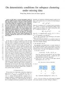
In the present section we derive a combinatorial formulation of the maximum split clustering problem under connectivity constraints; furthermore, we collect some theoretical properties which provide a basis for the algorithms to be discussed in Sections 4 to 7. The reader who is primarily interested in clustering applications may skip all proofs in this section. The length or weight of an edge {vk , v` } of G is defined to be the dissimilarity dk` between entities Ok and O` . Let T = (V, E(T )) be a spanning tree of G with minimal total length (i.e., a minimum spanning tree). Proposition 1 The split of an arbitrary partition (connected or not) of V is always equal to the length of some edge of T . Proof: See Rosenstiehl (1967), Delattre and Hansen (1980). Notice that, while a minimum spanning tree T is not necessarily unique (unless all dissimilarity values are different), the list S of lengths of the edges of T is unique. We define S ≡ [s1 , s2 , . . . , sN −1 ], where sj is the length of the j th shortest edge of T . Remark 2. It is possible that, for some s ∈ S, there is no connected partition of H whose split is equal to s, as shown by the following example. Example 1. Let D be the dissimilarity matrix of Table 1 and let H be the graph of Figure 1. A minimum spanning tree T of G is shown in Figure 2. Here S = [1, 2, 2, 3, 4], and one can check that there is no connected partition of H with split 3. Indeed, 7

1 2 3 4 5 6

1 0 3 4 6 1 8

2 3 0 5 2 4 3

3 4 5 0 9 4 7

4 6 2 9 0 2 4

5 1 4 4 2 0 6

6 8 3 7 4 6 0

Table 1: Dissimilarities (associated with edges of G)

v3

v2 v1

v4 v6

v5

Figure 1: Contiguity graph H of Example 1

v2

v3

v1

v4 v5

v6

Figure 2: Minimum spanning tree T of G for Example 1 entities O1 and O5 must belong to the same cluster since d15 = 1. This entails that entity O6 must belong to the same cluster than O1 and O5 to satisfy the connectivity constraints as vertex v6 belongs to all paths linking v1 to v5 (note that it is an articulation point of graph H). Finally entities O2 , O4 and O5 must be in the same cluster since d24 = 2 = d45 . The resulting partition {{v1 , v2 , v4 , v5 , v6 }, {v3 }} has a split equal to 4. n

For a given s ∈ S, let Gs be the graph (V, E(Gs )) where E(Gs ) ≡ {vk , v` } ∈ o

E(G) : dk` < s . Starting from any given minimum spanning tree T of G, define Ts 8

n

o

in a similar way, i.e., E(Ts ) ≡ {vk , v` } ∈ E(T ) : dk` < s . Observe that Ts is a spanning forest of Gs . Proposition 2 A partition PM has split at least s if and only if for every edge {vk , v` } of Ts , both vk and v` belong to the same cluster of PM . Proof: Clearly PM has split at least s if and only if each connected component of Gs is contained in some cluster of PM . Thus, in order to establish the proposition, it will be enough to prove that Gs and Ts have the same connected components. Since E(Ts ) ⊆ E(Gs ), every connected component of Ts is contained in some connected component of Gs . Conversely, let γ be a path in Gs joining vk and v` . We shall exploit the fact that one can always build the minimum spanning tree Ts via Kruskal’s (1956) greedy algorithm. This algorithm, starting from E = ∅, selects, at each iteration, the shortest edge e which has not been previously examined and then inserts e into E, unless e forms a cycle together with the other edges of E. At the end, one has E = E(T ). Right after all edges {vk0 , v`0 } such that dk0 `0 < s have been examined, one has E = E(Ts ). If e is any edge of γ, then either e ∈ E(Ts ) or e joins two vertices in a same connected component of Ts . It follows that vk and v` belong to the same connected component of Ts . The next definition leads to a purely combinatorial reformulation of connected max split graph clustering. Definition 1 If F and F 0 are two forests having the same set of vertices, F wraps F 0 if each connected component of F 0 is (vertex wise) contained in some connected component of F . Next, we introduce the following combinatorial problem: forest wrapping Given a (connected) graph H, a forest B having the same vertex set as H and an integer M , 1 < M < N , is there a spanning forest F of H having at least M connected components and such that F wraps B ? Proposition 3 connected max split graph clustering is reducible to forest wrapping. 9

Proof: Given a yes-instance of connected max split graph clustering, define j B to be Ts . Let PM = {C1 , . . . , CM } ∈ ΠC M (H). Let T be a spanning tree of the connected graph H(Cj ), j = 1, . . . , M , and let F be the spanning forest whose set of edges is E(T 1 ) ∪ E(T 2 ) ∪ . . . ∪ E(T M ). By Proposition 2, any two vertices in the same connected component of Ts belong to the same cluster Cj of PM , and hence to the same tree T j . Hence, F wraps B. Conversely, assume that F is a spanning forest of H which wraps B and has at least M connected components V1 , . . . , VM 0 . Then PM 0 = {V1 , . . . VM 0 } is a connected partition and its split is at least s. Notice that, when B has only one non-singleton connected component, forest wrapping essentially becomes the Steiner problem on a graph. For s ∈ S, define m(s) to be the maximum number of clusters in a connected partition whose split is at least s, i.e., the maximum number of connected components in a spanning forest F of H which wraps Ts . Note that F has m(s) connected components if and only if F has the smallest number of edges among the spanning forests wrapping Ts . Proposition 4 For every M , 1 ≤ M ≤ m(s), there is a PM ∈ ΠC M (H) whose split is at least s. Proof: Let Pm(s) ∈ ΠC m(s) (H). Since H is connected, there must be, in Pm(s) , two clusters Ci and Cj which are adjacent (i.e., there is an edge of H having one endpoint in Ci and the other one in Cj ). Merging Ci and Cj into a single cluster, one obtains a connected partition with m(s) − 1 components and with split at least s. Iterating this procedure, one obtains the desired result. Notice that the connectivity of H plays an crucial role here. We shall denote by F (s) a spanning forest of H which wraps Ts and has the smallest number of edges (briefly, an optimal forest). For a given s ∈ S, let K1 , . . . , Kq be the connected components of Ts : K1 , . . . , Kq define subsets whose vertices must be in a same connected component of F (s). The next result allows us to merge some of these subsets: Proposition 5 Let Ki and Kj be two connected components of Ts . If there exist 2 vertices u, v ∈ Ki that are disconnected in the subgraph of H induced by the set of vertices V \ V (Kj ), then the vertices of Ki and Kj must be in a same connected component of F (s). 10

Proof: Since u and v belong to the same connected component of Ts , they must be in the same cluster in PM . Let C be the connected component of F (s) that contains u and v. By definition, there exists a path γ between u and v, with all vertices of γ in C. By assumption, this path contains a vertex of Kj . Since all vertices of Kj must be in the same component, it follows that C contains Kj . Each time we merge two subsets Ki and Kj , we add an edge in Ts between one arbitrary vertex of Ki and one arbitrary vertex of Kj , so that the resulting merged subset is still a connected component of a forest. We denote this forest by Ts0 . Observe that Proposition 5 remains valid for Ts0 . The next result allows one to pinpoint a set Q of edges which must certainly be contained in some F (s), thereby reducing the computational effort required to find F (s). Let K1 , . . . , Kq be the connected components of Ts0 . Let F i be a maximal q

spanning forest of H(Ki ). Let Q = ∪ E(F i ). i=1

Proposition 6 There always exists an optimal forest F (s) whose set of edges contains Q.





Proof: Let F (s) be an arbitrary optimal forest. Assume that Q ∩ E F (s) = t, 



where 0 ≤ t < |Q|. Consider an arbitrary edge e = {vk , v` } ∈ Q \ E F (s) . Since vk , v` belong to the same connected component of Ts0 and since F (s) wraps Ts0 , there must be a path γ in F (s) joining vk to v` . At least one of the edges e0 along γ must  belong to E F (s) \ Q, otherwise the edges of γ together with e would form a cycle contained in Q, which is impossible. By replacing e0 by e one obtains a spanning forest F 0 (s) which has the same number of edges as F (s) and still wraps Ts0 . Fur thermore, one has Q ∩ E F 0 (s) = t + 1. Iterating this procedure one obtains the desired result. We next mention a corollary of a result of Simeone (1978) which specifies a family of subgraphs of H containing or giving an optimal solution. ˆ of H such that the optimal solutions Proposition 7 There exists a spanning tree H ˆ coincide. of connected max split graph clustering for H and H 11

Proof: See Maravalle and Simeone (1995). In fact the result of Maravalle and Simeone (1995) is much more general than Proposition 7, as it applies to connectivity constrained clustering with any criterion which does not depend of the graph H. However, the proof of this result is not constructive. Finally, let us discuss some consequences of the results of this section. Since the objective function of the maximum split clustering problem under connectivity constraints is of the bottleneck type (max-min), it is natural to think of a threshold algorithm for its solution: namely, given a certain threshold parameter s, such an algorithm would try to find a connected partition whose split is at least s and having a prescribed (or a maximum) number of clusters. Proposition 1 says that it is always sufficient to consider at most N − 1 special values of the threshold s, which are easily obtainable via a minimum spanning tree computation. Proposition 2 provides an efficient way to check that the split of a given partition is at least s. Proposition 3 provides a purely combinatorial formulation, i.e., forest wrapping, of connected max split graph clustering. In Section 6 we shall investigate this formulation to develop an exact algorithm for the latter problem. Proposition 4 implies that, once a connected partition with split at least s and having the maximum number of clusters has been found, it is quite easy to find a connected partition whose split is at least s and having any prescribed smaller number of clusters. Finally, Propositions 5 and 6 enable us to simplify the problem by showing that certain edges must be present in some or in all optimal forests. The above considerations lead to the algorithms described in the next sections.

4

Maximum split clustering on trees

As mentioned in the introduction, the particular case of connected max split graph clustering where the connectivity graph H is a tree has been studied by Maravalle and Simeone (1985), Maravalle, Simeone and Naldini (1997). They provide an O(N 3 ) algorithm to solve it. We next present an algorithm whose worst case complexity is Θ(N 2 ). When H is a tree, by deleting (or “cutting”) M − 1 edges of H but not their endpoints, one obtains a forest with M components, and these components are the 12

clusters of a connected M -partition. Conversely, all connected M -partitions arise in this way. The algorithm ctree described below scans the edges of a minimum spanning tree T of G in non-decreasing order of lengths, s1 ≤ s2 ≤ · · · ≤ sN −1 (ties are broken arbitrarily). Let {vk , v` } be the current edge and let si = dk` . If we want to obtain a connected partition with split > si , then vk and v` must belong to the same cluster Cj . This implies that no edge along the unique path γ of H joining vk and v` must be cut. Hence, all vertices along γ must belong to Cj . The algorithm shrinks all these vertices into a single vertex in order to prevent edges along γ from being cut. We denote by C(vk ) the cluster of the current partition which contains Ok . Algorithm CTREE Step 1. Initialization Compute a minimum spanning tree T of G = (V, E(G)) Rank the edges {vk , v` } of T in non-decreasing order of dk` ; Ck = C(vk ) ← {Ok } for k = 1, 2, ..., N ; PN = {C1 , C2 , ..., CN } (PN is the granular partition in which all clusters are singleˆ ← H; M ← N ; tons); H Step 2. Path shrinking For i = 1, 2, . . . , N − 1 do Let {vk , v` } be the ith edge of T ; If C(vk ) 6= C(v` ) then ˆ Let γ be the (unique) path joining C(vk ) and C(v` ) in H; Let M 0 be the number of vertices of γ (vk and v` excluded); M ← M − M 0 − 1; For each vertex v of γ, merge C(v) with C(vk ); Shrink all vertices of γ into a single vertex; ˆ accordingly; Update H EndIf Output the (connected) partition PM of H EndFor. Theorem 2 Let s ∈ S. Right after all edges of T with length smaller than s have been processed, the current partition P is a connected partition of H with split at least s and with a maximum number of clusters. 13

Proof: The result is a consequence of the following two remarks: (i) For every pair of vertices vk , v` such that {vk , v` } ∈ E(T ) and dk` < s, no edge along the path γ of T joining vk and v` is cut in P . This follows from the fact that, when edge {vk , v` } is processed, all vertices of γ are shrunk into a single vertex. Notice that some of them might have been shrunk during previous iterations. (ii) All edges of H are cut in P , except for those specified in (i). In view of Proposition 2, (i) implies that s(P ) ≥ s. Moreover, the partition P is connected by construction. Finally, (ii) implies that P has a maximum number of clusters among all connected partitions with split at least s, since all such partitions must satisfy (i) anyhow. Algorithm ctree can be implemented so as to run in O(N 2 ) time. Actually, computing a minimum spanning tree of the (complete) graph G already takes O(N 2 ) time. Reading the dissimilarity matrix requires Ω(N 2 ) time: thus the algorithm has a complexity in Θ(N 2 ), i.e., it is the best possible. Note that the partition output by the algorithm has a split at least s, which means that the split may be actually greater. It follows that the algorithm may produce several partitions with the same split but with a different number of clusters. In that case, the partition that is generally considered the most interesting is the one with the largest number of clusters.

5

Some heuristics for general graphs

ˆ Algorithm ctree iteratively merges the vertices of the unique path γ of the tree H ˆ corresponding to the endpoints of the edge (vk , v` ) of T between the vertices of H ˆ This observation under consideration. Such a path is of course a shortest one in H. suggests a simple modification to be given to ctree, in order to obtain a heuristic, called htree, for the general case. It suffices to specify that at each iteration one seeks ˆ Otherwise, a shortest path γ between the vertices corresponding to vk and v` in H. the rules are the same. Such an algorithm is called a greedy one because it optimizes some criterion (here minimization of the reduction in number of clusters) at each 14

iteration in a myopic way. So after a few iterations one may obtain partitions whose split is at least s for which the number of clusters is not the largest possible. The complexity of htree is in O(N 3 ). Example 2. Consider the graph H of Figure 3 and any dissimilarity matrix where d26 = 3, d68 = d79 = 5, d19 = 8, and all remaining dissimilarities are greater than or equal to 8. Then S = [3, 5, 5, 8, . . .]. Choose s = 8. The edges of T8 are {v2 , v6 }, {v6 , v8 }, {v7 , v9 }. v2

e2

e1

e5 v3

e4

v5

e6

v6 e7

v4

e3

v7 e10

v1

e11

v9

e9

e8 v8

v10

Figure 3: Contiguity graph of Example 2. The heuristic htree finds the connected partition with 3 clusters shown in Figure 4, while a connected partition with a maximum number of clusters (i.e., 4) is shown in Figure 5. v2

v5 v3

v6

v4

v7

v1

v9

v8

v10

Figure 4: Partition found by htree (s ≥ 8)

15

v2

v5 v3

v6

v4

v7

v1

v9

v8

v10

Figure 5: Optimal partition with maximum number of clusters (s ≥ 8) As mentioned above, algorithm htree proceeds in a myopic way; moreover, there may be arbitrary choices to make if, at a given iteration, there are several shortest paths between the vertices vk and v` in H. Another way to obtain a heuristic, based on ctree for the case where H is a general graph, which avoids the second drawback, is to select some spanning tree TH of H and then apply ctree to it. Proposition 7 provides motivation to do so. One criterion for selecting edges to belong to this tree is that they belong to shortest paths between endpoints vk and v` of edges of T . This idea can be implemented as follows: Heuristic pathtree Step 1. Minimum spanning tree Compute a minimum spanning tree T of G = (V, E(G)) Step 2. Weighting edges Weight the edges {vi , vj } of H by the number of edges {vk , v` } of T such that {vi , vj } belongs to a shortest path between vk and v` ; Step 3. Maximum spanning tree Find a maximum spanning tree TH of H with the weights so defined; Step 4. Path shrinking Apply ctree to TH . The complexity of heuristic pathtree is in O(N 3 ), due to Step 2. Focusing on the dissimilarity matrix D = (dk` ) suggests another, simpler way to obtain a spanning tree TH : 16

Heuristic distree Step 1. Weighting edges Weight the edges of H by the corresponding dissimilarities; Step 2. Minimum spanning tree Find a minimum spanning tree TH of H with the weights so defined; Step 3. Shrinking edges Apply ctree to TH . This heuristic has a complexity in Θ(N 2 ). Algorithm distree is similar to the first steps of the midas algorithm of Maravalle and Simeone (1995) for connected partitioning with the minimum inertia criterion (the latter algorithm also includes rules for improvement by tree-modification). The first two steps of distree are also the same as those of the algorithm of Monestiez (1977) discussed above; the third one is different as ctree, which exploits all dissimilarities, is then used instead of Gower and Ross’ (1969) single linkage algorithm. The three heuristics described in this section, as well as another one (derived from the exact algorithm) presented in Section 7 are compared experimentally in Section 8.

6

An exact algorithm for general graphs

In the present section we describe an iterative exact algorithm for solving the connected max split graph clustering problem on a general graph. An informal description is given in Section 6.1. A formal description follows in Section 6.2. Some discussion on the number of iterations can be found in Section 6.3.

6.1

Informal description

As seen in Section 3, the problem can be reformulated as follows: 

(P )

Given s ∈ S, find a spanning forest F of H which wraps Ts0 and has the smallest number of edges.

The algorithm proposed below finds a solution to (P ) by solving a sequence of increasingly constrained set covering problems. The basic idea is the following. Let 17

K1 , . . . , Kq be the connected components of Ts0 . Let Ki be one such component with cardinality ≥ 2 and let vk , v` ∈ Ki , vk 6= v` . Consider now an arbitrary subset Vk` of V which contains vk but not v` . We denote by Vk` the collection of all such subsets Vk` . Let ω(Vk` , v` ) be the subset of edges {u, v} of H with u ∈ Vk` and v 6∈ Vk` such that there exists a path from v to v` not going through any vertex from Vk` . Since an optimal forest F wraps Ts0 , there must be a path γ in F joining vk to v` . At least one of the edges of γ must belong to ω(Vk` , v` ). To enforce this we write down the constraint X xe ≥ 1, e∈ω(Vk` ,v` )

where



xe =

1 if e ∈ F, 0 otherwise.

Hence, we can write down the following set covering problem, later called the master set covering problem

(MSC)

P  min xe    e∈E(H)    subject to: P  xe ≥ 1,    e∈ω(Vk` ,v` )  

xe ∈ {0, 1},

i = 1, . . . , q; vk , v` ∈ Ki ; Vk` ∈ Vk`

e ∈ E(H).

Any optimal solution to (MSC) must be a spanning forest of H wrapping Ts0 and having a minimum number of edges. The set covering problem (MSC) has only m = |E(H)| variables but a huge number of constraints. Thus it is usually computationally infeasible to solve (MSC). Hence, we shall take a constraint generation (or cutting plane) approach: instead of solving (MSC) directly, we solve a nested sequence of set covering problems, the rth of which involves a (usually small) subset Lr of constraints of (MSC), with L1 ⊆ L2 ⊆ · · ·. An optimal solution to Lr yields a spanning forest Fr . If Fr wraps Ts0 then Fr is an optimal solution to problem (P ); if not, for each pair of vertices (vk , v` ) such that vk and v` belong to the same connected component of Ts0 but to two different connected components Ci = Vk` and Cj = V`k of Fr , add to Lr the constraints corresponding to ω(Ci , v` ) and ω(Cj , vk ). Observe that these constraints are present in (MSC) but are absent from Lr , since they are violated by the optimal solution of the rth set covering 18

problem. Call Lr+1 the resulting set of constraints and iterate. Note that a same set covering constraint can be obtained for different ω(C, v): in that case of course, we generate the constraint only once. In order to initialize the procedure, one takes F0 to be the forest whose connected components are the single vertices of V . Clearly the algorithm is finite since new constraints are added at each iteration and the total number of constraints is bounded from above by N 2N . Example 3. Consider again Example 2, with s = 8. F0 is the forest consisting of the 10 isolated vertices. The initial set L1 of constraints is x1 + x2 x6 + x7 x7 + x8 x8 + x9 x9 + x10

≥ ≥ ≥ ≥ ≥

1 1 1 1 1

(ω({v2 }, v6 )) (ω({v6 }, v2 ) and ω({v6 }, v8 )) (ω({v7 }, v9 )) (ω({v8 }, v6 )) (ω({v9 }, v7 ))

(note that in the last constraint, the variable x11 does not appear because the only path from v10 to v7 passes through v9 ). One optimal solution to the first set covering problem corresponds to the forest F1 whose set of edges is {e1 , e7 , e9 }. The connected components of F1 are {v1 , v2 }, {v3 }, {v4 }, {v5 }, {v6 , v7 }, {v8 , v9 }, {v10 }. Notice that v2 and v6 belong to different components of F1 , and so do v6 and v8 , and v7 and v9 . Hence, one obtains L2 by adding to L1 the constraints x2 + x3 ≥ 1 (ω({v1 , v2 }, v6 )) x6 + x8 ≥ 1 (ω({v6 , v7 }, vi ) for i = 2, 8, 9) x8 + x10 ≥ 1 (ω({v8 , v9 }, v6 ) and ω({v8 , v9 }, v7 )). An optimal solution F2 to the second set covering problem corresponds to the set of edges {e2 , e6 , e8 , e10 }. One obtains L3 by adding to L2 the constraints x4 ≥ 1 x5 + x7 ≥ 1 x7 + x9 ≥ 1 x5 + x9 ≥ 1. An optimal solution F3 corresponds to {e2 , e4 , e7 , e8 , e9 }. One obtains L4 by adding the constraints x5 + x10 ≥ 1 x6 + x10 ≥ 1. 19

An optimal solution F4 corresponds to {e2 , e4 , e7 , e8 , e9 , e10 }. This time F4 wraps T8 . Thus, F4 yields an optimal forest for s = 8. (One sees that F4 coincides with the forest shown in Figure 5.) One possible refinement of the algorithm is to use Propositions 5 and 6 to detect edges which must be present in an optimal forest F (s). This is done by replacing Ts by Ts0 . Example 4. Consider again Example 2, with s = 8. At the beginning, the connected components of T80 = T8 are {v1 }, {v2 , v6 , v8 }, {v3 }, {v4 }, {v5 }, {v7 , v9 } and {v10 }. Applying two times Proposition 5 shows that v3 and v4 must be in the same cluster than v2 , which we can express by adding to T8 the edges {v2 , v3 } and {v2 , v4 }, obtaining the new forest T80 . The connected components of T80 are K1 = {v1 }, K2 = {v2 , v3 , v4 , v6 , v8 }, K3 = {v7 , v9 }, K4 = {v5 }, K5 = {v10 }. Since all paths in H from v7 to v9 pass through a vertex from K2 , we can merge K2 and K3 by Proposition 5. The edges of a maximal spanning forest of the subgraph H(K2 ∪ K3 ) induced by K2 ∪ K3 are e3 , e4 , e7 , e8 , e9 . All these edges must be present in an optimal forest F (8) by Proposition 6. The set of edges of the initial spanning forest F0 is E 1 = {e3 , e4 , e7 , e8 , e9 }. Hence the connected components of F0 are {v2 , v3 , v4 }, {v5 }, {v6 , v7 , v8 , v9 } and {v10 }. The initial set L1 of constraints is x5 + x10 ≥ 1

(e.g., ω({v2 , v3 , v4 }, v6 ))

x6 + x10 ≥ 1

(e.g., ω({v6 , v7 , v8 , v9 }, v2 )).

The optimal solution of the set covering problem consists of the edge e10 . The forest F1 consisting of ne10 and of the edges of E1 wraps T8 and hence it is an optimal F (8). o Therefore P4 = {v1 }, {v2 , v3 , v4 , v6 , v7 , v8 , v9 }, {v5 }, {v10 } is a connected partition with split at least 8 and having the maximum number of clusters. A further refinement of the exact algorithm consists in finding suboptimal — rather than optimal — solutions to the set covering problems by means of some fast heuristic, as long as new constraints are generated. As soon as a suboptimal solution of some set covering problem yields a wrapping forest (possibly not having a minimum number of edges), this problem is solved again, but this time up to optimality i.e., by an exact algorithm. Notice, however, that the optimal solution of the covering problem so obtained may not correspond to a wrapping forest. In this case the algorithm goes on, solving again heuristically and then exactly set covering problems until the exact algorithm yields a solution which corresponds to a wrapping forest.

20

6.2

Formal description

We now give a formal description of the full version of the algorithm. Algorithm ccmsc Step 1: (Initialization) Compute a minimum spanning tree T of G with respect to lengths of the edges given by the dissimilarities; S ← list of lengths of the edges of T , sorted in non-decreasing order; s ← first value of S; Ts ← G(V, ∅) Step 2: (Preprocessing) Use Proposition 5 to compute the forest Ts0 ; Use Proposition 6 to compute a set of edges E 1 that must be present in an optimal forest F (s); Let F be the forest (V, E 1 ); heur ← false;  X  xe  min 1 Let SC be the trivial set covering problem e∈E(H)\E   s.t. xe ∈ {0, 1}, e ∈ E(H) \ E 1 ; Step 3 (Wrapping test and constraint generation) For all {vk , v` } in a same connected component of Ts0 do If vk , v` belong to 2 different connected components C 0 , C 00 of FXthen X Update SC by adding the constraints xe ≥ 1 and xe ≥ 1; e∈ω(C 0 ,v` )

e∈ω(C 00 ,vk )

EndIf EndFor; If no constraint has been added then go to 5; Step 4: (Heuristic solution of set covering subproblem) heur ← true; Find a suboptimal solution x˜ to SC by a heuristic; Let F be the forest whose set of edges is E 1 ∪ {e ∈ E(H) : x˜e = 1}; Go to 3; Step 5: (Optimality test) If heur = false then go to 7

{an optimal forest F (s) has been found};

Step 6: (Exact solution of set covering subproblem) heur ← false 21

Find an optimal solution x∗ to SC; Let F be the forest whose set of edges is E 1 ∪ {e ∈ E(H) : x∗e = 1}; Go to 3; Step 7: (Output optimal partition) M ← N − |E(F )|; Let PM be the connected partition whose M clusters are the connected components of F ; { in general s(PM ) ≥ s}; Output s, M, PM , s(PM ); Step 8: Next split value Let s be the smallest value in S satisfying s > s(PM ); If s does not exist then stop; n o Let Ts be the forest {V, E(Ts )} with E(Ts ) = {vk , v` } ∈ E(T ) | dk` < s ; Go to 2. Note that in Step 8, we can start from the tree Ts00 obtained for the value s00 of the previous iteration and add the edges {vk , v` } such that s00 ≤ dk` < s. Similarly, in Step 2, the preprocessing can be somewhat sped up by considering only the changes brought by the new edges. Observe that the ccmsc algorithm usually provides optimal partitions for some values of M but not for all; in other words, only some of the values of the split s ∈ S correspond to optimal partitions under connectivity constraints with a maximum number of clusters. For some applications, it may be desirable to find partitions with a given number M of connected clusters and the largest possible split under such conditions. One may proceed as follows. First, compute the split s of the partition with M clusters using the single linkage algorithm (s is equal to the (M − 1)th value of S). Next, apply the ccmsc algorithm with S = {s}. The variant of the ccmsc algorithm so obtained will be denoted ccmsc(s). Let M 0 denote the number of clusters obtained. If M 0 < M , apply ccmsc(s0 ) algorithm where s0 is equal to the largest value of S smaller than s. Repeat the process until M 0 ≥ M . If M 0 > M , use Proposition 4 to merge clusters until M 0 = M (note that this merging step cannot result in an increase of the split).

6.3

Remark on the complexity of the algorithm

The ccmsc algorithm has to solve repeatedly set covering problems, which are NPhard. In this section, we show that it is even not possible in general to bound the 22

number of set covering problems to solve by a polynomial in N (or equivalently the number of constraints in the last solved set covering problem). Let us consider the graph H drawn in Figure 6 with N = p2 + 2. Assume

v1 e1

e2 e e 3 e5 4 v2

v3

v4

e6

ep

v5

v6

v7

vp+2

vp+1 v2p+1

vp2+1

vN Figure 6: Contiguity graph H that the dissimilarity between vertices v1 and vN is 1, that the dissimilarity between vertices v1 and v2 is 2 and that the other dissimilarities are ≥ 2. For simplicity we assume that all set covering problems are solved exactly (this is for example the case if the heuristic is very good). For the first threshold split value s = 1, the algorithm finds the granular partition with N clusters, with split equal to 1. The next value in S is s = 2. The forest Ts0 = Ts is reduced to the edge {v1 , vN }, F is the forest composed of the N isolated vertices and E 1 = ∅. Since {v1 , vN } belongs to Ts0 but v1 and vN are in different connected components of F , we add the following constraints to the set covering problem in Step 3: x1 + . . . + xp ≥ 1 x|E(H)|−p+1 + . . . + x|E(H)| ≥ 1. 23

Observe that since we are minimizing

|E(H)| P

xi , any variable not appearing in the con-

i=1

straints will be at 0 in any optimal solution. Observe furthermore that when we add set covering constraints, new variables can be introduced only when the corresponding edge is incident to an edge whose variable was at 1 in the optimal solution of the previously solved set covering problem. This implies that at least during a certain number of iterations, the constraints of the set covering problems can be partitioned in two groups: one involving variables corresponding to edges that are close to v1 , and the other one involving variables corresponding to edges close to vN . The set covering problems themselves can be decomposed accordingly. From now on, we focus on the partial set covering problems associated to v1 . A subgraph of H is said to be a v1 -rooted subtree if it is a tree containing the vertex v1 . Given a graph G, the v1 -connected component of G is the connected component of G containing v1 . Note that a given set of vertices can be the v1 connected component vertex set of more than one v1 -rooted subtree. We first need the following Lemma: Lemma 1 As long as the set covering constraints associated to v1 and vN do not include common variables, the ccmsc algorithm generates a sequence of blocks Bv(1) , Bv(2) , . . . , Bv(k) ,... 1 1 1 of subgraphs of H, where: a) each block Bv(k) contains v1 -rooted subtrees of H with exactly k edges; 1 b) all v1 -rooted trees of Bv(k) have a different v1 -connected component vertex set; 1 c) for each possible v1 -connected component vertex set with k + 1 vertices, there exists in Bv(k) a v1 -rooted tree with this v1 -connected component vertex set. 1 The order in which the trees appear in a particular block is not relevant. Proof: Since the set covering constraints are added at each iteration, the sequence of optimal values is non-decreasing, hence the sequence of solutions generated has the block-structure indicated in the Lemma. Note also that since the set covering constraints are defined with respect to the connected component vertex set of the current v1 -rooted subtree, we cannot generate two subtrees with the same connected component vertex set: this shows the point b). It remains to show that 1) no subgraph of H other than trees containing v1 can be generated and that 2) for all v1 -connected component vertex set of size k + 1, a v1 -rooted subtree is generated. We proceed by induction on k. The property is true for k = 1: at the beginning, the set covering problem (recall that we consider only the part corresponding to v1 ) contains 24

the unique constraint x1 + . . . + xp ≥ 1

(1)

expressing that at least one edge leaving v1 must be chosen. An optimal solution of this set covering problem is obtained by fixing an arbitrary xi to 1. The new set covering constraint that is added is then of the form p X j=1,j6=i

xj +

X

xe ≥ 1.

e∈E(H):e={vi+1 ,v},v6=vi

Again an optimal solution is obtained by fixing a variable x` to 1 (note however that we must have ` 6= i, otherwise the just introduced constraint would be violated). Using the same reasoning, we see that the algorithm enumerates the p solutions of value 1. Each of these solutions corresponds to a v1 -rooted subtree of H of size 1. No other solution of value 1 can be obtained, since it would violate the constraint (1). Moreover with each v1 -connected component of 2 vertices we can associate a v1 -subtree. Now assume that the property is true up to k. We want to show that it is still true up to k +1. Assume first that a subgraph G of H that is not a v1 -rooted tree is generated. By the nature of the set covering constraints, G must be a forest, otherwise we could strictly improve the solution by removing one of the edges of a cycle. Consider now the connected component G0 of G containing v1 : G0 is a v1 -rooted subtree of H of size ≤ k. By the induction assumption, the set covering problem contains a constraint relative to G0 (or more precisely, to its v1 -connected component vertex set). Clearly this constraint is violated by G, which shows that only v1 -rooted subtrees of H can be generated. Now assume that there exists a v1 -connected component vertex set S of H, with k + 2 vertices, that violates the set covering constraint associated with a v1 -connected component vertex set S 0 of size ≤ k + 2 previously generated. We show that this leads to a contradiction. Since |S| ≥ |S 0 | and S 0 6= S, we cannot have S ⊆ S 0 , hence there exists a vertex u ∈ S \ S 0 . Since S is v1 -connected, there exists a path in H joining v1 to u. But this path necessarily contains an edge joining a vertex of S 0 to a vertex of S \ S 0 , hence the set covering constraint corresponding to S 0 is satisfied, a contradiction. Therefore all v1 -connected component vertex sets of size k + 2 will be generated, which completes the proof. Proposition 8 The ccmsc algorithm can take a super-polynomial number of iterations on some instances. 25

Proof: Consider again the graph H of Figure 6. By Lemma 1, the algorithm enumerates all v1 -connected component vertex sets of the graph H in increasing order of size. The shortest path between v1 and vN has length p + 1, hence there is still no interference between the partial set covering problems corresponding to v1 and those corresponding to vN when the algorithm enumerates the v1 -connected component   vertex sets with b p2 c + 1 vertices. This gives a lower bound of b pp c on the number 2 of iterations, which corresponds to the number of the v1 -connected component vertex √ sets with vertices in {v2 , . . . , vp+1 } (in addition of the vertex v1 ). Since p = O( N ), the result follows. Remark 3. The above result also holds for more general graphs and for more general dissimilarity distributions. In particular, all what is needed in the proof of Proposition 8 is that the graph H satisfies the following properties: √ • v1 has at least p neighbours v2 , . . . , vp+1 , with p = O( N ), such that from each of these vertices there exists a path to vN not passing through v1 ; • There exists at least 2 vertex-independent paths between v1 and vN (this ensures that no preprocessing due to Proposition 5 occurs in Step 2); • The shortest path between v1 and vN has length ≥ p + 1. Note also that Proposition 8 is still true if instead of√considering v1 -connected comv1 -connected ponent vertex sets with b p2 c + 1 vertices with p = O( N ),we consider  1 p component vertex sets with b c c + 1 vertices with p = O N c0 where c and c0 are integer constants ≥ 2. Finally there may be more than one dissimilarity with value 1. The simplest way to obtain such an instance is to consider c00 copies of H, where c00 is a constant, and merge the vertices v1 of each copy together in order to obtain a connected graph.

7

Another heuristic for general graphs

Exact solution of the set covering subproblems is by far the most time-consuming part of the ccmsc algorithm. Quite often the heuristic of Step 4 is sufficient to find an optimal solution and Step 6 only aims at proving optimality of this solution. When large instances or dense contiguity graphs H are considered, computing time necessary for exact solution becomes prohibitive. Then another heuristic for connected max 26

split graph clustering is obtained by only solving heuristically the set covering problems. Modifications to be made to the ccmsc algorithm are: (i) deletion of Steps 5 and 6 and (ii) move to Step 7 instead of Step 5 when Step 3 shows a wrapping has been obtained. We call hcover the heuristic obtained in this way. The set covering algorithm used in ccmsc and hcover is close to that of Fisher and Kedia (1990). We used the primal heuristic and the first and third dual heuristics that they proposed.

8

Computational experience

All heuristic algorithms (htree, pathtree, distree, hcover) as well as the exact ccmsc algorithm for general graphs proposed in this paper have been tested on a sun Enterprise-10000 computer (400 Mhz, 64 G). Seven test problems have been considered. The first five of them (tuscany, rome, campany, latium, upper latium) are regional clustering problems from Maravalle and Simeone (1995). Their characteristics are recalled in Table 2. The graph H expresses contiguity between

Test problem

N

tuscany rome campany latium upper latium paris usa

287 121 81 412 210 90 48

|E(H)| density = 773 302 165 566 331 444 212

|E(H)| N

# characteristics

2.69 2.50 2.04 1.37 1.58 4.93 4.42

1 1 6 1 5 -

Table 2: Characteristics of the test problems districts in the city for the rome problem. For the other four problems, the vertices represent towns and the edges represent major roads between towns. Thus all graphs are planar or nearly planar. Dissimilarities are Euclidean distances between measurements of 1 to 6 socio-economic characteristics. Two additional test problems (paris, usa) have been constructed. For the paris problem, the entities correspond

27

to the districts of Paris and its surroundings. The graph H represents the contiguity between districts. For the usa problem, the entities correspond to the states of usa and the graph H represents the contiguity between states (the states Hawai and Alaska were removed in order to have a connected graph). For these four problems, the dissimilarity values are drawn at random in a uniform distribution on the interval [0, 1]. The dissimilarity matrices and the contiguity graphs for all these 7 instances are available on the web site www.crt.umontreal.ca/∼sphinx1. The remaining of this section is organized as follows. In Section 8.1, we compare the performance of the four heuristics for all values of the threshold split on the Campany instance. In Section 8.2, we do a similar analysis for the other instances but for a small subset of the threshold values. Finally in Section 8.3, we consider the variant of the exact ccmsc algorithm that gives a partition with the largest possible split for a specified number of clusters.

8.1

Heuristic solution of Campany for all values of the threshold

We first solved the Campany instance for all values of the threshold split by the four heuristics (recall that the threshold values are considered in increasing order). The computing times (in seconds) were the following: htree: 0.05s, pathtree: 0.14s, distree: 0.04s, hcover: 1107182s (12 days 19 hours 33 minutes). The distribution of the time for hcover is given in Figure 7. We observe that the computing time is reasonable for roughly the 17 smallest threshold values and the 27 greatest values, but explodes for intermediate values. Since solving exactly campany was not possible, we evaluate the quality of the heuristics with respect to the best value found by the 4 heuristics. Figure 8 represents the difference with respect to the best value (i.e., the number of clusters), for each heuristic and for each value of the threshold. The best results are obtained by the htree and hcover heuristics. Heuristic distree performs particularly badly for the first half of the threshold values: this is due to the fact that the 2 clusters that have to be merged at the very beginning are connected together by a long path, and hence all clusters that are on this path must also be merged with the 2 clusters. Another way to look at the results of Figure 8 is given in Table 3, which gives for each heuristic the number of times the solution found was the best one, the second 28

120000

computing time (in seconds)

100000

80000

60000

40000

20000

0

0

10

20

30

40 50 index of the split threshold

60

70

80

Figure 7: Repartition of the computing time for hcover 25

htree distree pathtree hcover

relative # of clusters

20

15

10

5

0 0

10

20

30 40 50 index of the split threshold

60

70

Figure 8: Difference to the best value for the 4 heuristics 29

80

best one, the third best one, etc... Note that htree finds the best solution slightly more often than hcover does. However if we consider rank 1 and 2 together, hcover wins clearly, at least with respect to the quality of the solution found (hcover takes considerably much more time through). distree and pathtree are clearly outclassed. | htree | distree | pathtree | hcover ---------------------------------------------------1 | 47 | 8 | 3 | 45 2 | 19 | 22 | 13 | 33 3 | 14 | 23 | 41 | 2 4 | 0 | 27 | 23 | 0 Table 3: Number of times each rank is obtained for Campany Table 4 gives some more additional indicators for the first 10% smallest threshold values, the last 10%, and some intermediate values. For hcover, these indicators are defined as follows: merge1 is the number of merges starting from the canonical partition (i.e., the partition where each entity defines a cluster) in order to obtain Ts ; merge2 is the number of additional merges done using the preprocessing of Proposition 5 to obtain Ts0 ; iter is the number of iterations through Step 4 of the algorithm. This number also corresponds to the number of set covering problems solved. The indicators ncon and nvar represent respectively the number of constraints and varii 2 3 4 5 6 7 8 9 17 25 33 40 50 58 66 74 75 76 77 78 79 80

si

M

htree split

8.01 8.22 10.52 13.56 13.80 14.10 14.33 15.24 17.28 19.95 22.67 23.86 25.69 27.45 29.92 38.07 39.62 41.00 41.03 44.57 50.49 51.56

79 73 72 71 69 65 64 62 43 34 25 20 14 11 6 4 3 3 2 2 1 1

8.01 8.22 10.52 13.56 13.80 14.10 14.33 15.24 17.28 19.95 22.67 23.86 25.69 27.45 31.78 38.07 41.00 41.00 44.57 44.57 ∞ ∞

tcpu

0.05

pathtree M split

M

78 73 72 68 63 60 59 58 38 27 20 15 10 9 5 3 2 2 1 1 1 1

68 53 52 51 51 49 49 49 30 22 19 16 12 11 6 5 4 4 3 3 2 2

8.01 8.22 10.52 13.56 13.80 14.10 14.33 15.24 17.28 19.95 22.67 23.86 25.86 28.99 31.78 38.07 41.00 41.00 ∞ ∞ ∞ ∞ 0.14

distree split 8.01 8.22 10.52 13.80 13.80 15.24 15.24 15.24 17.28 19.95 22.67 23.86 26.59 27.67 37.94 38.07 41.00 41.00 44.57 44.57 51.56 51.56

M

split

merge1

79 72 71 70 69 62 64 63 41 27 22 23 17 15 10 7 6 5 3 3 2 2

8.01 8.22 10.52 13.56 13.80 14.33 14.33 15.24 17.28 19.95 23.25 23.86 25.69 27.45 31.78 38.07 39.62 41.00 44.57 44.57 51.56 51.56

1 2 3 4 5 6 7 8 16 24 32 41 49 57 65 73 74 75 76 77 78 79

hcover merge2 iter 0 0 0 0 0 0 0 0 0 0 0 4 8 5 5 1 1 1 2 1 1 0

3 60 60 60 27 44 21 31 123 533 572 102 35 18 1 0 0 0 0 0 0 0

ncon

nvar

tcpu

6 135 135 135 89 175 93 136 831 2896 3218 570 135 47 2 0 0 0 0 0 0 0

27 94 94 94 78 121 90 89 164 168 168 132 90 59 13 0 0 0 0 0 0 0

0.00 17.89 18.02 17.70 4.48 18.47 3.75 9.26 282.60 5229.28 6501.25 185.40 15.98 2.35 0.00 0.00 0.01 0.01 0.01 0.01 0.00 0.01

0.04

Table 4: Results of the heuristics for Campany (N = 81) 30

ables in the last set covering problem solved. Finally tcpu is the total computing time in seconds. We observe that for the largest values of the threshold, the preprocessing step is sufficient to solve the problem with hcover and the computing time is very small. For intermediate values of the threshold, when the preprocessing does not allow any reduction of the problem, hcover can take much more time than the other heuristics while giving a solution of poorer quality.

8.2

Heuristic solution of the other instances

In most practical applications, the partitions of interest are those with a relatively small number of clusters. Such partitions are obtained for the largest threshold values. Table 5 presents the results obtained by the heuristics on the other instances when seeking a partition with split at least equal to the ith threshold value si , for large i. A limit of 10 hours was set for each run. The sign > in the tcpu column means that the problem was not solved within that time. Since for the htree, pathtree and distree heuristics, the program gives in one run the results for all values of the threshold, the overall computing time is indicated in the last line for these heuristics. hcover almost always provide the best results, within a reasonable computing time. The most notable exception is for the Rome instance: for i = 98, hcover finds a partition with 12 clusters after more than 16000s, whereas htree was able to find a partition with 14 clusters in less than 1s. For i = 86 and i = 110, hcover is not even able to finish within the allowed computing time. hcover is also not able to solve the Paris2 instance for i = 64. Among the tree-based heuristics, htree generally gives the best results, except for Latium and Upper Latium where it is clearly beaten by distree.

31

pathtree M split

M

1.20 2.50 12.90 12.90 12.90 14.30 14.30 14.30 29.30 29.30 ∞ 0.66

31 13 4 4 4 3 3 3 2 2 1

1.20 2.50 12.90 12.90 12.90 14.30 14.30 14.30 29.30 29.30 ∞ 1.84

31 12 4 4 4 3 3 3 2 2 1

1.20 2.50 12.90 12.90 12.90 14.30 14.30 14.30 29.30 29.30 ∞ 0.47

23 14 4 4 4 3 3 2 2 2 2 1

2.63 5.12 12.91 12.91 12.91 16.98 16.98 43.66 43.66 43.66 43.66 ∞ 0.11

13 7 3 3 3 2 2 2 2 2 2 1

2.63 5.12 12.91 12.91 12.91 43.66 43.66 43.66 43.66 43.66 43.66 ∞ 0.30

12 5 4 4 4 3 3 2 2 2 2 1

2.63 6.19 12.91 12.91 12.91 16.98 16.98 43.66 43.66 43.66 43.66 ∞ 0.07

1.70 2.80 17.30 25.50 26.60 29.50 48.60 80.80 130.10 243.00 529.90 tcpu

21 14 2 2 2 2 2 2 2 2 1

1.70 3.10 243.00 243.00 243.00 243.00 243.00 243.00 243.00 243.00 ∞ 1.00

21 14 3 3 3 2 2 2 2 2 1

1.70 3.10 26.60 26.60 26.60 243.00 243.00 243.00 243.00 243.00 ∞ 2.66

25 18 6 6 6 5 4 4 3 3 2

1.70 3.10 26.60 26.60 26.60 29.50 80.80 80.80 243.00 243.00 529.90 0.99

169 190 201 202 203 204 205 206 207 208 209

4.84 14.01 33.99 48.14 54.26 56.97 57.93 103.73 239.85 246.92 780.07 tcpu

19 8 4 4 3 2 1 1 1 1 1

4.84 14.01 48.14 48.14 54.26 56.97 ∞ ∞ ∞ ∞ ∞ 0.26

15 4 2 2 2 2 1 1 1 1 1

4.84 14.01 56.97 56.97 56.97 56.97 ∞ ∞ ∞ ∞ ∞ 0.72

16 10 7 6 4 3 2 2 2 1 1

64 73 82 83 84 85 86 87 88 89

1.49 1.87 3.02 3.29 3.47 4.49 4.67 4.75 5.39 6.28 tcpu

13 11 9 8 7 6 5 4 3 2

1.49 1.87 3.29 3.29 3.47 4.49 4.67 4.78 5.39 6.28

10 7 4 4 3 2 2 1 1 1

1.49 1.97 3.29 3.29 3.47 4.67 4.67 ∞ ∞ ∞

3.74 3.97 5.95 6.14 6.30 6.70 tcpu

12 9 5 4 3 2

i

si

M

231 259 278 279 280 281 282 283 284 285 286

1.20 2.10 10.10 10.50 12.90 13.30 14.20 14.30 25.80 29.30 62.70 tcpu

32 13 4 4 4 3 3 3 2 2 1

86 98 110 112 113 114 115 116 117 118 119 120

2.63 5.12 9.20 12.56 12.91 15.59 16.98 17.29 20.78 23.38 43.66 70.28 tcpu

331 372 403 404 405 406 407 408 409 410 411

35 39 44 45 46 47

htree split

0.08

0.02

8 6 4 3 2 2

split

merge1

ncon

nvar

tcpu

Tuscany 35 15 5 5 4 3 3 3 2 2 1

1.20 2.50 10.50 10.50 12.90 14.30 14.30 14.30 29.30 29.30 ∞

230 258 277 278 279 280 281 282 283 284 285

20 14 5 4 4 4 3 2 2 1 1

1 0 0 0 0 0 0 0 0 0 0

4 0 0 0 0 0 0 0 0 0 0

20 0 0 0 0 0 0 0 0 0 0

0.08 0.05 0.05 0.05 0.05 0.06 0.05 0.05 0.05 0.05 0.04

Rome 12 4 4 3 3 2 2 2 2 1

5.12 12.91 12.91 16.98 16.98 43.66 43.66 43.66 43.66 ∞

97 111 112 113 114 115 116 117 118 119

1 0 0 0 4 4 3 2 1 1

956 273 104 152 0 0 0 0 0 0

3260 957 347 489 0 0 0 0 0 0

132 121 113 113 0 0 0 0 0 0

> 16865.16 > 1509.11 219.67 457.50 0.01 0.01 0.01 0.00 0.01 0.01

Latium 27 1.70 19 3.10 6 26.60 6 26.60 6 26.60 5 29.50 4 80.80 4 80.80 3 243.00 3 243.00 2 529.90

325 371 402 403 404 405 406 407 408 409 410

57 21 4 3 2 2 2 1 1 0 0

4 3 0 0 0 0 0 0 0 0 0

15 6 0 0 0 0 0 0 0 0 0

21 13 0 0 0 0 0 0 0 0 0

0.24 0.16 0.11 0.11 0.11 0.11 0.10 0.11 0.09 0.06 0.06

168 189 200 201 202 203 204 205 206 207 208

10 4 1 1 1 3 4 3 2 2 1

11 3 0 0 1 0 0 0 0 0 0

42 6 0 0 2 0 0 0 0 0 0

86 34 0 0 7 0 0 0 0 0 0

0.88 0.05 0.04 0.03 0.04 0.04 0.03 0.03 0.02 0.02 0.02

1.49 1.87 ∞ ∞ ∞ ∞ ∞ ∞ ∞ ∞

Paris 18 15 8 8 7 6 5 4 3 2

1.49 1.87 3.29 3.29 3.47 4.48 4.67 4.78 5.39 6.27

63 72 81 82 83 84 85 86 87 88

7 3 1 0 0 0 0 0 0 0

3 0 0 0 0 0 0 0 0 0

6 0 0 0 0 0 0 0 0 0

16 0 0 0 0 0 0 0 0 0

0.02 0.00 0.00 0.00 0.00 0.01 0.00 0.00 0.01 0.01

3.82 3.97 5.95 6.70 6.70 6.70

USA 13 10 5 4 3 2

3.82 3.96 5.94 6.14 6.30 6.70

34 38 43 44 45 46

1 0 0 0 0 0

0 0 0 0 0 0

0 0 0 0 0 0

0 0 0 0 0 0

0.01 0.00 0.01 0.00 0.00 0.00

0.06

3.82 3.97 5.95 6.14 6.70 6.70 0.06

hcover merge2 iter

M

Upper Latium 4.84 29 4.84 14.01 16 14.00 33.99 9 33.99 48.14 8 48.14 54.26 6 54.25 56.97 4 56.96 239.85 2 239.84 239.85 2 239.84 239.85 2 239.84 ∞ 1 ∞ ∞ 1 ∞ 0.21

9 6 1 1 1 1 1 1 1 1

0.19

3.82 3.97 5.95 6.14 6.30 6.70

distree split

9 5 3 2 2 2 0.02

Table 5: Comparison 32 of the heuristics

8.3

Performance of the exact algorithm for the search of partitions with specified number of clusters and largest possible split

Finally results with the exact ccmsc algorithm are reported in Table 6. M

nbcalls

M0

iter-heur

iter-exact

mmax

split

cpu heur

cpu exact

tcpu

7 8 9 10 29

7 6 6 5 8

8 8 10 10 32

0 0 0 0 9

0 0 0 0 5

Tuscany 0 0 0 0 7

6.70 6.70 5.40 5.40 1.30

0 0 0 0 0.01

0 0 0 0 0.00

0.29 0.25 0.23 0.21 0.46

3 4 5

5 -

3 -

0 -

0 -

Rome 0 -

16.983 -

0 -

0 -

0.04 > >

7 8 16 24 65 73

2 2 8 ≥9 7

7 8 16 ≥ 19 73

0 0 37 ≥ 533 430

0 0 18 ≥ 117 37

38.07 37.94 27.67 ≥ 25.69 8.22

0 0.00 1.43 ≥ 503.70 191.69

0 0.00 0.17 ≥ 17188.05 421.22

0.01 0.01 1.69 > > 613.33

8 9 10 41

4 5 10 17

8 9 10 45

0 3 21 87

0 1 7 33

15.70 9.80 7.10 1.20

0 0 0 1.14

0 0 0 0.05

0.38 0.53 1.33 4.66

7 8 9 10 21

3 2 2 4 11

8 8 9 10 21

1 1 0 0 36

Upper Latium 1 2 48.14 1 2 48.14 0 0 33.99 0 0 20.08 14 10 7.4189

0 0 0 0 0.02

0 0 0 0 0.00

0.10 0.06 0.06 0.12 0.61

7 8 9 18

1 1 3 9

7 8 9 18

0 0 0 12

0 0 0 4

4 5 10

1 1 1

4 5 10

0 0 0

0 0 0

Campany 0 0 17 ≥ 373 288 Latium 0 6 6 23

Paris 0 0 0 6

3.47 3.29 2.80 1.51

0 0 0 0

0 0 0 0

0.00 0.00 0.02 0.07

0 0 0

6.14 5.95 3.96

0 0 0

0 0 0

0.01 0.01 0.00

USA

Table 6: Performance of the exact algorithm

33

We use the variant of the ccmsc algorithm which provides the optimal partition for a fixed value of M . As explained at the end of Section 6.2, this may require several applications of algorithm ccmsc(s): the parameter nbcalls indicates the number of calls to ccmsc(s). M 0 is the number of clusters of the partition found after the last call of ccmsc(s). The parameters iter-heur and iter-exact are, respectively, the total numbers of heuristic and exact applications of the set covering algorithm in the overall process; cpu-heur and cpu-exact are the corresponding computing times. The parameter mmax corresponds to the maximum number of constraints in all set covering problems solved. Finally tcpu gives the total computing time. The computing times for the Rome problem was prohibitive, even for M = 4 (the algorithm get stuck when trying to solve exactly a set covering problem with 302 variables and 1266 constraints). However the other problems, including large ones, could be solved optimally for values of M going up to 9 to 16, depending on the problem. As in most applications, the user is only interested in small number of clusters, the exact ccmsc algorithm is therefore quite efficient and competitive with the heuristics as for the computing times.

9

Conclusions

Connectivity constraints are among the most frequent types of constraints encountered in cluster analysis. Maximizing the split, i.e., the measure of separation used in the single-linkage algorithm, subject to such constraints is strongly np-hard. However, it is possible to solve exactly many such problems with possibly several hundred entities using tools from combinatorial optimization (graph theory and set covering algorithms) provided the number of clusters is not too large. Moreover, if the contiguity graph is a tree, this problem can be solved in Θ(N 2 ) time with algorithm ctree. Very large problems, or difficult ones for which partitions into many clusters are sought, can be solved heuristically. A heuristic version of the set covering type algorithm, hcover, can give very good results but may be very time consuming. The 3 other heuristics, which are different adaptations of ctree, provide in a very short amount of time results whose quality however depends on the instances. In view of these short computational times, an improved procedure can be obtained by running the 3 heuristics and keeping the best solution of each (actually we can consider only htree and distree as pathtree turns out to be then dominated).

34

References [1] A. Aho, J. E. Hopcroft, and J. D. Ullman. The Design and Analysis of Computer Algorithms. Addison-Wesley, Reading, 1974. [2] R. E. Bellman and S. E. Dreyfus. Applied dynamic programming. Princeton University Press, Princeton, N. J., 1962. [3] C. Berge. Graphs and hypergraphs. North Holland, Amsterdam, 1973. [4] D. Cheriton and R. E. Tarjan. Finding minimum spanning trees. SIAM J. Comput., 5:724–742, 1976. [5] H. E. Day and H. Edelsbrunner. Efficient algorithms for agglomerative hierarchical clustering methods. Journal of Classification, 1:7–24, 1984. [6] M. Delattre and P. Hansen. Bicriterion cluster analysis. IEEE Transactions on Pattern Analysis and Machine Intelligence, PAMI, 2(4):277–291, 1980. [7] E. Diday and collaborateurs. Optimisation en classification automatique. Tome 1,2. Le Chesnay: Institut National de Recherche en Informatique et Automatique, 1979. [8] A. Ferligoj and V. Batagelj. Clustering with relational constraints. Psychometrika, 47(4):413–426, 1982. [9] A. Ferligoj and V. Batagelj. Some types of clustering with relational constraints. Psychometrika, 48(4):541–552, 1983. [10] M. L. Fisher and P. Kedia. Optimal solution of set covering / partitioning problems using dual heuristics. Management Science, 36(6):674–688, 1990. [11] W. D. Fisher. On grouping for maximum homogeneity. Journal of the American Statistical Association, 53:789–798, 1958. [12] M. R. Garey and D. S. Johnson. Computers and Intractability: A Guide to the Theory of NP-Completeness. Freeman, San Francisco, 1979. [13] A. D. Gordon. Classification in the presence of constraints. Biometrics, 29:821– 827, 1973.

35

[14] A. D. Gordon. Methods of constrained classification. In R. Tomassone, editor, Analyse de Donn´ees et Informatique, pages 161–171. INRIA, Le Chesnay, 1979. [15] A. D. Gordon. Classification: Methods for the Exploratory Analysis of Multivariate Data. Monographs on Applied Probability and Statistics. Chapman & Hall, New-York, 1981. [16] A. D. Gordon. A survey of constrained classification. Computational statistics & Data Analysis, 1:17–29, 1996. [17] J. C. Gower and G. J. S. Ross. Minimum spanning trees and single linkage cluster analysis. Applied Statistics, 18:54–61, 1969. [18] P. Hansen, B. Jaumard, and K. Musitu. Weight-constrained maximum split clustering. Journal of Classification, 7:217–240, 1990. [19] J. A. Hartigan. Clustering Algorithms. Wiley, New-York, 1975. [20] L. Hubert. Monotone invariant clustering procedures. Psychometrika, 38(1):47– 62, 1973. [21] N. Jardine and R. Sibson. Mathematical taxonomy. Wiley, New-York, 1971. [22] L. Kaufman and P. T. Rousseeuw. Finding Groups in Data: An Introduction to Cluster Analysis. Wiley, New-York, 1989. [23] J. B. Kruskal. On the shortest spanning subtree of a graph and the traveling salesman problem. Proc. Am. Math. Soc., 7:48–50, 1956. [24] L. Lebart. Programme d’agr´egation avec contraintes. Les Cahiers de l’Analyse des Donn´ees, III(3):275–287, 1978. [25] L. P. Lefkovitch. Conditional clustering. Biometrics, 36:43–58, 1980. [26] M. Lucertini, Y. Perl, and B. Simeone. Most uniform path partitioning and its use in image processing. Discrete Applied Mathematics, 42(2-3):227–256, 1993. [27] M. Maravalle and B. Simeone. A greedy algorithm for maximum split clustering on trees. Research Report 4 (serie A), Dipartimento di Statistica, Probabilit`a e Statistiche Applicate, Universit`a degli studi di Roma “La Sapienza”, 1985. [28] M. Maravalle and B. Simeone. A spanning tree heuristic for regional clustering. Communications in Statistics - Theory and Methods, 24:625–639, 1995. 36

[29] M. Maravalle, B. Simeone, and R. Naldini. Clustering on trees. Computational Statistics and Data Analysis, 24:217–234, 1997. [30] P. Monestiez. M´ethode de classification automatique sous contraintes spatiales. Statistique et Analyse des Donn´ees, 3:75–84, 1977. [31] F. Murtagh. A survey of algorithms for contiguity-constrained clustering and related problems. The Computer Journal, 28:82–88, 1985. [32] C. Perruchet. Constrained agglomerative hierarchical classification. Pattern Recognition, 16(2):213–217, 1983. [33] M. R. Rao. Cluster analysis and mathematical programming. Journal of the American Statistical Association, 66:622–626, 1971. [34] P. Rosenstiehl. L’arbre minimum d’un graphe. In P. Rosenstiehl, editor, Th´eorie des Graphes, Rome, I.C.C., pages 357–368. Dunod, 1967. [35] A. J. Scott. Combinatorial Programming, Spatial Analysis, and Planning. Methuen, London, 1971. [36] B. Simeone. Optimal graph partitioning. Atti Giornate di Lavoro AIRO, Urbino, pages 57–73, 1978. [37] H. Sp¨ath. Cluster Analysis Algorithms for Data Reduction and Classification of Objects. Chichester, Horwood, 1980.

37