Maxmin lambda allocation for dense wavelength-division-multiplexing networks Wei K. Tsai and Jordi Ros Department of Electrical and Computer Engineering, University of California, Irvine, Irvine, California 92697
[email protected];
[email protected] Received 2 May 2002; revised manuscript received 23 July 2002
We present a heuristic for solving the discrete maximum–minimum (maxmin) rates for dense WDM- (DWDM-) based optical subnetworks. Discrete maxmin allocation is proposed here as the preferred way of assigning wavelengths to the flows found to be suitable for lightpath switching. The discrete maxmin optimality condition is shown to be a unifying principle underlying both the continuous maxmin and discrete maxmin optimality conditions. Among the many discrete maxmin solutions for each assignment problem, lexicographic optimal solutions can be argued to be the best in the true sense of maxmin. However, the problem of finding lexicographic optimal solutions is known to be NP-complete (NP is the class that a nondeterministic Turing machine accepts in polynomial time). The heuristic proposed here is tested against all possible networks such that |Γ| + |Ω| ≤ 10, where Γ and Ω are the set of links and the set of flows of the network, respectively. From 1,084,112 possible networks, the heuristic produces the exact lexicographic solutions with 99.8% probability. Furthermore, for 0.2% cases in which the solutions are nonoptimal, 99.8% of these solutions are within the minimal possible distance from the true lexicographic optimal solutions. © 2002 Optical Society of America OCIS codes: 060.4250, 060.4150.
1. Introduction
Advances in optical component technology have made the deployment of wavelength routing possible in today’s networks. However, because the electronic network is slow but intelligent, and the optical network is fast but dumb, a hybrid approach of combining electronic switching/forwarding and lightpath switching is preferred.1 When this approach is adopted, the problem is to detect flows (mostly coarse grain) of sufficient intensity and duration to merit lightpath switching and to assign wavelengths to the flows in an appropriate way. In this paper we propose the use of discrete maximum–minimum (maxmin) rate allocation to determine the assignment. The discrete maxmin problem was first formulated by Sarkar and Tassiulas,2 although the authors of the current paper also independently formulated the identical optimality condition (our definition of discrete fairness is the same as that of maximal fairness in Ref. 2, and our bottleneck optimality condition corresponds to Sarkar and Tassiulas’s pseudobottleneck lemma for the case of DWDM networks). Sarkar and Tassiulas used the discrete maxmin condition to solve the multirate multicast allocation problem2 ; we formulated the condition to solve the wavelength-assignment problem for optical subnetworks. Although the two results are complementary to each other, in this paper we present only unpublished results showing that the discrete maxmin optimality condition is a unifying maxmin condition for both the discrete and the continuous cases. More important, we present a heuristic for solving the discrete lexicographic optimal rates for WDM-based optical subnetworks. Among the many discrete maxmin solutions for each assignment problem, lexicographic optimal solutions can be argued to be the best in the sense of true maxmin. However, the
© 2002 Optical Society of America JON 1120 August & September 2002 / Vol. 1, Nos. 8 & 9 / JOURNAL OF OPTICAL NETWORKING
323
problem of finding lexicographic optimal solutions is known to be NP-complete2 (NP is the class that a nondeterministic Turing machine accepts in polynomial time). The heuristic proposed in this paper is tested against all possible networks such that |Γ| + |Ω| ≤ 10, where Γ and Ω are the set of links and the set of flows of the network, respectively. From 1,084,112 possible networks, the heuristic produces the exact lexicographic solutions except for 2069 cases. Thus, the heuristic produces the true optimal solution with a probability of 99.8%. Furthermore, for 0.2% cases in which the solutions are nonoptimal, 99.8% of these solutions are within the minimal possible distance from the true lexicographic optimal solutions. As far as we know, the proposed heuristic, called LEX, is the first one for the discrete lexicographic optimal rate-allocation problem. It is a practical approach (with a linear time complexity), and our numerical experiments show that it is an excellent heuristic. The LEX heuristic is presented under the framework of the d-CPG algorithm. This algorithm is a natural extension of our earlier research on maxmin assignment problems.3,4 The main contributions of the constraint precedence graph (CPG) are twofold. First, distributed algorithms or protocols for computing maxmin rates are best designed by referencing of an ideal parallel algorithm. CPG is a parallel algorithm that achieves the fastest convergence time for the general maxmin problem.3 In addition, CPG also provides a tight bound for the time complexity of both the maxmin allocation problem and many distributed maxmin algorithms and protocols. d-CPG is the corresponding algorithm for the discrete maxmin problem. The heuristic proposed in this paper is a special case of the d-CPG algorithm. This paper is organized as follows. Section 2 introduces the optical networks and motivates the use of a discrete maxmin problem to assign wavelengths. Section 3 presents a general theory of discrete maxmin problem and discrete lexicographic optimization problem. The d-CPG algorithm is described in Section 4. The heuristic LEX is described in Section 5, and the numerical experimentations are presented in Section 6. Conclusions follow in Section 7. 2. Optical Network Review and Discrete Maxmin Problem
Optical networks have special constraints different from those of electronic networks. Current interest in optical networks rests on the fact that, by use of optical links, the amount of available bandwidth in the network can dramatically increase. However, optical networks also impose additional properties that are not as desirable, the main one being that the current state of the art for nonlinear optical operations is not as advanced as we would need. Some of these operations such as reading and writing packet headers are critical for the design of packet-switching networks. On the other hand, electronic processing is ideal for complex nonlinear operations. These operations allow for the design of many different protocols, and this has provisioned the success of packet-switched networks for the past 30 years. The downside of the electronic approach is its limited speed of transmission, causing the so-called electronic bottleneck. Because the two previous conditions are expected to persist at least into the near future, current efforts on optical network design have been focused on how to couple both technologies, optical and electronic, into a single network. An example of this effort is the multiprotocol lambda switching5 approach proposed by the Internet Engineering Task Force (IETF). In this section we review some of the issues concerning the optical–electronic model. We first present the switch architecture, a key element to understanding the capabilities of the network. Then we briefly introduce what we call the maxmin wavelength-assignment problem.
© 2002 Optical Society of America JON 1120 August & September 2002 / Vol. 1, Nos. 8 & 9 / JOURNAL OF OPTICAL NETWORKING
324
2.A. Optical Switch Architecture
Figure 1 presents a functional diagram of the optical switch architecture. When the switch is initialized, all the incoming wavelengths are switched to the electronic layer through an optical-to-electronic converter. In the electronic layer, classic IP routing is carried out. Then an electronic-to-optical converter brings the data back to the optical format, and the resulting wavelengths are sent out.
Fig. 1. Optical switch architecture.
Now assume that the flow analyzer detects the existence of a large flow of data above a certain threshold. Assume that this flow enters from a fiber A and exits through a fiber B. Then the flow-analyzer algorithm will try to find one or more unused wavelengths on both incoming fiber A and outgoing fiber B. Assuming that wavelengths 1 and 2 on both fibers are available, respectively, then the optical switch is signaled to switch these wavelengths directly. That is, any data coming on lambda 1 from fiber A will be switched to lambda 2 in fiber B. As a result, a pure optical link is created in the switch. Finally, once the flow of these data is decreased down to a threshold, the flow analyzer may decide to release the connection and return to the original mode with electronic switching. 2.B. Maxmin Wavelength Assignment
We have seen that an algorithm to identify an available wavelength needs to be implemented inside the switch architecture. In fact, the network is an interconnection of switches with the same or similar capabilities. Setting only one switch to use its optical-layer switching is useless if the rest of switches for which the flow goes through are using electronic-layer switching, since the later becomes the bottleneck. Therefore, before an optical switch can decide to set up a pure optical path through its fabric, it has to convince the other optical switches involved in the same flow to use the pure optical path. During this process, the
© 2002 Optical Society of America JON 1120 August & September 2002 / Vol. 1, Nos. 8 & 9 / JOURNAL OF OPTICAL NETWORKING
325
switches have to agree on the set of wavelengths used. For that, a distributed protocol is required for solving the wavelength assignment problem.
Fig. 2. Example of maxmin wavelength assignment.
Let us now consider the following problem. The leftmost network in Fig. 2 shows a situation in which switch 1 (s1) has an optical path switched for flow A. The four available wavelengths in the switch (here denoted as W = 4) are assigned to this flow. For switches 2 (s2) and 3 (s3), no optical path is set, and electronic forwarding is required for any packet going through them. Now assume that flow B is detected (the central graph in Fig. 2). Then a total of three wavelengths are assigned to this new flow. Note that we cannot allocate more than three, since this is the number of available wavelengths at switch 2. Finally, assume that flow C is now identified. To avoid starvation, switches 1 and 2 should reallocate the wavelengths assigned to each of their flows. Now the decision for switch 2 is whether to assign two wavelengths to flow C and one wavelength to flow B or vice versa. To understand what is the best for the overall performance of the network, let us consider both cases. Note that if two wavelengths are assigned to flow C, then the number of wavelengths allocated to flow A has to be reduced to 2. Instead, if one wavelength is assigned to flow C, then flow A can be provided with three wavelengths. In conclusion, as shown in Fig. 2, we have two possible rate allocations: r1 = [2, 1, 2] and r2 = [3, 2, 1]. When all the other factors are the same, we should clearly use r2 , since it better utilizes the resources in the network. The above problem can be seen as a maxmin optimization problem.6 The main difference between the optical case and classical maxmin7,8 is that the former restricts the set of rates allocated in a flow to be an integer value. Because of this new constraint, the maxmin problem becomes harder to solve. In fact, Ref. 2 proves that this is an NP-complete problem. In the rest of the paper we derive a theory of discrete maxmin optimization and present a heuristic that allows for a feasible implementation of a maxmin protocol in optical networks. Numerical experimentations are presented at the end that show the merits of this heuristic. 3. Discrete Maxmin Fairness Theory
Let us first state the classic maxmin fairness problem. Definition 1 (Feasibility condition). Consider a network (Γ, Ω), where Γ is the set of its links and Ω is the set of flows that we have detected and that we want to set as fixed paths in the network. Let W j be the number of available wavelengths at link j, and let r be a rateallocation vector in the network where its ith component, ri , is the rate assigned to flow i.
© 2002 Optical Society of America JON 1120 August & September 2002 / Vol. 1, Nos. 8 & 9 / JOURNAL OF OPTICAL NETWORKING
326
We say that r is a feasible rate vector if Fj ≡ ∑i∈V j ri ≤ W j for any link j, where Fj is the total aggregated flow rate at link j and V j is the set of flows crossing that link. Definition 2 (Classic maxmin fairness). We say that r is a maxmin rate solution if and only if for each flow i we cannot increase ri while maintaining feasibility without decreasing r j for some other flow j for which ri ≤ r j . More formally, ·
|Ω|
r, r0 ∈ R+ are feasible, r is maxmin
¸ ⇔ ri0 > ri ⇒ r0j < r j , r j ≤ ri
for some j,
(1)
|Ω|
where R+ is the |Ω|-dimensional field of positive real numbers.
Fig. 3. The classic maxmin definition cannot be applied to the discrete case. |Ω|
|Ω|
In the discrete case, we now have the constraint r ∈ Z+ , where Z+ is the |Ω|-dimensional ring of positive integer numbers. Let us now see why the condition in expression (1) cannot be applied to the discrete case. For that, consider Fig. 3 where there are three flows crossing the same link. Assume that the link has four available wavelengths. To reach the optimal solution in terms of both bandwidth utilization and fairness, let us first allocate one wavelength to each of the flows. This gives us a fair allocation but not optimal in terms of utilization, since one of the wavelengths is not utilized yet. The decision of where to assign the extra wavelength could be done according to some pricing scheme or some prioritization decision. In this paper we assume that all flows have the same right to get the remaining set of wavelengths. So for this case, we can pick an arbitrary flow and assign it the extra wavelength, meaning that {[1, 1, 2], [1, 2, 1], [2, 1, 1]} is the set of discrete maxmin solutions. In this paper we assume that each flow is capable of utilizing all wavelengths assigned to it. The case of rate-constrained flows can be reformulated by addition of artificial links with capacity (rate) constraints (one for each rate-constrained flow; this reformulation is straightforward and does not add to the technical merits of our formulation). Let us now check Definition 2 on one of our solutions, e.g., [2, 1, 1]. Consider an increase of bandwidth for flow 2. Since we are in the discrete case, the minimal increase is 1. To achieve this, we can decrease the rate of flow 1 by one unit so that we get the new allocation [1, 2, 1]. This means that we can increase the bandwidth of one flow without necessarily decreasing another flow rate that is lower or equal, meaning that our set of discrete solutions does not satisfy the classic maxmin definition. From the previous example, we conclude that a new definition of maxmin fair allocation is required for the discrete case. We propose the following discrete maxmin fairness definition: Definition 3 (Discrete maxmin fairness). We say that r is a discrete maxmin rate solution if and only if for each flow i we cannot increase ri while maintaining feasibility without decreasing r j to a value lower than the new value of ri , for some other flow j. More formally,
© 2002 Optical Society of America JON 1120 August & September 2002 / Vol. 1, Nos. 8 & 9 / JOURNAL OF OPTICAL NETWORKING
327
·
|Ω|
r, r0 ∈ Z+ are feasible, r is discrete maxmin
¸ ⇔ ri0 > ri ⇒ r0j < r j , r0j < ri0
for some j.
(2)
It is easy now to check that any solution of the network in Fig. 3 satisfies the discrete maxmin definition. Note that in order to make the solution [2, 1, 1] to be maxmin, we weaken the maxmin definition. Indeed, looking at expressions (1) and (2), we see that the condition r0j < ri0 is weaker than r j ≤ ri , under the assumption that r0j < r j . However, the following lemma proves that, when applied to the continuous domain, the discrete definition is equivalent (and hence as strong) as the classic maxmin definition. |Ω|
Lemma 1. The discrete maxmin definition applied to the continuous domain (R+ ) is equivalent to the classic maxmin definition. In other words, r is a maxmin rate solution in the continuous domain (continuous maxmin) if and only if for each flow i we cannot increase ri while maintaining feasibility without decreasing r j to a value lower than the new value of ri , for some other flow j. Proof. (Only if): Assume that r is continuous maxmin. Then for any other feasible rate vector r0 we have that ri0 > ri ⇒ r0j < r j and r j ≤ ri , for some j. The latter means that r0j < ri0 , which means that r satisfies the discrete maxmin condition. (If): Assume that r satisfies the discrete maxmin condition in the continuous domain |Ω| R+ . Let ε be a positive real number that can be as small as needed, ε → 0. Let ri be incremented by this amount so that ri0 = ri + ε is the new value. Then, according to the discrete definition, there must exist a flow j such that r0j < r j and r0j < ri0 . Note that the feasibility condition is maintained if r0j = r j − ε . Then we have that r j = r0j + ε < ri0 + ε ⇒ r j < ri + 2ε ⇒ r j ≤ ri , which proves the lemma.
(3) ¥
Lemma 1 shows that the discrete definition provided in this paper unifies both the continuous and the discrete domains. The classical literature has always referred to the maxmin solution as the one that satisfies Definition 2. However, we have proved that this definition is not applicable to the discrete case. On the other hand, we provide a discrete definition that is applicable not only to the discrete but also to the continuous domain. This approach simplifies the framework in the sense that we do not need to use different definitions for the two domains. As in the continuous domain, it is possible to derive a framework of equivalent conditions for the discrete maxmin optimality. Let us start by providing the definition of the bottleneck condition. Definition 4 (Discrete bottleneck condition). A flow i is said to be bottlenecked at link u if, 1. Flow i crosses link u. 2. Link u is fully utilized; i.e., Fu = ∑i∈Vu ri = Wu . 3. ri ≥ max{r j , ∀ j ∈ Vu } − 1. Theorem 1 (Bottleneck optimality condition). A rate vector r is discrete maxmin if and only if every flow is bottlenecked at some link.
© 2002 Optical Society of America JON 1120 August & September 2002 / Vol. 1, Nos. 8 & 9 / JOURNAL OF OPTICAL NETWORKING
328
Proof. (If): Assume that every flow is bottlenecked at some link. Then for any flow i let link u be its bottleneck. From the discrete bottleneck definition, we have that ri ≥ max{r j , ∀ j ∈ Vu } − 1. Assume that we increase ri by one unit; this is ri0 = ri + 1. Then, since the link is fully utilized, we have to decrease some other link rate by one unit; this is r0j = r j − 1. So we have that r0j < max{r j , ∀ j ∈ Vu } ≤ ri0 , which proves the condition. (Only if): Assume that r is a discrete maxmin fair solution. To arrive at a contradiction, assume that there exists a flow i that has no bottleneck link. Consider every link u along its path. Then, we have two cases: (1) link u is fully utilized and (2) link u is underutilized. Let us consider case (1) and let j be a flow such that r j = max{r j , ∀ j ∈ Vu }. Since u is not a bottleneck for flow i, we have that ri < r j − 1. This means that at this particular link, we can increase ri by one unit, ri0 = ri + 1, and decrease r0j = r j − 1 and still ri0 ≤ r0j . Assuming case (2), we have that we can increase ri by one unit without breaking the feasibility condition. In summary, we conclude that we can increase ri by one unit without decreasing any other flow rate to a value lower than the new value of flow i while maintaining feasibility. This contradicts the discrete maxmin definition. ¥ The previous lemma is the discrete version of the bottleneck condition in the continuous domain presented in Ref. 6. Its usefulness remains in that it provides a tractable way to check whether a rate allocation is discrete maxmin. However, it does not tell how to obtain this rate allocation. Later in this paper, we show a procedure to find a discrete maxmin solution. As mentioned above, the discrete maxmin definition can be interpreted as a way to unify both continuous and discrete domains. However, as may be expected, the discrete bandwidth allocation has some particular properties that differ from those in the continuous case. Actually, as we will see, these properties make the discrete case a harder problem. Property 1 (Nonuniqueness). The solution of the discrete maxmin problem may not be unique. As an example we saw that for the network in Fig. 3 there are three discrete maxmin solutions. This is a major difference from the continuous problem, in which the solution is always unique. Let us now note a second major difference. We first introduce the concept of the lexicographic optimal rate vector. Definition 5 (Increasing permutation). The increasing permutation x˜ of any vector x is defined to be a rearranged (permuted) vector from x such that the components of x˜ are arranged in an increasing order: x˜k ≤ x˜k+1 for all k.
Fig. 4. In this network not all the discrete maxmin solutions are lexicographic optimal.
Definition 6 (Lexicographic ordering). Given two vectors (x and y) x is said to be lexicographic greater than or equal to y if xi < yi for some i; then there exists a k < i such that xk > yk .
© 2002 Optical Society of America JON 1120 August & September 2002 / Vol. 1, Nos. 8 & 9 / JOURNAL OF OPTICAL NETWORKING
329
Definition 7 (Lexicographic optimal solution). Let (Γ, Ω) be a network and let R˜ be its set of feasible rate vectors defined in increasing permutation. We say that r˜ ∈ R˜ is the lexicographic optimal solution of this network if it is the biggest in terms of the lexicographic ˜ ordering among the set of feasible rate vectors R. Property 2 (Lexicographic optimal solution). Any lexicographic optimal solution in the discrete domain is discrete maxmin, but not vice versa. Proof. Let r be the lexicographic optimal solution of a network (Γ, Ω) and let r0 be another feasible rate vector of the same network. Assume also that both rate vectors are rearranged as in the lexicographic order. Then, if ri0 > ri , we have that there exists a j < i such that r0j < r j . This last statement is derived from Definition 5. In addition, from the increasing permutation definition we have that r j ≤ ri , which proves that r is a discrete maxmin solution. To show that not all the discrete maxmin solutions are lexicographic, we now provide a new example. Note that our simple example from Fig. 3 is not useful here, since in that case all the discrete maxmin solutions happen to be lexicographic optimal. Instead, let us consider the network in Fig. 4. It can be seen that the set of discrete maxmin solutions is {r1 = [1, 2, 4], r2 = [2, 1, 3]}. However, since [1, 2, 3] < [1, 2, 4], we conclude that r1 is the actual lexicographic optimal solution. In this case, r2 provides an example of a discrete maxmin rate solution that is not lexicographic optimal. ¥ Lemma 2 constitutes the second important difference between the two domains. Because in the continuous domain the solution of the maxmin problem is unique, every maxmin solution is also the lexicographic optimal solution. This has direct implications for protocol design. Whereas in the continuous domain the same algorithm will find both the maxmin and the lexicographic optimal solutions, in the discrete domain a general maxmin protocol might not necessarily find a lexicographic optimal solution. Furthermore, we can also argue that the lexicographic optimality condition is in a sense more “maxmin” than the weakened discrete maxmin condition. To understand this statement, we can compare our problem with a classic optimization problem. Usually, when looking for the maximums of a function, we may find the set of local maximums. In our case, this is the set of discrete maxmin rates. Any of these maximums satisfies the optimal condition “gradient equal to zero”; although in our case any discrete maxmin rate satisfies the bottleneck optimality condition. However, we can also find the absolute (global) maximum among the set of local maximums. This is equivalent in our problem to find the lexicographic optimal solution. In sum, the lexicographic optimal solutions are the preferred solutions. Although we have shown the importance of finding the lexicographic optimal solution, the following property proved in Ref. 2 shows that the computation of a lexicographic optimal solution is NP-complete. Property 3 (NP-completeness). The problem of finding the lexicographic optimal solution for the discrete case is NP-complete. This result tells us that finding the lexicographic solution can be difficult. For the rest of the paper we derive an algorithm that works on the lexicographic problem. We first start by presenting and algorithm that computes an arbitrary discrete maxmin rate. Then, by adding a heuristic to this algorithm, we are able to compute a solution that is expected to be close to the lexicographic optimal solution. 4. d-CPG Algorithm
We now present an algorithm to solve the discrete maxmin problem on the basis of what we call the discrete constraint precedence graph (d-CPG). The CPG is similar to the compu-
© 2002 Optical Society of America JON 1120 August & September 2002 / Vol. 1, Nos. 8 & 9 / JOURNAL OF OPTICAL NETWORKING
330
tation precedence graph commonly used in computation theory except that the precedence relationships are defined here in terms of convergence sequence of the links. The theory of CPG has been developed in a series of papers published by our group.3,4 The following pseudocode presents the d-CPG algorithm. d-CPG Algorithm(Γ, Ω) 1. L = 1. 2. For each link u in Γ, compute Ru = Wu /|Vu |. 3. For each link u such that Ru = min{Ru0 |u and u0 share a flow}, do the following: 3.1. {ri |i ∈ Vu } = ComputeRatesHeuristicGeneric((Γ, Ω), u). 3.2. Remove from the network (Γ, Ω)link u and any flow crossing this link. 3.3. Add link u as a child node in the CPG graph to any level L-1 link that had a shared flow with link u, if any. 3.4. For each link still in the network, reduce its capacity by the bandwidth assigned to the flows crossing it and deleted in final step 3.2. 4. If the set of flows in N is not empty, do L = L + 1 and go to 2. ComputeRatesHeuristicGeneric (Γ, Ω, u) 1. ri = bWu /|Vu |c, for any i ∈ Vu . 2. Choose an arbitrary set of Wu − bWu /|Vu |c|Vu | flows crossing link u and add one unit to their rate allocation.
The d-CPG algorithm is a global parallel algorithm. Instead of identifying and solving one bottleneck at a time, it speeds up the computation by identifying at each iteration the set of independent bottlenecks that can be resolved in parallel at the same time. Indeed, note that step 3 can be executed independently and in parallel for each of the links usuch that Ru = min{Ru0 |u and u0 share a flow}. This is because the execution of steps 3.1–3.4 for a link does not depend on the execution of the same steps for another link. The d-CPG algorithm also provides a way to compute the CPG graph. The CPG graph is defined as a directed graph whose nodes are the set of links that are bottlenecked under the discrete maxmin rate allocation. In this graph, an edge exists from node ito node j if link i is bottlenecked one iteration before link j and both links share a flow in the original network topology. Intuitively, the d-CPG algorithm gives the order in which the links are being removed during the execution of the algorithm. Hence the depth of this graph is equivalent to the number of iterations needed to complete the solution procedure. Let us now see an example of how the d-CPG algorithm is executed for a particular network. For this, consider the network in Fig. 5. At first iteration, we have that R1 = 1.5, R2 = 2, R3 = 2, and R4 = 5. Since the condition at step 3 is satisfied only by link 1, steps 3.1–3.4 are executed only for this link. At step 3.1, we will first assign 1 wavelength to both flows A and B and then assign an extra wavelength to any of them. Assume that we choose flow A; then we have rA = 2 and rB = 1. At step 3.2 we remove link 1 and flows A and B from the network. In step 3.3 we add link 1 to the CPG graph. Since the graph was empty, the CPG at the end of this step is just the link by itself. Step 3.4 reduces the link capacities for the remaining links so that W2 = 4,W3 = 5 and W4 = 10. After this, we loop back to step 2 where we compute the new values for the parameter R: R2 = 2, R3 = 2.5 and R4 = 5. In this case, link 2 is the only link satisfying condition 3. At step 3.1 we compute rD = rE = 2. Steps 3.2–3.4 will remove link 2 and flows D and E from the network, add link 2 as a child of link 1 in the CPG graph, and compute the new set of capacities: W3 = 3 and W4 = 8. Then, since the network is still not empty, we loop back once again to step
© 2002 Optical Society of America JON 1120 August & September 2002 / Vol. 1, Nos. 8 & 9 / JOURNAL OF OPTICAL NETWORKING
331
2. After this step, we have R3 = 3 and R4 = 8. At this point, both links 3 and 4 satisfy the condition in step 3, so steps 3.1 and 3.4 can be executed independently for both of them with parallel processing. In doing this, at the end of 3.4 we have that rC = 3 and rF = 8, links 3 and 4 and flows C and F are removed from the network, and links 3 and 4 are added as child nodes of link 2. Finally, the algorithm terminates, since the condition at step 4 is not met. In summary, the output rate assignment of the d-CPG algorithm is rA = 2, rB = 1, rC = 3, rD = 2, rE = 2, and rF = 8. The CPG graph is shown in Fig. 6. Lemma 2 (d-CPG convergence). The d-CPG algorithm computes a discrete maxmin solution. Proof. The proof is straightforward but requires more space than this paper is allowed. For a complete proof refer to Ref. 9. ¥ Property 4 (Convergence time). The d-CPG algorithm converges to a discrete maxmin solution in L iterations, where L is the number of levels of the CPG graph.
Fig. 5. Network example for d-CPG algorithm.
Proof. From the d-CPG algorithm, the number of iterations is equal to the number of levels of the CPG graph. ¥ The previous property implies that in the worst case, the cost of computing a discrete maxmin solution is equal to the number of links in the network. This is the case in which the CPG graph is a tree that includes all the links and that has one single leaf. In practice, most networks have typically a CPG graph with several leaves. The d-CPG algorithm exploits this property by executing each of the branches in the graph in parallel (steps 3.1–3.4), thereby reducing its computational cost. 5. Heuristic (LEX) for the d-CPG Algorithm
One way to overcome NP-complete problems is to provide heuristics that, while reducing the computational cost, find the solution in most of the cases, or if not, find a solution that is close to the optimal one. In this section we show that the d-CPG algorithm allows us to incorporate a family of heuristics that speed the convergence to optimal solutions. We also provide a heuristic, and we test its correctness through numerical experimentations. The d-CPG algorithm presented in Section 4 finds one arbitrary vector rate from the set of discrete maxmin solutions. The arbitrariness of the solution comes from the fact that at step 2 of the function ComputeRatesHeuristicGeneric we carry out an arbitrary selection of the flows for which an extra unit of wavelength is assigned. The idea here is that by
© 2002 Optical Society of America JON 1120 August & September 2002 / Vol. 1, Nos. 8 & 9 / JOURNAL OF OPTICAL NETWORKING
332
Fig. 6. CPG graph for a maxmin solution of network in Fig. 5.
carefully choosing these flows, we can come up with several heuristics that help to better converge to the lexicographic optimal solution. The following pseudocode introduces a heuristic that will dramatically improve our chances of finding the optimal solution. This piece of pseudocode replaces the function ComputeRatesHeuristicGeneric in the d-CPG algorithm. ComputeRatesHeuristicLEX (Γ, Ω, u) 1. ri = bWu /|Vu |c for any i ∈ Vu . 2. For any link k, subtract to Wk the bandwidth assigned to its crossing flows in the previous step (step 1) and remove these flows from Vk . 3. For each flow i crossing link u, compute the following vector:
( Wk /|Vk | if flow i crosses link k ωi (k) . ∞ else 4. Choose a set of Wu − bWu /|Vu |c|Vu | flows crossing link u such that the increasing permutation (as defined in Definition 5) of their ω vector are maximal in lexicographic order. For the selected flows, add one unit to their rate allocation.
The idea behind this heuristic is that we should give the extra unit of bandwidth to those flows that have less probability to bottleneck the network. For each flow that is to be considered (those crossing link u), we compute the available bandwidth in each of the links that it crosses. Dividing this bandwidth among the set of flows currently crossing the link provides us a way of intuitively knowing the chances for this link to become a bottleneck. The smaller this number, the more chances to become a bottleneck. Therefore, for each flow crossing link u, we get a vector of rates ω . To choose the flows that have less probability to bottleneck the network, we can again take several approaches. We basically have to choose some vector ordering and then get those flows that have maximum ω with respect to this ordering. In our approach we have chosen the lexicographic ordering as the way to order these vectors. 6. Numerical Experimentations
In this section we evaluate the efficiency of our heuristic. Figure 7 shows our experimental setup. We have implemented two algorithms. In one, we use the d-CPG algorithm with our heuristic LEX. In the other, we implement a modified version of the d-CPG algorithm in which, instead of finding only one solution, the output of the algorithm is the entire set of discrete maxmin solutions. We then do an exhaustive search in this set and find the lexicographic maximum solution. This rate vector is then compared with the output of the
© 2002 Optical Society of America JON 1120 August & September 2002 / Vol. 1, Nos. 8 & 9 / JOURNAL OF OPTICAL NETWORKING
333
d-CPG with heuristic LEX. For all the networks that we will test, we will answer two questions: Is the solution of our heuristic equal to the lexicographic optimal solution? If not, how far is it from the lexicographic optimal solution? The network generator consists of an algorithm that generates all possible network topologies up to some number of links and nodes. In particular, we generated all possible networks such that |Γ| + |Ω| ≤ 10, where Γ and Ωare the set of links and the set of flows of the network, respectively. We also fixed the amount of bandwidth available at each link to be uniformly distributed with increments of 5 units of bandwidth. In particular, the set of link capacities is defined to be {10, 15, 20, ..., 5|Γ| + 5}. Table 1 shows the number of counterexamples that we have found, where a counterexample is a network for which our heuristic does not converge to the lexicographic optimal solution. The cells in this table have two numbers: The first is the number of counterexamples found, and the second is the total number of networks for that particular number of flows and links. For example, considering the set of networks with four links and five flows, we have that our heuristic is successful in 11,156 from the 11,166 possible networks. When we add up all the numbers, the total number of generated networks is 1,084,112, with a total number of 2069 counterexamples. Therefore, in 99.8% of the generated networks, our heuristic finds the lexicographic optimal solution. Table 1. Number of Counterexamples for Networks with |Γ| + |Ω| ≤ 10 and with Link Capacities {10, 15, 20, ..., 5|Γ| + 5} Number of Links → Number of Flows ↓ 2 3 4 5 6 2 0/5 0/22 0/92 0/376 0/1520 3 0/9 0/74 0/596 0/4776 0/38,224 4 0/14 0/195 7/2,850 22/43,316 717/674,344 5 0/20 0/441 10/11,166 1074/313,004 — 6 0/27 2/896 237/37,836 — —
The second question that we want to answer is how far is the output of our heuristic from the optimal solution when both happen to be different. Here we use the ordinary ` − 1 norm: k x k 1 = ∑i |xi | to define the distance of two vectors. Note that with this definition and considering that the vectors belong to the |Ω|-dimensional field of positive integer numbers, the minimal distance between two different vectors is 1. Intuitively, if our first goal of finding the lexicographic order solution fails, then our second best choice should be a discrete maxmin rate that is one unit far from the optimal one. Another nice result appears when we compute the distance between our heuristic solution and the lexicographic optimal solution when they are different. Among all the 2069 counterexamples found, 2065 happen to be at minimal distance from the optimal solution (i.e., distance equal to 1) and the other 4 are at distance 2. In other words, when the heuristic fails, the mistaken solution is at minimal distance from the lexicographic optimal solution in 99.8% (2065/2069) of the cases. Figure 8 shows the four network topologies that form the exception of not being in minimal distance with respect to the optimal solution. Let us now see why our heuristic is not able to succeed for some specific networks. To determine this, we will follow the execution of the d-CPG algorithm for the network in Fig. 8(a). Starting at first iteration, after step 2 we have that R1 = 10, R2 = 7.5, R3 = 10, R4 = 12.5, and R5 = 15. Only link 2 satisfies the condition in step 3, so steps 3.1–3.4 are executed only for this link. When executing the heuristic, we have that initially flows B and E are given seven wavelengths. In addition, when executing the third step in the heuristic, we obtain ωB = [∞, ∞, 13, ∞, ∞] and ωE = [∞, ∞, ∞, 18, 23]. Now since the lexicographic
© 2002 Optical Society of America JON 1120 August & September 2002 / Vol. 1, Nos. 8 & 9 / JOURNAL OF OPTICAL NETWORKING
334
Fig. 7. Simulation environment.
Fig. 8. Only four counterexamples are found whose distance to the lexicographic optimal solution is more than 1 among the set of more than 1 million tested networks with |Γ| + |Ω| ≤ 10.
© 2002 Optical Society of America JON 1120 August & September 2002 / Vol. 1, Nos. 8 & 9 / JOURNAL OF OPTICAL NETWORKING
335
ordering of ωE is bigger than that of ωB , our heuristic will give the remaining wavelength in the link to flow E. So at the end of the first iteration we have rB = 7 and rE = 8. The second iteration is straightforward, since the remaining network consists of unconnected links crossed by one single flow. As a result, our heuristic will return the rate assignment rA = 10,rB = 7,rC = 17,rD = 22, and rE = 8. The actual lexicographic solution is rA = 10, rB = 8, rC = 18, rD = 23, and rE = 7, proving that for this case our heuristic cannot converge to the optimal solution. Let us now analyze the reason for this result. In essence, our heuristic claims that an increase of the rate of a flow that crosses links that have more available bandwidth is less probable to saturate a network than an increase of a flow that crosses links that have less available bandwidth. In our example, we have to choose between increasing the bandwidth of flow B or that of flow E. Intuitively, ω vectors tell us that flow E is going through a part of the network that looks less bottlenecked than the part of the network crossed by flow B, since ωE > ωB . Hence the heuristic chooses to assign the extra wavelength to flow E. However, in this special case, it turns out that link 3 is never a bottleneck, even though by the time our heuristic has to make a decision it seems to be the next important bottleneck in the network. This means that the number of available wavelengths at link 3 is going to be underutilized. For convergence to the lexicographic optimal solution, we should try to maximize the bandwidth of those flows that go through link 3. In other words, we should assign the extra wavelength to flow B. The key issue of any heuristic approach is that of identifying those links that within the lexicographic optimal solution are less utilized. Obviously, it is not possible to dispose of this information, since it requires the knowledge of the solution itself. The problem allows for the implementation of many optimization techniques in the discrete domain. For example, sometimes it is not necessary to reach the end of the algorithm in order to realize that we are not going to find the optimal solution. In this case, one could use a backtracking scheme and undo the last iterations to continue through another branch of the tree of possible solutions. Such an approach could possibly guarantee convergence to the lexicographic optimal solution. The drawback is that by doing backtracking, it is not possible to bound the cost of our algorithm. In the worse case, we are required to do an exponential search through all the branches of the solution tree. A good property of our heuristic is that we can bound the computational cost to a relatively small number of iterations (Property 4) while still providing a high probability of finding the optimal solution. 7. Conclusions
In this paper we have proposed to solve the wavelength-assignment problem for optical subnetworks with a discrete maxmin optimality condition. The discrete maxmin condition is shown to be a unifying condition for both continuous and discrete domains. We then presented a parallel algorithm (d-CPG) to solve the discrete lexicographic problem (which is a strengthened form of the discrete maxmin problem). The d-CPG algorithm is based on the discrete maxmin optimality condition. The d-CPG algorithm represents a broad class of reference parallel algorithms that can be used as a guide to design distributed discrete maxmin protocols. Then heuristic LEX is introduced to be a specialized subroutine of the d-CPG algorithm to solve the discrete lexicographic problem (which is NP-complete). The numerical experiments show that, even with the limited but large amount of test network generated, the proposed heuristic has worked excellently, achieving 99.8% probability of finding the true optimal solutions. Furthermore, for 0.2% cases in which the solutions are nonoptimal, 99.8% of these solutions are within the minimal possible distance from the true lexicographic optimal solutions. Further research is in progress to design distributed protocols to mimic the convergence speed and quality of the proposed d-CPG algorithm with heuristic LEX.10
© 2002 Optical Society of America JON 1120 August & September 2002 / Vol. 1, Nos. 8 & 9 / JOURNAL OF OPTICAL NETWORKING
336
Acknowledgment
The authors acknowledge the support of this research by National Science Foundation award ANI-9979469, under the Directorate for Computer and Information Science and Engineering Advanced Networking Infrastructure (CISE ANIR) program. References and Links 1. J. Bannister, J. Touch, A. Willner, and S. Suryaputra, “How many wavelengths do we really need? a study of the performance limits of packet over wavelengths,” Opt. Netw. Mag. (February 2000), pp. 17–28. 2. S. Sarkar and L. Tassiulas, ”Fair allocation of discrete bandwidth layers in multicast networks,” in Infocom 2000: Proceedings of the Nineteenth Annual Joint Conference of the IEEE Computer and Communications Societies (Institute of Electrical and Electronics Engineers, New York, 2000), pp. 1491–1500. 3. Wei K. Tsai and M. Iyer, “Constraint precedence in max–min fair rate allocation,” in Proceedings of the Conference on Computer Communications (Institute of Electrical and Electronics Engineers, New York, 2000), pp. 490–494. 4. J. Ros and W. K. Tsai, “A general theory of constrained max–min rate allocation or multicast networks,” in Proceedings of the International Conference on Networks (Institute of Electrical and Electronics Engineers, New York, 2000), pp. 327–335. 5. D. Basak, D. O. Awduche, J. Drake, and Y. Rekhter, “Multi-protocol lambda switching: issues in combining MPLS traffic engineering control with optical cross-connects,” Internet Draft (Internet Engineering Task Force, August 2000), http://www.globecom.net/ietf/draft/draft-awduche-mpls-te-optical-01.txt. 6. E. Gafni and D. Bertsekas, “Dynamic control of session input rates in communication networks,” IEEE Trans. Autom. Control AC29, 1009–1016 (1984). 7. Y. Hou, H. Tzeng, and S. Panwar, “A generalized max–min rate allocation policy and its distributed implementation using the ABR flow control mechanism,” in Infocom 1998: Proceedings of the Nineteenth Annual Joint Conference of the IEEE Computer and Communications Societies (Institute of Electrical and Electronics Engineers, New York, 1998), pp. 1366–1375. 8. Y. H. Long, T. K. Ho, A. B. Rad, and S. P. S. Lam, “A study of the generalised max–min fair rate allocation for ABR control in ATM,” Comput. Commun. 22, 1247-1259 (1999). 9. J. Ros and W. K. Tsai, ”A general theory of discrete max–min rate assignment,” Tech. Rep. (University of California—Irvine, Irvine, Calif., May, 2000). Available at http://www.eng.uci.edu/∼netrol. 10. J. Ros and Wei K. Tsai, “Zero-queue flow allocation protocol for DWDM networks,” Working Paper (Departement of Electrical and Computer Engineering, University of California, Irvine, Irvine, Calif. 92697).
© 2002 Optical Society of America JON 1120 August & September 2002 / Vol. 1, Nos. 8 & 9 / JOURNAL OF OPTICAL NETWORKING
337