Paul Saikko, Brandon Malone, and Matti Järvisalo. Helsinki Institute for ..... taa Kangas for the Markov network structure learning instances. Work funded by ...
MaxSAT-based Cutting Planes for Learning Graphical Models Paul Saikko, Brandon Malone, and Matti J¨arvisalo Helsinki Institute for Information Technology, Department of Computer Science University of Helsinki, Finland
Abstract. A way of implementing domain-specific cutting planes in branch-andcut based Mixed-Integer Programming (MIP) solvers is through solving so-called sub-IPs, solutions of which correspond to the actual cuts. We consider the suitability of using Maximum satisfiability solvers instead of MIP for solving subIPs. As a case study, we focus on the problem of learning optimal graphical models, namely, Bayesian and chordal Markov network structures.
1
Introduction
A central element contributing to the success of mixed-integer programming (MIP) solvers are algorithms for deriving cutting planes which prune the search space within a branch-and-cut routine. One way of implementing domain-specific cutting planes is through solving so-called sub-IPs, solutions of which correspond to the actual cuts. We consider the suitability of using Maximum satisfiability (MaxSAT) solvers instead of the more typical choice of using MIP solvers for solving sub-IPs. As a case study, we focus on important NP-hard optimization problems of learning probabilistic graphical models, namely, optimal Bayesian [16, 12, 18, 4, 6, 19] and chordal Markov network structures [5, 11]. The GOBNILP system [3, 6], which implements a practical MIPbased branch-and-cut approach using specific sub-IPs for deriving domain-specific cutting planes, is a state-of-the-art exact approach for these problem domains. We point out that GOBNILP’s sub-IPs can be naturally expressed as MaxSAT, and thereby a MaxSAT solver can be harnessed for solving the sub-IPs instead of relying on a MIP solver such as IBM CPLEX. This results in a hybrid MIP-MaxSAT approach which allows for fine-grained control over the number and structure of the derived cutting planes, as well as enables deriving a set of optimal cutting planes wrt the sub-IP cost function. We present results of a preliminary empirical evaluation of the behavior of such a hybrid approach. The preliminary results suggest that MaxSAT can achieve similar performance as GOBNILP while finding fewer but higher quality cutting planes than the MIP-based sub-IP procedure within GOBNILP. We hope this encourages looking into possibilities of harnessing MaxSAT solvers within other domains in which sub-IPs are used for deriving domain-specific cutting planes within MIP-based approaches.
2
Preliminaries
Bayesian Network Structure Learning Given a set X = {X1 , . . . , XN } of nodes (representing random variables), an element of Pi = 2X\{Xi } is a candidate parent set
of Xi . For a given DAG G = (X, E), the parent set of node Xi is {Xj | (Xj , Xi ) ∈ E}, i.e., it consists of the parents of Xi in G. Picking a single Pi ∈ Pi for each Xi gives rise to the (not necessarily acyclic) graph in which, for each Xi , there is an edge (Xj , Xi ) iff Xj ∈ Pi . In case this graph is acyclic, the choice of Pi s corresponds to a Bayesian network structure (DAG) [17]. With these definitions, the Bayesian network structure learning problem (BNSL) [9] is as follows. Given a set X = {X1 , . . . , XN } of nodes and, for each Xi , a non-negative local score (cost) si (Pi ) for each Pi ∈ Pi as input, the task is to find a DAG G∗ such that G∗ ∈ arg min
N X
si (Pi ),
(1)
G∈DAG S(N ) i=1
where Pi is the parent set of Xi in G and DAG S(N ) the set of DAGs over X 1 . MaxSAT Maximum satisfiability (MaxSAT) [13, 2, 15] is a well-known optimization variant of SAT. For a Boolean variable x, there are two literals, x and ¬x. A clause is a disjunction (∨, logical OR) of literals. A truth assignment is a function from Boolean variables to {0, 1}. A clause C is satisfied by a truth assignment τ (τ (C) = 1) if τ (x) = 1 for a literal x in C, or τ (x) = 0 for a literal ¬x in C. A set F of clauses is satisfiable if there is an assignment τ satisfying all clauses in F (τ (F ) = 1), and unsatisfiable (τ (F ) = 0 for every assignment τ ) otherwise. An instance F = (Fh , Fs , c) of the weighted partial MaxSAT problem consists of two sets of clauses, a set Fh of hard clauses and a set Fs of soft clauses, and a function c : Fs → R+ that associates a nonnegative cost with each of the soft clauses. Any truth assignment τ that satisfies Fh is a solution to F . The cost of a solution τ to F is X COST (F, τ ) = c(C), C∈Fs : τ (C)=0
i.e., the sum of the costs of the soft clauses not satisfied by τ . A solution τ is (globally) optimal for F if COST(F, τ ) ≤ COST(F, τ 0 ) holds for any solution τ 0 to F . Given an instance F , the weighted partial MaxSAT problem asks to find an optimal solution to F . We will refer to weighted partial MaxSAT instances simply as MaxSAT instances.
3
The GOBNILP Approach to BNSL
In this section, we give an overview of the GOBNILP solver for the BNSL problem. GOBNILP [3, 6] is based on formulating BNSL as an integer program (IP), and implements a branch-and-cut search algorithm using the constrained integer programming framework SCIP [1], enabling the use of, e.g., the state-of-the-art IBM CPLEX IP solver for solving the IP instances encountered during search. Assume an arbitrary BNSL instance (X = {X1 , . . . , X} , {si }N i=1 ), where si : Pi → R+ . GOBNILP is based on the following binary IP formulation of BNSL: 1
For scoring functions with negative scores (e.g., BD [9]), the problem is instead to maximize the score. Flipping the signs gives the equivalent minimization problem considered here.
2
minimize
X X
si (S) · PiS
(2)
Xi ∈X S∈Pi
subject to
X
PiS = 1
∀i = 1..N
(3)
S∈Pi
X
X
PiS ≥ 1 ∀C ⊂ X
Xi ∈C S∩C=∅ PiS ∈ {0, 1}
∀i = 1..N, S ∈ Pi
(4) (5)
In words, binary “parent set” variables PiS are indicators for choosing S ∈ Pi as the parent set of node Xi (Eq. 5). The BNSL cost function (Eq. 1) is directly represented as Eq. 2 under minimization. The fact that for each Xi exactly one parent set Pi ∈ Pi has to be selected is encoded as Eq. 3. Finally, and most importantly, acyclicity of the graph G∗ corresponding to the choice of parent sets is ensured by the so-called cluster constraints [10] in Eq. 4, stating that for each possible cluster C (a subset of nodes), there is at least one variable in C whose parent-set is either outside C or empty. Instead of directly declaring and solving the integer program consisting of Eqs. 2–5, GOBNILP implements a branch-and-cut approach, a basic outline of which is presented as Algorithm 1. Essentially, the search starts with the linear programming (LP) relaxation consisting of Eqs. 2–3. Cyclic subgraphs are ruled out during search by deriving cutting planes based on a found solution to the LP relaxation consisting of Eqs. 2–3 and the already added cluster constraints. At each search node, an LP relaxation consisting of the current set of constraints (Line 3) is solved. If the solution x to the LP relaxation has worse cost than a best already found solution x∗ (initialized to a known upper bound solution), the search backtracks (Line 4). Otherwise, x∗ is updated to x, and one or more clusters C for which the cluster constraints are violated under this new x∗ are identified, and cutting planes are added to the current LP relaxation (Lines 6 and 7) based on C. If no cutting planes are found (i.e., no clusters C are identified) and x is integral, then it is the optimal solution for that branch (Line 8). Failing that, a variable with a non-integral value in x is selected for branching (Lines 10–13). Two of the main components of the algorithm are solving the LP relaxation and computing cutting planes. GOBNILP uses an off-the-shelf LP solver, such as CPLEX or SoPlex, to solve the LP relaxation. It looks for standard cutting planes, including Gomory, strong Chv´atal-Gomory and zero-half cuts. However, the primary strength of GOBNILP is in using a custom routine to find violated cluster constraints, which are added as cutting planes to the current LP relaxation. We will next describe how this is implemented within GOBNILP. GOBNILP implements F IND C UTTING P LANES (Line 6 of Alg. 1), by solving exactly a nested integer program, referred to as a sub-IP. A solution to the sub-IP corresponds to a subset of the nodes (i.e., a cluster C) for which the cluster constraint is violated (Eq. 4). Each identified cluster C gives rise to the cutting plane X
X
v∈C S:S∩C=∅
3
PvS ≥ 1.
(6)
Algorithm 1 Branch-and-cut 1: procedure S OLVE(objective function f , constraints c) 2: while True do 3: x ←S OLVE LPR ELAXATION(f, c) 4: if f (x) ≥ f (x∗ ) then return x∗ 5: x∗ ← x 6: cnew ←F IND C UTTING P LANES(x∗ ) 7: if cnew = 6 ∅ then c ← c ∪ cnew 8: else if x∗ is integral then return x∗ 9: else break 10: y ← a variable that x∗ assigns a non-integral value 11: x∗y=0 ← Solve(f, c ∪ {y = 0}) 12: x∗y=1 ← Solve(f, c ∪ {y = 1}) 13: return arg maxx∈{x∗ ,x∗ } f (x) y=0 y=1 14: end procedure
. f (x∗ ) = ∞ if x∗ undefined
We will now detail the sub-IP formulation used within GOBNILP. Intuitively, solutions to the sub-IP represent cyclic subgraphs over the set X of nodes. For the following, S let x∗ (PiS ) indicate the value of PiP in the current best solution x∗ to the outer LP relaxation. Note that, by construction, S∈Pi x∗ (PiS ) ≤ 1 holds generally for any solution x∗ and node Xi . Furthermore, if for each Xi there is an S ∈ Pi such that x∗ (PiS ) = 1, then x∗ represents a (possibly cyclic) directed graph. Two types of binary variables are used in the sub-IP: (1) for each Xi , a binary variable Ci indicates whether Xi is in a cluster C found; and (2) for each x∗ (PiS ) > 0, where S 6= ∅, a binary variable JiS indicates whether the set S of nodes are the parents of Xi in the cyclic subgraph found, such that at least one of the parents are in C whenever Xi is in C. Using these variables, the sub-IP formulation is the following. maximize
X X
x∗ (PiS ) · JiS −
Xi ∈X S∈Pi
subject to
X
Ci
(7)
Xi ∈X
∀i = 1..N, x∗ (PiS ) > 0
JiS → Ci _ JiS → Cs
∀i = 1..N, x
∗
(PiS )
>0
(8) (9)
s∈S
X
Ci ≥ 2
Ci , JiS ∈ {0, 1}
∀i = 1..N
(10)
∀i = 1..N, x∗ (PiS ) > 0
(11)
Intuitively, the objective function (Eq. 7) under maximization balances between finding small clusters (the term −Ci contributing a unit penalty) and including nodes from parent-sets with high x∗ values. Eq. 8 declares that a node Xi must be in C whenever at least one parent set is chosen for Xi ; and Eq. 9 states that at least one node in any chosen parent set must be in C. Finally, Eq. 10 requires that any found cluster must be non-trivial, i.e., contain at least two nodes. As argued in [6], any feasible solution to the sub-IP has cost greater than -1, and corresponds to a valid cutting plane (following Eq. 6). During search, GOBNILP solves 4
the sub-IPs in a way which generates multiple non-optimal feasible solutions before finding an optimal solution. GOBNILP generates cutting planes according to Eq. 6 for each of the found solutions. Eqs. 8–9 are implemented using SCIP’s logicor construct.
4
Solving Sub-IPs via MaxSAT
We formulate the GOBNILP sub-IP as MaxSAT using the same set of binary variables, and describe how a MaxSAT solver can be used to provide k best solutions to the sub-IP under different side-constraints over the next solutions w.r.t. the already found clusters. Eq. 8 is represented as the hard clause ¬JiS ∨ Ci ,
(12)
and Eq. 9 as the hard clauses _
¬JiS ∨
Cs .
(13)
s∈S
P The non-trivial cluster constraint (Eq. 10, i.e., Ci ≥ 2) can be equivalently expressed using the JiS variables as the hard clause _ JiS . (14) S∈Pi
This is due to the fact that, for any Xi , if JiS = 1 for some S ∈ Pi , Eq. 12 and Eq. 13 together imply that Ci = 1 as well as Cs = 1 for some s ∈ S (and by the BNSL problem definition we have that s 6= i for all s ∈ S ∈ Pi ). Finally, the sub-IP objective function (Eq. 7) is represented in two parts with soft clauses. P P – The first part Xi ∈X S∈Pi x∗ (PiS ) · JiS is represented by introducing the soft clause JiS with cost x∗ (PiS ) , for each Xi and S ∈ Pi . (15) P – The second part − Xi ∈X Ci is represented by the soft clause ¬Ci with cost 1, for each Xi .
(16)
Given a solution τ to the sub-IP, we have that τ (Ci ) = 1 if and only if Xi ∈ C, i.e., node Xi is in the cluster corresponding to τ . We will here consider different strategies for ruling out C from the set of candidate clusters when finding k > 1 solutions to the sub-IP via MaxSAT. Ruling out exactly the found cluster. By adding the hard clause _ _ ¬Ci ∨ Ci , τ (Ci )=1
τ (Ci )=0
we rule out exactly the cluster C from the remaining solutions to the sub-IP. In other words, C will not correspond to any optimal solution after adding this hard clause. 5
Ruling out cluster supersets and subsets. Given two clusters, C and C 0 , such that C ⊂ C 0 , the cutting plane resulting from C can result in stronger pruning of the outer LP search space than the cutting plane resulting from C 0 , since the cutting plane constraint becomes more restrictive. Given a cluster C, adding the hard clause _ ¬Ci τ (Ci )=1
results in ruling out all supersets of C from the set of solutions to the sub-IP; the clause guarantees that all remaining solutions will correspond to clusters which include at least one node which is not in C. Analogously, adding the hard clause _ Ci τ (Ci )=0
results in ruling out all subsets of C, ensuring that all remaining solutions be orthogonal to C in the sense that they will involve variables not mentioned in the cutting plane corresponding to C. Ruling out overlapping clusters. Even more orthogonal solutions—in terms of nonoverlapping clusters, involving non-overlapping subsets of nodes—to the sub-IP, provide cutting planes which together prune different dimensions of the search space of the outer LP relaxation. To guarantee finding a set of non-overlapping clusters via MaxSAT, after each found solution τ corresponding to a cluster C, one can add the hard unit clauses ¬Ci for each Ci such that τ (Ci ) = 1, guaranteeing that none of the nodes in C will occur in any of the remaining solutions. For integrating the sub-IP search via MaxSAT within GOBNILP, we use our own prototype re-implementation of the MaxHS MaxSAT solver [8] that in preliminary experiments showed good performance compared to other MaxSAT solvers in this domain. The MaxHS algorithm is a hybrid SAT-MIP approach based on iteratively solving a sequence of SAT instances and extracting unsatisfiable cores, and using the IBM CPLEX MIP solver to solve a sequence of minimum hitting set problems over the extracted cores. The search progresses bottom-up by proving increasingly tight lower bounds for the optimal solutions. We have implemented an API for the solver which allows for incrementally querying for k best solutions without having to restart the search from scratch after each found solution. Furthermore, the API enables adding arbitrary hard clauses after each solution, using which we can apply the different set-based strategies for finding multiple best solutions to the sub-IPs. Our implementation also natively supports real-valued weights for the MaxSAT soft clauses. We used Minisat 2.2.0 as the underlying SAT solver.
5
Experiments
For a preliminary empirical evaluation of using MaxSAT to solve sub-IPs within GOBNILP (version 1.4.1), we used a set of 530 Bayesian network structure learning in6
stances from [14] and 285 chordal Markov network learning instances from [11]2 over 17–61 nodes. The experiments were run on a cluster of 2.53-GHz Intel Xeon quad core machines with 32-GB memory and Ubuntu Linux 12.04. A timeout of 2 h and a memory limit of 30 GB were enforced for solving each benchmark instance. An overview of the results is presented in Fig. 1. The upper two plots give views to the total per-instance running times of the default GOBNILP (“GOBNILP”, using CPLEX to solve the sub-IP encountered during search) and our modified GOBNILP variants (“MaxSAT”) which use our MaxSAT solver on the MaxSAT formulations presented in Sect. 4 to solve the encountered sub-IPs. In the plot keys, the numerical parameter (1/5/10) after “MaxSAT” gives the number of best solutions looked for, where “all” (“opt”, respectively) refers to finding all (respectively, all optimal) solutions regardless of how many exist for the individual sub-IPs. In case of “super+subset” and “overlap”, the set of solutions to the sub-IPs are incrementally refined after each solution by ruling out solutions which are either superset or subsets (“super+subset”) of the found solution, or overlap with the solution, using the clauses detailed in Sect. 4. Fig. 1 (top left) gives the number of Bayesian network structure learning instances solved (x-axis) within different timeouts (y-axis). We observe that the best-performing MaxSAT-based variants for solving the sub-IPs show generally very similar performance as the default GOBNILP. Here we emphasize that the default MIP-based sub-IP solving strategy within GOBNILP has been carefully hand-tuned for these kinds of instances. The MaxSAT-based variant which aims at finding orthogonal (non-overlapping, i.e., variable-disjoint) cuts, especially the one which incrementally finds a maximal disjoint set of optimal sub-IP solutions performs very similarly to GOBNILP. Surprisingly, even finding only a single optimal solution to the sub-IP using MaxSAT comes close to the performance of GOBNILP. These observations seem to suggest that high-quality cuts (in terms of the sub-IP objective function) are very important in pruning the search space. In contrast, the variants which look for many cuts (5-10) with the less-restrictive refinement strategies (ruling out either all supersets and all subsets, or only the exact solutions found), perform noticeably worse. Here we note that, due to the fact that our MaxSAT solver implementation allows for adding the hard refinement clauses incrementally without having to start the solver from scratch, we observed that the running time cost of finding many solutions is rather negligible, often a fraction of a second. Hence it seems that the refinement strategy plays a key role. Focusing on the bestperforming MaxSAT-based variant (finding a maximal disjoint set of optimal solutions), Fig. 1 (top right) gives a per-instance running time comparison with GOBNILP on the Markov network learning instances, again showing performance close to that of GOBNILP. In fact, MaxSAT results in solving one more instance within the timeout, and the average time spent in solving the sub-IPs is less than that of GOBNILP on several Markov network instances (Fig. 1 top right). As can be seen from Fig. 1 (bottom left), the cuts found with MaxSAT tend to be of better quality on average compared to those found by GOBNILP. Here it is important to note that since GOBNILP and the MaxSAT variants find different cuts, the overall search performed by the different solvers, especially, the sub-IPs encountered during search, differ. While the MaxSAT-based sub-IP 2
Setting the option gobnilp/noimmoralities to true in GOBNILP allows for learning chordal Markov networks with GOBNILP [7] without changing the sub-IP model.
7
Time (seconds)
6000 5000
Solving time
MaxSAT 10 / super+subset MaxSAT 10 MaxSAT 5 / super+subset MaxSAT 5 MaxSAT opt / overlap MaxSAT 1 MaxSAT 5 / overlap MaxSAT all / overlap GOBNILP
MaxSAT all / overlap
7000
4000 3000 2000 1000
6000 4500 3000 1500
0 470 480 490 500 510 520 530
0 0
1500 3000 4500 6000
Number of instances solved Cut quality
GOBNILP Sub-IP cuts
Mean sub-IP time (s)
-0.2 -0.4 -0.6 -0.8
Bayes Markov
3000 2250 1500 750
Bayes Markov
0 -0.8
-0.6
-0.4
GOBNILP
-0.2
0
0
750
1500 2250 3000
GOBNILP
MaxSAT all / overlap
800
MaxSAT all / overlap
MaxSAT all / overlap
0
600
400
200 Bayes Markov
0 0
200
400
600
800
GOBNILP
Fig. 1. Top left: number of solved instances using different timeouts on Bayesian networks; right: running time comparison of GOBNILP and MaxSAT finding all cuts under the disjoint refinement on Markov networks. Bottom left: average cut quality; middle: number of cuts; right: average sub-IP solving time.
routine results in overall performance similar to GOBNILP, this is achieved by adding notably fewer cuts, as shown in Fig. 1 (bottom middle). The price paid for finding better quality cuts, on the other hand, is reflected in the average running time of solving the per-instance sub-IPs, as can be seen from Fig. 1 (bottom right). A current challenge is to further speed up solving the sub-IPs with MaxSAT, e.g. by by devising domain-specific search heuristics. Similar modifications to GOBNILP’s MIP-based sub-IP routine, as well as studying alternative sub-IP objective functions, would also be of interest. It would also be interesting to apply MaxSAT solvers to subIPs within MIP-based approaches to other problem domains. Acknowledgements. The authors thank James Cussens for discussions on GOBNILP and Kustaa Kangas for the Markov network structure learning instances. Work funded by Academy of Finland, grants 251170 Centre of Excellence in Computational Inference Research, 276412, and 284591; and Research Funds of the University of Helsinki.
8
References 1. Achterberg, T.: Constrained Integer Programming. Ph.D. thesis, TU Berlin (July 2007) 2. Ansotegui, C., Bonet, M.L., Levy, J.: SAT-based MaxSAT algorithms. Artificial Intelligence 196, 77–105 (2013) 3. Bartlett, M., Cussens, J.: Advances in Bayesian network learning using integer programming. In: Proc. UAI. pp. 182–191. AUAI Press (2013) 4. de Campos, C.P., Zeng, Z., Ji, Q.: Structure learning of Bayesian networks using constraints. In: Proc. ICML. pp. 113–120. ACM (2009) 5. Corander, J., Janhunen, T., Rintanen, J., Nyman, H., Pensar, J.: Learning chordal Markov networks by constraint satisfaction. In: Proc. NIPS. pp. 1349–1357. Curran Associates, Inc. (2013) 6. Cussens, J.: Bayesian network learning with cutting planes. In: Proc. UAI. pp. 153–160. AUAI Press (2011) 7. Cussens, J., Bartlett, M.: GOBNILP 1.4.1 user/developer manual (2013) 8. Davies, J., Bacchus, F.: Exploiting the power of MIP solvers in Maxsat. In: Proc. SAT. LNCS, vol. 7962, pp. 166–181. Springer (2013) 9. Heckerman, D., Geiger, D., Chickering, D.M.: Learning Bayesian networks: The combination of knowledge and statistical data. Machine Learning 20, 197–243 (1995) 10. Jaakkola, T., Sontag, D., Globerson, A., Meila, M.: Learning Bayesian network structure using LP relaxations. In: Proc. AISTATS. pp. 358–365. JMLR.org (2010) 11. Kangas, K., Niinim¨aki, T., Koivisto, M.: Learning chordal Markov networks by dynamic programming. In: Proc. NIPS. pp. 2357–2365. Curran Associates, Inc. (2014) 12. Koivisto, M., Sood, K.: Exact Bayesian structure discovery in Bayesian networks. Journal of Machine Learning Research pp. 549–573 (2004) 13. Li, C.M., Many`a, F.: MaxSAT, hard and soft constraints. In: Handbook of Satisfiability, Frontiers in Artificial Intelligence and Applications, vol. 185, chap. 19, pp. 613–631. IOS Press (2009) 14. Malone, B., Kangas, K., J¨arvisalo, M., Koivisto, M., Myllym¨aki, P.: Predicting the hardness of learning Bayesian networks. In: Proc. AAAI. pp. 1694–1700. AAAI Press (2014) 15. Morgado, A., Heras, F., Liffiton, M.H., Planes, J., Marques-Silva, J.: Iterative and coreguided MaxSAT solving: A survey and assessment. Constraints 18(4), 478–534 (2013) 16. Ott, S., Miyano, S.: Finding optimal gene networks using biological constraints. Genome Informatics 14, 124 – 133 (2003) 17. Pearl, J.: Probabilistic reasoning in intelligent systems: networks of plausible inference. Morgan Kaufmann Publishers Inc. (1988) 18. Silander, T., Myllym¨aki, P.: A simple approach for finding the globally optimal Bayesian network structure. In: Proc. UAI. pp. 445–452. AUAI Press (2006) 19. Yuan, C., Malone, B.: Learning optimal Bayesian networks: A shortest path perspective. Journal of Artificial Intelligence Research 48, 23–65 (2013)
9