Apr 8, 1993 - ACAPS School of Computer Science 3480 University St. Montr eal Canada ... tion study comparing a wide range of list scheduling heuristics ...
�� �� ?�
McGill University School of Computer Science ACAPS Laboratory
Advanced Compilers, Architectures and Parallel Systems
A Comparative Study of DSP Multiprocessor List Scheduling Heuristics Guoning Liao ACAPS Technical Memo 63 April 8, 1993
ACAPS � School of Computer Science � 3480 University St. � Montr�eal � Canada � H3A 2A7
Abstract This paper presents a quantitative comparison of a collection of DSP multiprocessor list scheduling heuristics which consider inter-processor communication delays. The following aspects have been addressed: (1) performance in terms of the total execution time (makespan), (2) sensitivity of heuristics in terms of the characteristics of acyclic precedence graphs, including graph size and graph parallelism, (3) sensitivity of heuristics to the number of processors, and (4) compile time e�ciency. In addition, the e�ectiveness of list scheduling performance enhancement techniques is examined. The main contributions of this paper are: � Contrary to the belief of some previous authors, our study indicates that no single published list scheduling heuristic consistently produces the best schedules under all possible program structures and DSP multiprocessor con gurations. We believe this fact is very important to designers of DSP multiprocessor scheduling heuristics. � Based on such observations, we propose the DS scheduling method which, instead of using a single heuristic, allows a compiler to select di�erent heuristics during the course of scheduling. Such selection is based on the number of executable tasks and available processors | quantities which change dynamically during the scheduling process. By selecting among simple heuristics, DS is also able to achieve a much faster compile time than other heuristics of comparable performance. � Finally, to our knowledge, this paper provides a rst comprehensive simulation study comparing a wide range of list scheduling heuristics (including the DS method proposed in this paper) and several enhancement techniques for DSP multiprocessor architectures with non-zero inter-processor communication delay. We have selected 7 representative list scheduling heuristics including DS, as well as 3 performance enhancement techniques | yielding a total of 27 heuristic combinations each with 350 randomly generated acyclic precedence graphs.
i
Contents 1 Introduction 2 Multiprocessor Scheduling with IPC Delay
1 4
3 List Scheduling Heuristics
6
4 Simulation Results
9
2.1 IPC and Scheduling State . . . . . . . . . . . . . . . . . . . . . . . . . . 2.2 Architecture and IPC Model . . . . . . . . . . . . . . . . . . . . . . . . . 3.1 Implemented Heuristics . . . . . . . . . . . . . . . . . . . . . . . . . . . . 3.2 Performance Enhancement Techniques . . . . . . . . . . . . . . . . . . .
4 5
6 8
4.1 Existing Heuristics . . . . . . . . . . . . . . . . . . . . . . . . . . . . . . 9 4.2 Performance of , and . . . . . . . . . . . . . . . . . . . . 10 DS
5 6 7 8 A
MIPCF
LIPF
A Comparison of Compile Time E�ciency Related Work Summary Acknowledgement Scheduling Testbed
15 15 16 17 19
List of Figures 1 2 3 4 5
Relative Performance of 6 Heuristics to HLFET for Di�erent Parallelism Performance of 6 Heuristics Relative to HLFET for Di�erent Graph Sizes Performance of HDLFET and HDLFET-MIPCF Relative to HLFET . . Performance of Heuristics with and without LIPF Relative to HLFET . . Compile Time E�ciency of the 7 Basic Heuristics . . . . . . . . . . . . .
11 12 14 15 16
List of Tables 1 2
List Scheduling Heuristics and Performance Enhancement Techniques . . 9 E�ectiveness of MISF (%) . . . . . . . . . . . . . . . . . . . . . . . . . . 13 ii
1 Introduction In recent years, signi cant improvements in computing power of programmable digital signal processors have been observed. Their high performance, programmability and low cost make them ideal for implementation in a number of real-time DSP applications, such as speech detection and speech encoding. Unfortunately, we have recently experienced an even greater increase in the computational requirements of DSP applications. For instance, a computation rate of 1 GFLOPS is typical for High De nition Digital Television applications. Currently, the only means to meet the high throughput demands of DSP applications is with special hardware, which can be quite expensive and time consuming to build at the prototyping stage. Given the success of DSP processors, one approach to obtaining a greater computational power while maintaining a rapid prototyping capability is to employ multiple DSP processors working in parallel. The challenge to prototyping DSP systems on multiprocessors come from the requirement for a capable parallel compiler that helps DSP system designers quickly design, simulate and prototype their applications. In this paper, we investigate the performance of scheduling algorithms used to construct e�cient compile time schedules for implementing DSP applications onto DSP multiprocessors. In this paper, a DSP application (program) is represented by a class of data ow graphs | large grain data ow graph (LGDFG) in which each node represents a task and each directed arc represents a precedence relationship. A LGDFG is denoted by G = (V; E ), where V = (N1; N2; :::; Nn) is a set of nodes, and E = (e1; e2; :::; ea) is a set of arcs. Each node, Ni, has an associated estimated execution time, or the node weight Wi. Each arc, el = (Ni ; Nj ), has an associated communication cost, dl |the number of data units passed from Ni to Nj . A key component of a parallel compiler is the multiprocessor scheduling algorithm. The objective of the compile time scheduling is to nd a mapping of tasks onto processors in such a way as to minimize the total execution time. In this paper, we investigate the performance of scheduling algorithms used for DSP multiprocessors. The problem of scheduling multiprocessors to minimize the total execution time of a program which consists of a set of partially ordered tasks has been widely studied [2], and is known to be an NP-complete problem [4]. Since it is impractical to enumerate all possible schedules in a reasonable time, it is necessary to use heuristics to nd a near optimal solution to the multiprocessor scheduling problem. List scheduling is one class of multiprocessor scheduling heuristics. In list scheduling, each task is rst assigned a priority. A priority list is then constructed by placing the tasks in descending order. Tasks whose predecessors have been completed are designated as executable. A global 1
time is introduced to regulate the scheduling process. Processors which are idling at the current time are designated as available. When a processor is available, the rst executable task in the priority list is assigned to the processor. After the assignment, the processor is removed from the available processor list and the node is deleted from the priority list. This procedure is repeated (at the current time step) until there are either no more available processors or no more executable tasks. The global time is then incremented until at least one processor nishes processing its assigned task and is again available. The process terminates when all tasks have been scheduled.
There are two subclasses of list scheduling heuristics. One subclass assumes zero Inter-Processor Communication (IPC) delay, while the other assumes non-zero IPC delay. When zero IPC delay is assumed, an immediate successor of Ni can start processing on processor Px immediately after Ni has completed on a di�erent processor Py . This zero delay subclass is composed of classical list scheduling heuristics, which have been well studied. Several comparative studies carried out in the 1960's and 1970's showed that list scheduling heuristics di�er in the way each heuristic assigns priorities to tasks. Di�erent priority assignments result in tasks being selected in di�erent orders, thus creating di�erent schedules. It was shown in [5] that, if priorities are assigned improperly, the resulting schedules may be worse; even if precedence relationships are relaxed, task execution times decreased, and the number of processors increased. Adam [1] and Kohler [11] have shown that assigning priorities in terms of task levels results in near optimal schedules. The level of task Ni , L(Ni), is de ned as the sum of task execution times along the longest directed path from Ni to an exit task, or
L(Ni ) = max 8� k
XW
j 2�k
j
(1)
where �k stands for the k-th path from Ni to an exit task. However, zero IPC delay is not a realistic assumption in multiprocessor scheduling. When more processors are added to a multiprocessor system, the IPC delay generally increases due to contention in the interconnection network. As a result, the intensi ed IPC will saturate, and even decrease the speedup when the number of processors surpasses a certain point. In order to be realistic, the IPC delay needs to be considered in multiprocessor scheduling. Multiprocessor scheduling with non-zero IPC delay has received considerable attention in recent years. There are a number of proposed heuristics to extend the list scheduling technique to multiprocessors with non-zero IPC delay models [16, 18, 17, 8, 15, 3, 12]. 2
List scheduling heuristics with non-zero IPC delay are also widely used as basic scheduling routines in more complex multiprocessor scheduling heuristics [14, 10, 6, 13]. Unfortunately, there is little quantitative data to compare the performance of list scheduling heuristics with non-zero IPC delay. This paper presents a comparative study of a collection of list scheduling heuristics with non-zero IPC delay. A LGDFG can be characterized by the graph parallelism and the graph size. We use the number of nodes as a measure of graph size, since executable tasks are scheduled and removed from the priority list during the course of scheduling. Another measure of graphs size is average node degree. In our preliminary study we tested graphs with varying sparseness and found no impact on performance. Therefore we adopted the number of nodes as the measure of graph size. Graph parallelism is measured by the following formula [15]:
Pn Wi i=1
Parallelism = max L(N ) (2) j j This is the lower bound on the number of processors required to execute the graph in time bounded by the critical path (the longest path from an initial task to an exit task) if IPC costs are not included. When no confusions may occur, we use the term parallelism and graph parallelism interchangeably in the rest of the paper. In this study, all schedules are compared to the schedule produced by | (Highest Level First with Estimated Time). As in [1, 11], randomly generated LGDFGs are used to evaluate the performance of di�erent heuristics. A scheduling testbed was constructed to facilitate the study. The testbed currently implements 7 representative list scheduling heuristics including our own, , as well as 3 performance enhancement techniques | for a total of 27 heuristic combinations. For our study we simulated 350 randomly generated LGDFGs on all 27 combinations. HLFET
DS
From these simulations we derived three major results:
� Our study indicates that no single published list scheduling heuristic consistently
produces the best schedules under all possible program structures and DSP multiprocessor con gurations. We believe this fact is very important to designers of DSP multiprocessor scheduling heuristics.
� Based on such observations, we propose the
scheduling method which, instead of using a single heuristic, allows a compiler to select di�erent heuristics during the course of scheduling. Such selection is based on the number of executable tasks and available processors | quantities which change dynamically during the scheduling 3
DS
process. By selecting among simple heuristics, is also able to achieve a much faster compile time than other heuristics of comparable performance. DS
� Finally, to our knowledge, this paper provides a rst comprehensive simulation
study comparing a wide range of basic list scheduling heuristics (including the method proposed in this paper) and several performance enhancement techniques for DSP multiprocessor architectures with non-zero inter-processor communication cost. DS
This paper is organized as follows. Sections 2 and 3 describe multiprocessor scheduling with IPC delay and the list scheduling heuristics in the comparative study. Quantitative results are presented in Section 4. The results detail performance of both previously published heuristics and several techniques that we propose. The measured compile time of di�erent list scheduling heuristics are compared in Section 5. Section 6 describes the distinction between our comparative study and related works. In Section 7, the main results are summarized, recommendations made, and further research directions outlined.
2 Multiprocessor Scheduling with IPC Delay In this section, the problem of multiprocessor scheduling in the presence of the IPC delay is discussed. Then, the architecture and IPC model used in this comparative study is described.
2.1 IPC and Scheduling State Scheduling a multiprocessor in the presence of IPC delay has two parts | the scheduling of the processors and the scheduling of the communication resources. The following issues must be considered in scheduling communication resources: 1. The number of communication channels possessed by a processor. 2. The bandwidth of the interconnection network. 3. The routing mechanism, if any, to best exploit the bandwidth of the interconnection network and avoid resource contention. 4
To model the multiprocessor scheduling, we use a scheduling state with three components. (1) The task information has two subparts, the index of the processor on which the task is scheduled, and the starting time of the task on that processor. The index is a mapping of processors to integers re ecting system topology, and is used to identify processors. (2) The processor information has two subparts, the starting time of last assigned task and the duration of the task processing. (3) The communication channel information also has two subparts, the starting time of the last data transfer, and the duration of the data transfer. The scheduling state is used by multiprocessor schedulers to determine the earliest starting time of an executable task on a speci c available processor. This is achieved by locating the processors on which all of the predecessors of the executable task have been scheduled, and calculating the IPC delays by scheduling the communication resources and considering possible resource contentions. For example, in a crossbar-switch connected multiprocessor system, if three processors intend to send data to the same processor at the same time, they have to send the data serially, resulting in a long delay.
2.2 Architecture and IPC Model In this study, randomly generated LGDFGs are scheduled onto crossbar-switch connected, homogeneous multiprocessors. In general, other interconnection topologies such as tree, star, ring, mesh, and hypercube are also of interest. However, since our primary interest here is the sensitivity of list scheduling heuristics to characteristics of LGDFGs and the number of processors, only crossbar interconnect is employed. The IPC cost is the time required to send a certain number of data units from one processor to another across the interconnection network. Note that IPC delay is the sum of the IPC cost and the delay time due to the contentions for the communication resources. The following assumptions are made in calculating the IPC cost.
� IPC cost of two tasks located on the same processor is zero time units. � There is one dedicated communication channel on each processor; therefore, task
processing and data communication can be interleaved. However, if multiple processors intend to send data to one processor, the communication has to serialized because of the single communication channel.
� Non-preemptive list scheduling is performed on multiprocessors. 5
For a crossbar-switch connected multiprocessor, the IPC cost can be calculated from the following formula: IPC = (x + yd) where x is the connection setup time, y represents the transmission and synchronization overhead per data unit, and d is the the number of data units to be sent from one processor to another. More elaborate IPC cost models considering di�erent interconnection networks and routing mechanisms can be found in [15, 6, 13]. The IPC cost model for crossbar-switch connected multiprocessors used in this paper can be treated as a special case of that presented in [15].
3 List Scheduling Heuristics In this section, we brie y describe the heuristics in used our study. We choose to implement a representative sample of six previously published heuristics, including the classic list scheduling heuristic | [7, 1], which serves as a comparative basis for the rest of the heuristics in this study. We also propose a new heuristic of our own | . selects between two simple heuristics and has a much faster compile time than these heuristics of comparable performance. Performance enhancement techniques are employed to improve list scheduling heuristics. One such technique is [9, 3]. We also propose two techniques of our own. HLFET
DS
DS
MISF
3.1 Implemented Heuristics 1. (Highest Level First with Estimated Time) [7, 1] This is the classic list scheduling heuristic. A priority list is rst constructed by placing the tasks in descending order of their levels. List scheduling is then executed on the basis of the priority list. When IPC delay is introduced to , an executable task cannot start processing until all required data have arrived at the scheduled processor. HLFET
HLFET
2.
(Highest Level First with Estimated Time/Select Node) [18] In , the executable task with the highest level is selected for scheduling. Since the scheduling state is known, the starting time of the selected executable task on each of the available processors can be calculated, accounting for IPC delays. Unlike , if there is more than one available processor, picks the processor which has HLFET/SN
HLFET/SN
HLFET
HLFET/SN
6
the earliest start time to process the selected task. El-Rewini and Lewis' [3] mapping heuristic ( ) uses the same method. MH
3. (Highest Dynamic Level First with Estimated Time/Select Processor) [15] makes a scheduling decision based on the level of the executable tasks, but this is not a desirable choice in the presence of the IPC delay. In contrast to , in the executable task on the top of the priority list does not automatically receive top priority to be scheduled. Dynamic level is introduced to re ect the IPC delay, and is used in making the scheduling decision. The dynamic level, DL(Ni ; Pj ; �(t)) for each executable task is calculated according to the following formula: HDLFET/SP HLFET
HLFET
HDLFET/SP
DL(Ni ; Pj ; �(t)) = L(Ni) ? max[t; DA(Ni; Pj ; �(t))]
(3)
where t is the current time, �(t) is the scheduling state, and DA(Ni ; Pj ; �(t)) is the earliest time at which all data required by Ni have arrived at Pj . proceeds as follows: Step 1: The available processor list is constructed by placing the available processors in ascending order of processor index. Step 2: The processor, P , on the top of the available processor list is selected for scheduling. Step 3: The executable task maximizing the dynamic level on P is selected to be scheduled. HDLFET/SP
4. (Highest Dynamic Level First with Estimated Time) [16] Instead of just picking the processor on the top of available processor list like , considers all pairs of available processors and executable tasks as possible scheduling decisions. The favailable processor, executable taskg pair maximizing formula (3) is scheduled. HDLFET
HDLFET/SP
HDLFET
5. (Dynamic Level Scheduling) [16] Both Kohler [11] and Sih [16] have noted a problem with list scheduling. List scheduling attempts to schedule an executable task whenever there is an available processor before advancing the global time to take the next scheduling step. Such greedy behavior often results in a long makespan in the presence of IPC delay. For example, in the presence of heavy IPC delay, we may achieve a better makespan by scheduling all tasks on one processor, and idling the other processors. DLS
The greedy behavior can be corrected if a LGDFG is scheduled without the notion of global time. In [16], all processors are considered available at every scheduling step, and dynamic level is rede ned by the following formula: DLS
DL(Ni ; Pj ; �) = L(Ni ) ? max[DA(Ni; Pj ; �); PF (Pj )]
(4)
where � is the scheduling state, DA(Ni; Pj ; �) is the earliest time at which all data required by Ni has arrived at Pj , and PF (Pj ) is the time at which Pj nishes the latest 7
assigned task. At each scheduling step, the executable task having the highest dynamic level is scheduled. 6.
(Earliest Task First) [8] Hwang and his colleagues proposed . Like , attempts to schedule a task each time a processor is available. At each scheduling step, examines all executable tasks and considers all possible processor assignments. Then, selects the favailable processor, executable taskg pair with the earliest possible starting time. The computation of this starting time includes any necessary IPC delays. is also capable of correcting the greedy behavior of list scheduling. It accomplishes this by postponing scheduling an executable task, Ni, on an available processor, Px, if another processor completes its assigned task before the starting time of Ni on Px. ETF
HLFET
ETF
ETF
ETF
ETF
ETF
7.
(Dynamic Selection) We propose this combination heuristic, which is based on and . In , when the global time is incremented, the number of available processors and the number of executable tasks are compared. If the number of available processors is greater than the number of executable tasks, is invoked to decide which task and processor are to be scheduled. If not, is invoked. Since the invocation of and is dynamically selected during the scheduling process, we name this heuristic . Both and are simple and allow the compiler to schedule quickly. too has a fast compile time, but substantially better performance than either or . DS
HLFET/SN
HDLFET/SP
DS
HLFET/SN
HDLFET/SP
HLFET/SN
HDFLET/SP DS
HLFET/SN
HDFLET/SP
DS
HLFET/SN
HDFLET/SP
3.2 Performance Enhancement Techniques As previously indicated, we also investigated performance enhancement techniques. The rst | Most Immediate Successors First ( ) was described in [9, 3]. We propose two additional techniques here, Most IPC First ( ), and Least Idling Processor First ( ). MISF
MIPCF
LIPF
and are tie breaking mechanisms. A tie happens when there is more than one executable task with the same priority contending for an available processor. is used in [9] as (Critical Path/ ), a revision of . When a tie occurs, selects an executable task at random, whereas the selects the task with the largest number of immediate successors. MISF
MIPCF
MISF
CP/MISF
MISF
HLFET
HLFET
CP/MISF
Since we are scheduling processors in the presence of IPC cost, we felt that performance would be improved by considering this cost. Hence, we developed , which breaks a tie by assigning top priority to the task with the highest IPC cost. MIPCF
8
is a mechanism to assign priorities to available processors. aims at improving the and by choosing the proper available processors for scheduling. In , the available processor list is constructed in ascending order of processor index. In the presence of IPC delay, this order is not wise. We observed that an executable task is created when its last immediate predecessor has been completed by a processor. By selecting this newly available processor for scheduling, it is certain that the IPC cost is avoided for the newly executable task. Hence in the method, the available processor list is constructed in ascending order of processor idling time. The list scheduling heuristics and the performance enhancement techniques are summarized in Table 3.2. The table depicts which combinations of list scheduling heuristics and performance enhancement techniques are possible. LIPF
LIPF
HDLFET/SP
DS
HDLFET/SP
LIPF
Table 1: List Scheduling Heuristics and Performance Enhancement Techniques Performance Enhancement Technique Heuristic MISF MIPCF LIPF HLFET Applicable Applicable Applicable HLFET/SN Applicable Applicable Non-Applicable HDLFET/SP Applicable Applicable Applicable HDLFET Applicable Applicable Non-Applicable DLS Applicable Applicable Non-Applicable ETF Applicable Applicable Non-Applicable DS Applicable Applicable Applicable
4 Simulation Results This section has two parts. First we present and analyze the simulation results for the seven heuristics discussed in Section 3. Our simulation results show that no single published heuristic consistently produces the best schedules under all possible program structures and multiprocessor con gurations. We then discuss the performance of our new list scheduling heuristic, and our two new performance enhancement techniques | , and . We give quantitative results to show that our techniques provide good performance, while keeping compile time low. Our measure of performance throughout is makespan. DS
MIPCF
LIPF
4.1 Existing Heuristics Our experiments targeted multiprocessors with 2 to 16 processors. In each experiment, 350 random LGDFGs were generated and scheduled using each of the seven list scheduling 9
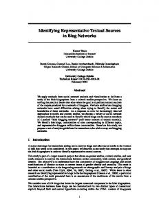
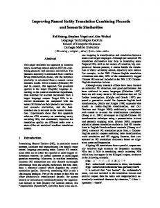
heuristics described in Section 3. We then calculated the percentage improvement over of the six other heuristics. The results are summarized in Figures 1 and 2. Figure 1 depicts the average improvement of the six heuristics over with respect to parallelism, where the graphs are sorted into 11 bins with parallelism values: [0 ? 2], [2 ? 4] : : :, [18 ? 20], [20+]. Figure 2 depicts the average improvement with respect to graph size. Data was again collected at 11 intervals, [0 ? 20]; : : :; [200+]. Due to space limitations, these gures show results for 2, 4, and 12-processor systems; however these are representative. is the premier performer for 2 and 4-processor systems, but is best for low levels of parallelism in a 12-processor system. HLFET
HLFET
ETF
HDLFET
Figure 1 reveals that in a 2-processor system, every heuristic has peak performance when the parallelism is approximately two. Similarly in 4-processor and 12-processor systems, Figure 1 shows that peak performance occurs when parallelism is slightly over 4 and 12 respectively. We explain the observation of this sensitivity to parallelism in three steps. (1) When the parallelism is smaller than the number of processors, there is little improvement over . (2) When the amount of parallelism is near the number of processors, peak performance improvements over are observed. This is because when the parallelism matches the number of processors, a carefully selected favailable processor, executable taskg pair, minimizing the e�ect of IPC delay, will result in a superior schedule. If high quality schedules are required it may be desirable to use or in this situation. (3) When the parallelism is greater than the number of processors, performance improvements drop. HLFET
HLFET
DLS
ETF
There is no indication from Figure 2 that graph size a�ects the performance of the heuristics. However, a large graph is better scheduled on a large number of processors, while a small graph is better scheduled on a small number of processors. This might be caused by the parallelism variations.
4.2 Performance of , DS
MIPCF
and
LIPF
Figure 1 yields an interesting observation about the relationship between and . Generally, complements when the parallelism changes. When the number of executable nodes is greater than the number of available processors, may prevent scheduling a high level node with heavy IPC cost. Thus has better performance when the parallelism is greater than the number of processors. However, when the number of executable nodes is smaller than the HLFET/SN
HDLFET/SP
HDLFET/SP
HLFET/SN
HDLFET/SP
HDLFET/SP
10
|
32
|
28
|
24
|
20
|
16
|
12
|
8
|
4
|
% Improvement over HLFET
36
HDLFET/SP
DS
HDLFET
DLS
ETF
|
0 |
HLFET/SN
02
20 0+ 2
20 0+ 2
20 0+ 2
20 0+ 2
20 0+ 2
20 +
Parallelism
32
|
28
|
24
|
20
|
16
|
12
|
8
|
4
|
% Improvement over HLFET
Processors = 12
HLFET/SN
DS
HDLFET
DLS
ETF
|
0 |
HDLFET/SP
02
20 0+ 2
20 0+ 2
20 0+ 2
20 0+ 2
20 0+ 2
20 +
Parallelism
32
|
28
|
24
|
20
|
16
|
12
|
8
|
4
|
% Improvement over HLFET
Processors = 4
HLFET/SN
DS
HDLFET
DLS
ETF
|
0 |
HDLFET/SP
02
20 0+ 2
20 0+ 2
20 0+ 2
20 0+ 2
20 0+ 2
20 +
Parallelism Processors = 2
Figure 1: Relative Performance of 6 Heuristics to HLFET for Di�erent Parallelism 11
|
28
|
24
|
20
|
16
|
12
|
8
|
4
|
% Improvement over HLFET
32
HLFET/SN
DS
HDLFET
DLS
ETF
|
0 |
HDLFET/SP
020
200 0+ 20
200 0+ 20
200 0+ 20
200 0+ 20
200 0+ 20
200 +
Graph Size (Number of Nodes)
32
|
28
|
24
|
20
|
16
|
12
|
8
|
4
|
% Improvement over HLFET
Processors = 12
HLFET/SN
DS
HDLFET
DLS
ETF
|
0 |
HDLFET/SP
020
200 0+ 20
200 0+ 20
200 0+ 20
200 0+ 20
200 0+ 20
200 +
Graph Size (Number of Nodes)
32
|
28
|
24
|
20
|
16
|
12
|
8
|
4
|
% Improvement over HLFET
Processors = 4
HLFET/SN
DS
HDLFET
DLS
ETF
|
0 |
HDLFET/SP
020
200 0+ 20
200 0+ 20
200 0+ 20
200 0+ 20
200 0+ 20
200 +
Graph Size (Number of Nodes) Processors = 2
Figure 2: Performance of 6 Heuristics Relative to HLFET for Di�erent Graph Sizes 12
number of processors, can prevent choosing an unsuitable processor requiring a large data transfer in order to process the node. Therefore has better performance when the parallelism is smaller than the number of processors. HLFET/SN
HLFET/SN
Our heuristic, , was derived from these insights. Recall that in , if the number of available processors is greater than of the executable nodes, is used while is used otherwise. The performance of is not just the maximum of and : at the beginning of each scheduling step, makes a ner decision by comparing the number of available processors and the number of executable nodes. DS
DS
HLFET/SN
HDLFET/SP HLFET/SN
DS
HDLFET/SP
DS
Figure 1 indicates the success of . Its performance is almost always better than either or . In a 12-processor system, it even performs better than and for low levels of parallelism. For 2 and 4-processor systems, is comparable to , while for a 12-processor system, has better peak performance. Still, in no case is ' performance substantially worse than any other heuristic. Finally, as will be shown in Section 5, the compile time for is dramatically lower than for either or , and signi cantly better than . DS
HLFET/SN
DLS
HDLFET/SP
ETF
DS
HDLFET
HDLFET
DS
DS
DLS
Heuristic HLFET/SN HDLFET/SP DS HDLFET DLS ETF
0-2 -0.1 0.6 .07 0.1 .01 .08
ETF
HDLFET
Table 2: E�ectiveness of MISF (%) Parallelism 2-4 4-6 6-8 8-10 10-12 12-14 14-16 -0.9 1.8 -0.9 0.5 0.7 0.2 -1.3 2.4 0.6 -.05 0.8 .09 0.7 1.3 0.6 0.1 0.3 1.3 .09 0.7 -1.3 0.8 0.8 -.04 1.1 .09 0.7 -1.3 0.5 .05 0.3 0.2 0.1 0.2 0.3 0.1 -0.4 0.2 0.4 -0.1 0.2 0.2
16-18 0.2 0.4 -0.3 0.4 0.1 0.3
18-20 0.3 0.1 0.2 1.2 0.3 0.1
20+ 0.1 .01 0.2 0.3 0.2 0.1
As previously described our other two techniques are \add-on's" to existing heuristics, in the manner of . To determine the e�ectiveness of itself, we took the six heuristics discussed in the previous Subsection and ran several tests using as a tie-breaker. The percentage improvement results in Table 2 for a 4-processor system are representative. As can be seen, provided negligible improvement. MISF
MISF
MISF
MISF
We suspected that the reason for 's poor showing was the fact that it ignores IPC costs. As a result we developed and implemented, which breaks a tie by selecting the task with highest IPC cost. To test the e�ectiveness of , we constructed two priority lists for a LGDFG. One was obtained from task levels, the other by placing tasks in descending order of their task levels and the IPC cost. For the sake of simplicity, we present results from applying to the two priority lists. The e�ectiveness of MISF
MIPCF
MIPCF
HDLFET
13
|
28
|
24
|
20
|
16
|
12
|
8
|
4
|
% Improvement over HLFET
32
|
0|
HDLFET HDLFET-MIPCF
02
20 +
Parallelism
Figure 3: Performance of HDLFET and HDLFET-MIPCF Relative to HLFET can be measured by the di�erences in makespans. Figure 3 shows that improved upon by only about 2 percent. However may still be worth employing as it incurs little overhead since the priority list is constructed before the list scheduling begins. MIPCF
MIPCF
HDLFET
MIPCF
Since neither nor performed terribly well, we took a slightly di�erent approach for our nal technique. As discussed in Section 3, is a mechanism to assign priorities to available processors. MISF
MIPCF
LIPF
To investigate the e�ectiveness of , the performance of , , , , and were compared. We tried each with 350 random LGDFGs in an 8-processor system. Figure 4 shows that the performance of with is close to . That is, there is a 5 to 10 percent improvement when is used! LIPF
HDLFET/SP-LIPF
DS
DS
LIPF
DS-LIPF
HDLFET/SP
HDLFET
HDLFET
LIPF
Furthermore does not incur overhead. If the available processor list is arranged in ascending order of processor index (as is done in the other existing heuristics), the list has to be resorted when a processor is added or removed from the available processor list. However, under the newly available processor is always placed on the top of the available processor list. Adding or removing a processor to the top of the list does not require resorting it. Since not only improves scheduling performance, but also saves the computation time of sorting the available processor list, we recommend its use in all list scheduling heuristics. LIPF
LIPF
LIPF
14
|
35
|
30
|
25
|
20
|
15
|
10
|
5
|
% Improvement over HLFET
40
DS, DS-LIPF
HDLFET
With LIPF Base Heuristic
|
0|
HDLFET/SP, HDLFET/SP-LIPF
02
20 +
02
20 +
02
20 +
Parallelism Effectiveness of LIPF
Figure 4: Performance of Heuristics with and without LIPF Relative to HLFET
5 A Comparison of Compile Time E�ciency In this section, the compile time e�ciency of the seven basic heuristics is compared. When the sizes of precedence graphs vary, the total compile time consumed by a list scheduling heuristic varies greatly due to the graph sizes. The compile time consumption also depends on the number of processors. In order to make the compile time e�ciency comparison results easy to interpret, we collect normalized compile times. The normalized compile time is de ned as the compile time per node per processor (CTNP), or Time (5) CTNP = Compile n�m In order to make the measurement more robust, the CTNP for each heuristic was averaged over 200 randomly generated precedence graphs. The simulation was run on a Sun SPARC 10 workstation, and the precedence graphs were scheduled onto 4 processors. As indicated in Section 4, has a stable performance close to the best list scheduling heuristics in our study. However, as shown in Figure 5, has much lower compile times than best performing heuristics| , and . In short, represents a good compromise between scheduling performance and compile time. DS
DS
HDLFET DLS
ETF
DS
6 Related Work We have already made a comprehensive survey of di�erent list scheduling heuristics and their performance, and we will not repeat that here. Instead, we brie y comment on the 15
DLS
SN = HLFET/SN
4000
|
3000
|
SP = HDLFET/SP
5000
|
Microseconds
|
6000
|
7000
ETF
HDLFET HLFET SN
DS
SP
|
1000
|
2000
|
0|
Heuristics
Figure 5: Compile Time E�ciency of the 7 Basic Heuristics two previous comparative studies, [1] and [11], most relevant to our work. In [1] and [11], list scheduling comparisons are made without accounting for IPC delay. In addition, there are three other factors that distinguish this work from [1] and [11]. 1. The Size of the Randomly Generated Graphs: [11] studied graphs with 5, 10, 20 and 30 nodes. In this study, we used much larger and more realistically sized graphs with more than 200 nodes. Testing with a large number of nodes is necessary to avoid possible biased comparisons. 2. The Number of Processors: [11] used � 3 processors. We found interesting results by testing the heuristics with a larger number of processors, in particular, peak performance improvement was achieved when the available parallelism was near the number of processors. 3. The Scale of Simulations: The comparative results in [1] were based on a small number of randomly generated precedence graphs. We observed a large variance in the relative performance of the heuristics on di�erent graphs, and found that a large number of samples was required to insure a stable mean.
7 Summary We compared a large number of proposed list scheduling heuristics for DSP multiprocessors with non-zero IPC delay. We found that no one heuristic consistently produces the 16
best schedules under all possible program structures and DSP multiprocessor con gurations. Our proposed heuristic has a very fast compile time, but still performs almost as well as much more complicated heuristics. It achieves this by intelligently combining other simpler heuristics. performance is better still when combined with our enhancement technique. is capable of improving the performance of most of the other basic heuristics as well. All heuristics studied achieved their peak performance when the amount of parallelism was roughly equal to the number of processors. DS
DS'
LIPF
LIPF
The comparison results reported in this paper are based on crossbar-switch connected DSP multiprocessors. It was assumed that each processor has one dedicated communication channel. Our future research will focus on DSP multiprocessor scheduling under more elaborate multiprocessor architecture constraints. We plan to investigate the e�ect of 1. Interconnection topologies such as mesh and bus connected multiprocessors; 2. Message routing techniques such as store-and-forward and virtual cut-through; 3. Multistage interconnection networks; 4. Processor resources such as the number of communication channels and dedicated communication hardware; 5. Heterogeneous DSP multiprocessor systems.
8 Acknowledgement Many people have contributed to this research. Stefan Roemer from Aachen University of Technology of Germany contributed to the design of a random graph generator during his visit in McGill as a visiting student. Palash Desai helped with a method to measure the CPU time in the compile time complexity study, and read the rst draft of the paper. Discussions with Dr. G. Ramaswamy was helpful to the design of the compile time complexity comparison experiment. The authors would like to thank Prof. Edward Lee for his suggestions in this comparative study. Finally, the authors are indebted to Dr. Gilbert Sih for his help and advice during this research. This work is supported by MICRONET. 17
References [1] T. L. Adam, K. M. Chandy, and J. R. Dickson. A comparison of list schedules for parallel processing systems. Communications of the ACM, 17(12):685{690, December 1974. [2] E. G. Co�man. Computer and Job-Shop Scheduling Theory. John Wiley & Sons, Inc., New York, New York, 1976. [3] Hesham El-Rewini and T. G. Lewis. Scheduling parallel program tasks onto arbitrary target machines. Journal of Parallel and Distributed Computing, 9(2):138{153, June 1990. [4] Michael R. Garey and David S. Johnson. Computers and Intractability: A Guide to the Theory of NP-Completeness. W. H. Freemann and Co., New York, New York, 1979. [5] R. L. Graham. Bounds on multiprocessing timing anomalies. SIAM Journal on Applied Mathematics, 17(2):416{429, March 1969. [6] P. D. Hoang. Compiling real-time digital signal processing applications onto multiprocessor systems. Memorandum No. UCB/ERL M92/68, Electronics Research Laboratory, University of California at Berkeley, 1992. PhD thesis. [7] T. C. Hu. Parallel sequencing and assembly line problems. Operations Research, 9(6):841{848, November 1961. [8] J. J. Hwang, Y. C. Chow, and F. D. Anger. Scheduling precedence graphs in systems with inter-processor communication time. SIAM Journal on Computing, 18(2):244{ 257, April 1989. [9] Hironori Kasahara and Seinosuke Narita. Practical multiprocessor scheduling algorithms for e�cient parallel processing. IEEE Transactions on Computers, 33(11):1023{1029, November 1984. [10] S. J. Kim and J. C. Browne. A general approach to mapping of parallel computations upon multiprocessor architectures. In Proceedings of the 1988 International Conference on Parallel Processing, volume III, pages 1{8, St. Charles, Illinois, August 15{19, 1988. [11] Walter H. Kohler. A preliminary evaluation of the critical path method for scheduling tasks on multiprocessor systems. IEEE Transactions on Computers, 24(12):1235{ 1238, December 1975. [12] C. C. Price and M. A. Salama. Scheduling of precedence constrained tasks on multiprocessor. The Computer Journal, 33(3):219{229, March 1990. 18
[13] H. Printz. Automatic Mapping of Large Signal Processing Systems to a Parallel Machine. PhD thesis, Carnegie-Mellon University, 1991. Published as Memorandum CMU-CS-91-101, Department of Computer Science. [14] Vivek Sarkar. Partitioning and Scheduling Parallel Programs for Multiprocessors. Research Monographs in Parallel and Distributed Computing. Pitman, London and The MIT Press, Cambridge, Massachusetts, 1989. Revised version of the author's Ph.D. dissertation (Stanford University, April 1987). [15] G. C. Sih. Multiprocessor scheduling to account for interprocessor communication. Memorandum No. UCB/ERL M91/29, Electronics Research Laboratory, University of California at Berkeley, 1991. PhD thesis. [16] Gilbert C. Sih and Edward A. Lee. A compile-time scheduling heuristic for interconnection-constrained heterogeneous processor architectures. IEEE Transactions on Parallel and Distributed Systems, 4(2):175{187, February 1993. [17] Gilbert C. Sih and Edward A. Lee. Declustering: A new multiprocessor scheduling technique. IEEE Transactions on Parallel and Distributed Systems, 4(6):625{637, June 1993. [18] W. H. Yu. LU Decomposition on a Multiprocessing System with Communication Delay. PhD thesis, UC-Berkeley, 1984.
A Scheduling Testbed The Scheduling Testbed is a software tool constructed for the purpose of this study. The testbed consists of three parts, the random graph generator, the implemented list scheduling heuristics, and the performance analyzer. Equipped with a random graph generator, the testbed is used as a multiprocessor scheduling heuristic comparative study tool. With the implemented heuristics, the testbed also assists in parallel code generation. The performance analyzer is used interactively to assist the analysis of obtained schedules.
Random Graph Generator The characteristics of precedence graphs have a strong impact on the performance of scheduling heuristics; therefore, it is desirable to be able to customize the precedence graphs generated by the random graph generator. A random graph is generated from several starting nodes. There are four actions that make the graph grow from the starting nodes | the extension action, the diverge action, 19
the converge action, and the random connection action. At each iteration, one of these four actions is selected at random. The extension action selects an exit node at random, generates a number of successors, and connects them to the selected exit node in a linear array. The diverge action selects an exit node at random, and generates a number of immediate successors to the selected exit node. The number of successors in extension and diverge actions is obtained at runtime from their respective uniformly distributed random functions. The converge action selects a number of exit nodes at random, and generates one immediate successor to the selected exit nodes. The random connection action chooses two nodes at random, and connects them in a way to avoid forming a loop in the precedence graphs. The sizes and parallelisms of randomly generated precedence graphs can be customized in the random graph generator. The sizes of the precedence graphs are adjusted by the number of iterations. Other factors determine the graph sizes as well; for example, the mean of extension and the mean of diverge. The parallelisms are modi ed by the number of starting nodes and the mean of diverge. The weight of nodes and the data units passed across the arcs are chosen from their respective random functions when the nodes and arcs are generated.
Implemented List Scheduling Heuristics Seven list scheduling heuristics are implemented in the testbed. They are , and . Three performance enhancement techniques, , and are also implemented. HLFET,
HLFET/SN, HDLFET/SP, HDLFET, DLS, ETF MISF
MIPCF
DS
LIPF
Performance Analyzer The performance analyzer does post-scheduling data processing. It reports the makespan of the schedule and the average utilization of the multiprocessor system. It also generates the following charts to assist to interpreting the scheduling results: Processor Utilization Chart The processor utilization chart displays the percentage of processor busy time. It is used to study the processor load balance. Comparison Charts These charts depict the percentage improvements compared to of a number of heuristics. Two kinds of comparison charts are of interest: (1) with respect to graph size, and (2) with respect to graph parallelism. These were illustrated in Section 4. They are also used as a tool to nd out the best heuristic for a speci c precedence graph. HLFET
20