of structured multivariate Normal (SMVN) models. These models consider a response vector as following a multivariate normal distribution with a limited number ...
MCMC algorithms for structured multivariate normal models William Browne*, Suna Akkol†
1
and Harvey Goldstein*
*University of Bristol, †University of Yuzuncu Yil, Turkey Summary In this paper we look at the use of MCMC methods for the general class of structured multivariate Normal (SMVN) models. These models consider a response vector as following a multivariate normal distribution with a limited number of parameters representing the mean vector and variance matrix. We in particular look at how multilevel models can be represented in this framework and show that a simple random walk Metropolis algorithm for such models can be very quick and outperform MCMC algorithms for the equivalent model in the standard ‘random effects’ framework on some simple examples. We show however that this computational advantage only holds for very simple models. We discuss model comparison which is more natural in this framework. We finish with discussion of other models that fit naturally in the framework and link to other work on these models. Keywords: Multilevel Modelling, Markov chain Monte Carlo (MCMC), structured multivariate normal models, Metropolis Hastings
1
Introduction
Statistical models that take account of the structure of the data that is collected are increasingly widely used. Often this structure involves some clustering in the dataset where certain observations are collected from the same cluster and it is believed that such observations should be more similar than observations collected from different clusters. The term ‘multilevel model’ is typically used to describe such models that deal with clustered data. There are (at least) two ways of describing a model for data with such clustering and we illustrate this here for a general normal response linear model with response vector y, predictor variables X and data collected on J clusters with nj observations in the jth cluster. 1 We
are grateful to (a) the ESRC for financial support for the first author, and (b) TUBITAK-BIDEB for financial support for the second author’s visit to the UK.
2
Firstly random effect (latent variable) models describe this structure by adding random (unobserved) effects, uj to a standard linear model so that we have the following: yij = Xij β + uj + eij uj ∼ N (0, σu2 ), eij ∼ N (0, σe2 ), i = 1, . . . , nj , j = 1, . . . , J
(1)
Here i indexes the observations in cluster j and so yij is the ith response on the j cluster, β is the fixed effect vector associated with the predictors X and uj are the random effects, one for each cluster. This model formulation is known as a random intercept or variance components model as the uj create differing intercepts for each cluster and is the standard one (with the addition of priors for β, σu2 and σe2 ) used with MCMC estimation. Assuming conjugate priors are used then this model can be fitted using a four step Gibbs sampling algorithm (see Browne (2003) for details of an implementation in MLwiN). Note that additional random effects that account for cluster specific effects of predictor coefficients (random slopes) can also be included in a multilevel model. The other formulation is to consider the whole response vector y following a multivariate Normal distribution as follows: y ∼ M V N (Xβ, V ) The clustering is now accounted for by the form given to V . We will describe such a model formulation as a structured multivariate normal (SMVN) model. In fact a simple linear model can also be described in this framework by letting V = σe2 I and in the random intercepts case given by (1) we can write yj ∼ M V N (Xj β, Vj ) Vj = σe2 Inj + σu2 Jnj
(2)
where yj is the response vector for the jth cluster, Xj is the matrix of p predictor variables for the jth cluster, Inj is the nj × nj identity matrix and Jnj is an nj × nj matrix of 1s. This formulation is the basis of the IGLS algorithm (Goldstein, 1986) that is used in the software package MLwiN (Rasbash et al. 2000). It is a straightforward exercise to verify that (1) does indeed imply (2). In this paper we consider using MCMC methods for this second formulation of the model and highlight some advantages and disadvantages. In particular we shall focus on the speed advantages from the use of this formulation. As computer processing speeds and memory continue, apparently, to obey Moore’s law, namely a power doubling approcimately every 2 years, it is sometimes argued that searching for more efficient computing algorithms should have a low priority since the performance of the hardware can be expected to achieve the same or superior effect within a reasonable time scale. While this may be true for certain applications, our own experience in the
3
social and medical sciences is that, as processing capacity improves, so does the ambition of the data analyst. One might even argue that Moore’s law should also be applied to the size of problems that data analysts are prepared to contemplate. This is particularly relevant to the use of very large administrative datasets from, for example health and education. These datasets are now available for analysis and will often include several million individual subjects with repeated observations and many variables, with various levels of clustering, so that processing time is crucial to the feasibility of completing an analysis within a realistic time scale. We would suggest, therefore, that the search for more efficient software algorithms is a worthwhile activity, and the practical justification for the topic of the present paper. In the next section we describe their use in the simple family of random intercept models. In section 3 we look at choosing between models and in particular testing whether clustering is important. In section 4 we look at random slopes models and see that adding extra random terms often removes the speed advantage of the framework. In section 5 we look at other models that naturally fit into this framework before finishing with some discussion.
2
Random intercept models
Multilevel models are used to account for underlying structure (clustering) in the data which are used in an analysis. The simplest form of multilevel model is the random intercept model (1) where a single random term is used for each cluster to account for within cluster similarity. There are many motivations for fitting a multilevel model. Generally we assume that the main focus in the analysis is the relationship between the response variable y and the predictor variables X. Then the structure of the data might be perceived as a nuisance that has to be accounted for in some way. This is the motivation behind techniques such as generalised estimating equations (GEE, Diggle, 1994) and the use of sandwich estimators (White, 1980) that adjust fixed effect standard errors to account for the clustering. Alternatively the structure of the data itself might be important and we might like to make inferences about the structure through the magnitude of the cluster level variance σu2 or the individual random effects uj . For example the between cluster variance (along with the level 1 variance) can be used to construct the variance partitioning coefficient (VPC) which estimates the importance of the clustering in the data for a particular observation and for a random intercept model is V PC =
σu2
σu2 + σe2
Note for the random intercept model the VPC does not depend on the value of the predictors and is identical to the intra-class correlation (ICC). It can be debated whether inferences about individual random effects should be
4
made. If the particular units that the random effects represent are themselves important then their exchangability might be questioned and they could instead be fitted as fixed effects. If however exchangability is not an issue and we have few observations on a particular cluster then a random effects model will shrink the corresponding cluster effect towards zero and prevent overconfidence in the effects associated with small clusters. Furthermore, as we shall see when we look at random coefficient models, fitting a fixed effect for every (potentially random) coefficient for every cluster becomes unwieldy when there is a large number of clusters and the random effects model which assumes a distribution for these coefficients is an efficient modelling procedure. The estimation of random effects to assess goodness of fit of the model assumptions, for example normality in (1), and to look for outliers is also appropriate. A disadvantage of the alternative SMVN formulation is that it doesn’t contain the random effects uj and so no goodness of fit testing of this type can be done. It is however possible (see Goldstein 2003 Appendix 2.2) to construct residuals conditional on the parameter estimates obtained from a model fitted using SMVN. The other disadvantage of the SMVN formulation is that the Bayesian random effects formulation (with conjugate priors) results in conditional conjugacy for all parameters and hence the use of a simple Gibbs sampling algorithm, whilst this is not true for the SMVN formulation. The two formulations will result in equivalent estimates assuming the same priors are used for β, σu2 and σe2 . It should be noted that in the SMVN formulation the parameter σu2 is really a covariance in the model and not a variance and therefore it can feasibly take negative values which can be interpreted as greater variability within clusters than in the population in general. A good example of this is litter effects in animal populations where competition for resources may generate more variability of weight or size in a litter than in a random sample from the population generally. In the SMVN formulation therefore, a negative value for this parameter presents no problems, and we can choose a prior that allows such negative values and this could be useful for model selection as we discuss later. We will here consider the SMVN model in a Bayesian framework and devise a random walk Metropolis algorithm for fitting the models. It should be noted that the fixed effects β will have a Gaussian full conditional distribution (Chib and Carlin, 1999) and so could alternatively be updated using Gibbs sampling but here we consider an algorithm with random-walk Metropolis steps for all parameters.
2.1
Constructing a random walk Metropolis algorithm
For Bayesian SMVN models we have 3 sets of unknown parameters, the fixed effects β, the level 2 random variance terms Ωu , which for the random intercept model consist of a single variance σu2 , and the level 1 variance σe2 .
5
All these parameters require prior distributions and so for generality we will assume generic priors p(β), p(σu2 ) and p(σe2 ). These then need to be combined with the likelihood to form the posterior distribution. The likelihood is as follows: L(y | β, σu2 , σe2 ) =
QJ
−nj /2 |Vj |exp j=1 (2π) where Vj = σe2 Inj
� − 12 (yj − Xj β)T Vj−1 (yj − Xj β) + σu2 Jnj .
�
As illustrated in McCulloch and Searle (2001) for special cases this likelihood can be simplified, for example, for the variance components model (a random intercept model with only a constant (β0 ) in the fixed effects) we have P log(L(y | β, σu2 , σe2 )) = − 21 N log 2π − 12 j log(σe2 + nj σu2 ) − 21 (N − J) log(σe2 ) 2 P yj −β0 )2 σ 2 P n (¯ − 2σ1 2 i,j (yij − β0 )2 + 2σu2 j σj 2 +nj σ2 e
P
where N = j nj and y¯j = model this becomes
e
P
i
e
u
yij /nj . For a general random intercept
P log(L(y | β, σu2 , σe2 )) = − 12 N log 2π − 12 j log(σe2 + nj σu2 ) − 21 (N − J) log(σe2 ) P P σ 2 P ( i (yij −Xij β))2 . − 2σ1 2 i,j (yij − Xij β)2 + 2σu2 j σ 2 +nj σ 2 e
e
e
u
Given the above we can choose starting values for all the parameters in the model and then construct a three step Metropolis Hastings algorithm.
Step 1 - Update the fixed effects β using univariate random walk Metropolis at iteration t + 1 as follows, for j = 1, . . . , p and with β(−j) signifying the β vector without component j: h i p(β (∗)|y,σ 2 ,σ 2 ,β(−j) ) βj (t + 1) = βj (∗) with probability min 1, p(βjj (t)|y,σ2u,σ2e,β(−j) ) u e = βj (t) otherwise, where βj (∗) ∼ N (βj (t), s2βj ) and p(βj | y, σu2 , σe2 , β(−j) ) ∝ L(y | β, σu2 , σe2 )p(βj ). Step 2 - Update σu2 using univariate random walk Metropolis at iteration t+1 as follows : i h p(σ 2 (∗)|y,β,σ 2 ) σu2 (t + 1) = σu2 (∗) with probability min 1, p(σu2 (t)|y,β,σ2e) u e = σu2 (t) otherwise, where σu2 (∗) ∼ N (σu2 (t), s2pu ) and p(σu2 | y, β, σe2 ) ∝ L(y | β, σu2 , σe2 )p(σu2 ).
6
Here as described previously in Browne (2006) we use a normal proposal distribution and assume that inadmissible values for σu2 will have zero likelihood or a prior of zero. The alternative is to use a truncated Normal proposal (and calculate the resulting Hastings ratio for each iteration) where the truncation point is zero for priors that force σu2 to be positive and −σe2 / maxj (nj ) otherwise. Step 3 - Update σe2 using univariate random walk Metropolis at iteration t+1 as follows : h i p(σ 2 (∗)|y,β,σ 2 ) σe2 (t + 1) = σe2 (∗) with probability min 1, p(σe2 (t)|y,β,σ2u) e u = σe2 (t) otherwise, where σe2 (∗) ∼ N (σe2 (t), s2pe ) and p(σe2 | y, β, σu2 ) ∝ L(y | β, σu2 , σe2 )p(σe2 ). Again we have the alternative here of a truncated normal proposal distribution with truncation point 0. To choose the values of the proposal standard deviations, sβj , spu and spe we use an adapting procedure due to Browne and Draper (2000) that consists of an additional adaptation period prior to burning in, in which the proposal distributions are tuned to give acceptance rates of roughly 50%.
2.2
Efficient Likelihood Evaluation
It is easier to work with the log-likelihood than the likelihood and for the general variance components model we have P log(L(y | β, σu2 , σe2 )) = − 12 N log 2π − 12 j log(σe2 + nj σu2 ) − 21 (N − J) log(σe2 ) P P σ 2 P ( i (yij −Xij β))2 . − 2σ1 2 i,j (yij − Xij β)2 + 2σu2 j σ 2 +nj σ 2 e
e
e
u
Here the majority of the computation lies in the last two terms with their summations of squared terms over the length of the dataset. We can speed up evaluation by considering summary statistics of the data that are constant through iterations. If we write y for the vector of responses yij and X forPthe matrix of predictor variables then we can write the penultimate term, i,j (yij − Xij β)2 = y T y − 2y t Xβ + β T X T Xβ. Now storing the sums of squares and cross product objects y T y, y T X and X T X results in far fewer numerical operations. By a similar argument the same objects can be constructed for each cluster and the operations for the inner i summation in the final term can be reduced. These speed ups rely on the fact that the number of observations in the dataset N (and the size of each cluster nj ) is far greater than the number of fixed effects p which is true in many cases.
7
2.3
Comparison of results for an example from education
We here consider a dataset of student exam scores (Rasbash et al. 2004) taken by students at age 16. We begin by fitting a variance components model and we have 4059 students in 65 schools. We compare the results and the MCMC chains from the above algorithm and the standard Gibbs sampling algorithm in MLwiN. For comparison of the chains we use the effective sample size (ESS) statistic described in Kass et al. (1998) which for each chain gives the size of an equivalent independent sample from the posterior distribution. For this example we use improper uniform priors for β, σu2 and σe2 although similar conclusions can be obtained with other ‘diffuse’ priors and we run for 100k iterations after a burnin of 5,000. The results can be seen in table 1. Table 1: Estimates and effective sample sizes for the variance components model MLwiN SMVN formulation Parameter Estimate (S.D.) ESS Estimate (S.D.) ESS β0 -0.012 (0.056) 4k -0.013 (0.056) 24k 0.184 (0.038) 65k 0.185 (0.038) 21k σu2 0.849 (0.019) 97k 0.849 (0.019) 25k σe2 Time 50s 2s We can see that although the SMVN formulation has worse ESS for the two variance parameters it is far quicker and wins on the metric ESS/s. It should be noted that we are using the standard MCMC algorithm in MLwiN which is not using hierarchical centering (Gelfand et al. 1995) which will increase the ESS for β0 . This is possible in the WinBUGS software package and the resulting ESS is 82k although the algorithm in WinBUGS took 250s.
3
Model comparison
The education dataset has a predictor variable, LRT which is a reading test that the students took at age 11. We can include this parameter in our model and fit a random intercept model using either of the formulations. The results are given in table 2 Here as with the variance components model we see generally smaller ESS for the SMVN formulation but a far faster algorithm means that the SMVN formulation gives better ESS/s values. If we wish to choose between the two models there are many possibilities. Perhaps the simplest comparison tool is to look at the chain for the additional parameter β1 as the variance components model is simply the random intercept model with β1 constrained to zero. Using either formulation this
8
Table 2: Estimates and effective sample sizes for the random intercept model MLwiN SMVN formulation Parameter Estimate (S.D.) ESS Estimate (S.D.) ESS β0 - intercept 0.004 (0.042) 5k 0.002 (0.042) 25k β1 - LRT 0.563 (0.013) 83k 0.563 (0.012) 25k σu2 0.101 (0.021) 59k 0.101 (0.022) 20k σe2 0.566 (0.013) 97k 0.566 (0.013) 24k Time 57s 3s chain never crosses the zero value and so there is no support for the simpler model. A more complicated example is testing for the existence of a set of random effects or equivalently their variance, σu2 . The model without the random effects effectively has σu2 constrained to equal zero, however in the random effects formulation σu2 is truly a variance and so requires a prior that has all its mass on positive values and hence it’s posterior chain will never cross the zero value. An advantage of the SMVN approach is that a prior with mass on negative values can be used, as in this framework σu2 is really representing covariance within the larger variance matrix V (and perhaps should be relabelled σuu ). To illustrate this point we simulated 4059 fully independent standard normal responses and then match these responses to the data structure of the tutorial dataset. We then fitted a variance components model using each framework and got the following results: Table 3: Estimates and effective sample sizes for a simulated variance components model with zero level 2 variance MLwiN SMVN formulation Parameter Estimate (S.D.) ESS Estimate (S.D.) ESS β0 -0.001 (0.017) 72k -0.003 (0.016) 23k σu2 0.002 (0.002) 2.3k 0.000 (0.003) 18k σe2 1.022 (0.023) 99k 1.024 (0.023) 24k Time 50s 2s Here we have similar estimates from the two approachs however the MLwiN estimate is based upon a chain that never goes negative whilst the SMVN formulation chain can be seen in figure 1. We see here that the posterior has considerable mass below zero and so we can use a 95% credible interval to show that zero cannot be rejected as a potential estimate. Note that chapter 5 of Box and Tiao (1973) give a nice discussion of the problem of negative variance in random effect models which can result from a sampling theory approach.
100 50 0
Density
150
9
0.00
0.01
0.02
0.03
level 2 variance Figure 1: Kernel density plot of posterior of σu2 under the SMVN formulation
3.1
Deviance Information Criterion
The Deviance information criterion (DIC) was proposed by Spiegelhalter et al. (2002) as a method for comparing statistical models fitted using MCMC. Although the DIC has it’s critics, including several of the discussants of the original paper read at the RSS, it’s ease of calculation and the lack of implementation of alternatives has led to considerable use in applied articles. The DIC like other information criterions is a combination of the fit and complexity of a model. The fit in this case is the mean deviance and the complexity is twice the ‘effective’ number of parameters. One problem with the DIC is it’s lack of invariance to the ‘focus’ of the model, so for example a reparameterisation of a model and calculation of the DIC using this new parameterisation may result in different numerical estimates. One nice feature of the use of the DIC with the SMVN formulation described in this paper is that due to the lack of random effects, the ‘effective’ number of parameters is (usually) close to the actual number of parameters
10
in the model. Table 4 gives DIC values for the two models considered earlier along with the random slopes model in the next section based on the SMVN method. Table 4: DIC Estimates for three models using the SMVN formulation ¯ ¯ Model D(θ) D(θ) pD DIC Model 1: Variance Components 11013.8 11010.9 2.9 11016.7 Model 2: Random Intercepts 9361.4 9357.5 3.9 9365.3 Model 3: Random Slopes 9323.5 9321.2 2.3 9325.7 Here we see that the models give successively smaller DIC values suggesting better models. The introduction of the LRT predictor (moving from models 1 to 2) and the introduction of random slopes (moving from models 2 to 3) both result in lower DIC values. The effective number of parameters pD is approximately equal to the actual number of parameters in the first two model but is lower in the random slopes model. This gives some evidence that the DIC in this framework might be easier to understand and actually will be equivalent to the AIC.
4
Random slopes models
A natural extension of the variance components and random intercepts model is the random slopes model where we allow predictor variables to have different effects for each higher level unit. In the education example we can consider allowing the effect of the predictor LRT to vary across schools. In the random effects framework we would write this as yij = β0 + LRTij β1 + u0j + LRTij u1j + eij uj ∼ M V N (0, Ωu ), eij ∼ N (0, σe2 ), i = 1, . . . , nj , j = 1, . . . , J
(3)
where uj = (u0j , u1j )T . In the SMVN framework we can write a random slopes model as yj ∼ M V N (Xj β, Vj ) Vj = σe2 Inj + Xj Ωu XjT
(4)
where Xj = (X1j , . . . , Xnj j )T and Xij = (1, LRTij ) in our example. This is similar to (2) but with the within group variance matrices Vj depending on the predictor variable LRT . We then have the general MVN likelihood function for each block and the likelihood is as follows:
L(y | β, Ωu , σe2 ) =
J Y
� � 1 (2π)−nj /2 |Vj |exp − (yj − Xj β)T Vj−1 (yj − Xj β) . 2 j=1
11
We adapt the random walk Metropolis algorithm described in section 2.1 to random slopes models. The steps (1) and (3) for the fixed effects and the level 1 variance are unchanged and so we adapt step (2) as follows: Step 2 - Update Ωu [i, j], i = 0, 1j ≤ i using univariate random walk Metropolis at iteration t + 1 as follows : i h p(Ω [i,j](∗)|y,β,σ 2 ) Ωu [i, j](t + 1) = Ωu [i, j](∗) with probability min 1, p(Ωuu [i,j](t)|y,β,σ2e) e = Ωu [i, j](t) otherwise, where Ωu [i, j](∗) ∼ N (Ωu [i, j](t), s2pu[i,j] ) and p(Ωu [i, j] | y, β, σe2 ) ∝ L(y | β, Ωu , σe2 )p(Ωu ). Note that spu[i,j] are the proposal standard deviations that will be adapted as before (Browne and Draper (2000)). Here as described previously in Browne (2006) we use a normal proposal distribution for each element of Ωu and assume that inadmissible sets of values for Ωu will have likelihood or prior zero. For the variance components model we were able to calculate a negative lower bound (−σe2 / maxj (nj )) for the parameter σu2 that resulted in positive definite matrices Vj and this allowed us to test if σu2 was significantly different from 0. For the random slopes model there is not an equivalent single lower bound since we now have several parameters in the matrix and hence the bound for each parameter will depend on the values of the rest of the matrix. Moreover, even if we did carry out such a check, this would not guarantee that any of the Vj matrices remained positive definite for all possible values of the predictor X and would raise interpretational difficulties. Instead, therefore, we shall treat the matrix Ωu as a true variance matrix (as in the random effects framework) by using a prior that only has support for positive definite matrices so that we can easily test that a proposed variance matrix is positive definite by using a Cholesky decomposition. Assuming that Ωu is strictly a variance matrix rather than a set of parameters that describe correlations in the variance matrix V does result in the lack of a nice model comparison test as used in section 3 for variance components models and so in further work we will investigate if we can calculate conditional bounds for each of the parameters in Ωu when assuming only that V is positive definite but not necessarily Ωu and also study interpretational issues. The alternative approach to using normal proposals is to use truncated Normal proposals (and calculate the resulting Hastings ratio for each iteration) where the truncation points are such that Ωu remains positive p we have Ωu [0, 0] > 0, Ωu [1, 1] > 0 p definite. In our 2 × 2 example and − Ωu [0, 0]Ωu [1, 1] < Ωu [0, 1] < Ωu [0, 0]Ωu [1, 1] but such constraints increase in number as the size of the variance matrix increases and the truncated normal method becomes impractical (see Browne (2006)).
12
4.1
Efficient Likelihood Evaluation
The likelihood function L(y | β, Ωu , σe2 ) has been simplified by considering the MVN vector as a set of independent MVN blocks corresponding to level 2 units whose likelihood can be evaluated separately. This however still leaves blocks of size of up to 198 in the education example. For these blocks we need to invert the variance matrices Vj every time we propose new values for any of the variance parameters in the model. Inverting these blocks directly is computationally prohibitive and the algorithm can potentially be incredibly slow. We can, however, use matrix algebra results to speed things up. We can use the following matrix identity given in Goldstein(1986): (A + BCB T )−1 = A−1 − A−1 BC(I + B T A−1 BC)−1 B T A−1 . In our example we then have 1 1 Vj−1 = 2 Inj − 2 Xj Ωu σe σe
XjT Xj I2 + Ωu σe2
!−1
XjT .
This will remove the need to invert matrices of upto size 198 × 198 and instead we will have matrices of size 2×2 to invert allbeit with some additional matrix multiplications. We will now look at using this algorithm on a random slopes model for the education dataset. Table 5 gives results for fitting a random slopes regression model to the tutorial dataset with a burnin of 5,000 iterations and a run of 100,000 iterations. Table 5: Estimates and effective sample sizes for the RSR model MLwiN SMVN formulation Parameter Estimate (S.D.) ESS Estimate (S.D.) ESS β0 - intercept -0.011 (0.042) 4.3k -0.012 (0.043) 19k β1 - LRT 0.556 (0.021) 15k 0.556 (0.021) 18k Ωu [0, 0] 0.103 (0.022) 58k 0.103 (0.022) 11k Ωu [0, 1] 0.020 (0.008) 36k 0.020 (0.008) 9k Ωu [1, 1] 0.018 (0.006) 22k 0.018 (0.006) 11k σe2 0.554 (0.013) 93k 0.554 (0.013) 24k Time 96s 3hrs Here we see good agreement between the two formulations and not much to choose in terms of ESS however even with our efficient likelihood evaluations the fact that the SMVN formulation takes over 100 times longer means it is clearly for this example not a practical competitor. Before we dismiss the SMVN formulation as being totally unsuitable for random slopes model
13
we will consider another example and application of random effect models, namely repeated measures models.
4.2
A balanced repeated measures model
The education dataset has some large clusters of observations and is unbalanced both in terms of cluster size and predictor values. We will here consider a smaller example on the weights of laboratory rats studied in Gelfand et al. (1990). This dataset consists of the weights of 30 rats that were measured weekly for 5 weeks. We will consider the following random slopes model: yij = β0 + agei β1 + u0j + agei u1j + eij uj ∼ M V N (0, Ωu ), eij ∼ N (0, σe2 ), i = 1, . . . , nj , j = 1, . . . , J
(5)
where uj = (u0j , u1j )T , i indexes time points and j indexes rats. In the SMVN framework we can write the model as yj ∼ M V N (Xj β, Vj ) Vj = σe2 Inj + Xj Ωu XjT
(6)
but as all rats are the same age at each measurement then we have Xj = Xj′ ∀j, j ′ and hence we can replace Vj with V1 ∀j. This will reduce the computation as rather than evaluating 30 separate Vj−1 we can evaluate one and use it for each rat. In table 6 we give estimates from the random effects and SMVN formulations of the model. Table 6: Estimates and effective sample sizes for the rats model MLwiN SMVN formulation Parameter Estimate (S.D.) ESS Estimate (S.D.) ESS β0 - intercept 106.65 (2.584) 6.5k 106.59 (2.598) 18k 6.188 (0.119) 3.6k 6.186 (0.119) 18k β1 - age Ωu [0, 0] 154.73 (61.74) 36k 156.43 (63.46) 7.6k Ωu [0, 1] -1.440 (2.099) 33k -1.474 (2.114) 6.9k Ωu [1, 1] 0.344 (0.131) 41k 0.344 (0.129) 7.9k σe2 37.91 (5.856) 97k 37.83 (5.857) 20k Time 20s 7s Here we see again that both formulations give similar estimates and have reasonably similar overall performance in terms of ESS, with the random effects framework giving better ESS for random parameters but worse for fixed effects. The SMVN formulation is competitive in terms of computation time and is actually quicker than the standard formulation. This is in part due to the speed up due to the balanced data and without the speed up the method took 86 seconds. This does however only represent a factor of
14
4 rather than 100 between the two methods for the rats dataset and this is because the largest block is of size 5 (as opposed to 198) and the number of multiplications involved in the evaluation of the likelihood is O(n2j ). This leads us to conclude that the SMVN formulation may not be so bad for random slopes models as long as the block sizes aren’t too big but also that the speed up due to the balanced structure might not be so impressive for longer repeated measures series.
5
Other structured multivariate normal models
The number of models that can be written in the general multivariate normal y ∼ M V N (Xβ, V ) is vast. We have here concentrated on two level models that are generally considered in a random effects framework when using MCMC. One feature of these models is their block structure and the fact that we can write the model as: yj ∼ M V N (Xj β, Vj ) for some blocks j = 1, ..., J. This means that the computationally intensive part of the likelihood evaluation (inverting the matrix V ) is replaced by the computationally quicker inversion of the variance matrices for the individual blocks Vj . This suggests that other models that might be suitable for MCMC fitting via the structural MVN formulation would have different structural forms for the matrics Vj while maintaining between block independence. Examples of such models that have been fitted (in a maximum likelihood setting) by extending the IGLS algorithm are multilevel time series models (Goldstein et al. 1994). Here the correlation between observations within a cluster depends on the time gap between the two observations. Browne (2006) describes an MCMC algorithm for the rats repeated measure data that assumes an autoregressive (AR(1)) structure for the time gaps. As the time gaps are all equal this results in the following correlation matrix with ρ estimated at 0.94 : 1 ρ ρ2 ρ3 ρ4 ρ ρ ρ2 ρ3 2 1 ρ ρ2 D= . ρ3 ρ2 1 ρ ρ ρ 1 ρ ρ4 ρ3 ρ2 ρ 1 Browne (2006) then uses separate mean and variance parameters for each timepoint resulting in a model with 5 parameters to explain mean behaviour
15
and 6 parameters to explain the variance matrices Vj . The random slopes model described in section 4 uses only 2 parameters to explain mean and 4 parameters to explain the variance matrices Vj which results in a correlation between two observations at times s and t, ρs,t as
ρs,t = p
Ωu [0, 0] + (s + t)Ωu [0, 1] + stΩu [0, 1] (Ωu [0, 0] + 2sΩu [0, 1] + s2 Ωu [0, 1] + σe2 )(Ωu [0, 0] + 2tΩu [0, 1] + t2 Ωu [0, 1] + σe2 )
which will change both with the time gap between the measures and also the time of the measures. If we use the estimates we have for the random slopes model we get
D=
1 0.779 0.720 0.653 0.592
0.779 1 0.829 0.800 0.765
0.720 0.829 1 0.875 0.863
0.653 0.800 0.875 1 0.910
0.592 0.765 0.863 0.910 1
.
These correlations are smaller than those in the AR(1) model in Browne (2006) but this is in part due to the AR(1) model using more parameters to estimate the mean and variance structure than the random slopes model. It is possible to fit many other structures to the within block variance matrices. The balanced repeated measures situation with the same structure for the within block matrix for each block clearly will have the greatest computational speed advantages but the same models can be fitted to nonbalanced structures. When the model does not have within block variance matrices of the form (A + BCB T ), then we cannot use the result in section 4.1 which will result in slower execution. Between block correlations as might be present if there are spatial relationships between blocks of responses, for example distances between schools are probably best not considered in the SMVN formulation and instead a latent variable random effects framework is much better. We will consider between block correlations in future work.
6
Discussion
In this paper we have considered how structured MVN models might be implemented using MCMC estimation. We have in the main considered how multilevel models that are commonly fitted using a random effects formulation when using MCMC might be fitted in the structured MVN formulation. We have shown the advantage this presents in terms of model comparison and computational speed for simple examples. We have also shown how for more complex models with further random effects the computational speed
16
advantage disappears and the structured MVN framework can be impractical. We have briefly looked at other structured MVN models that fit the general framework. In practical implementations it should be possible to interrogate the data structure in order to estimate the relative efficiencies of the two different algorithms we have studied. In further work we will look at rapid methods for carrying out such calculations so that a software package can choose the most efficient procedure for any given specified model.
References Box, G.E.P. and Tiao, G.C. (1973). Bayesian Inference in Statistical Analysis. Reading, Mass., Addison-Wesley. Browne, W.J. (2003). MCMC Estimation in MLwiN. London: Institute of Education, University of London Browne, W.J. (2006). MCMC Algorithms for constrained variance matrices. Computational Statistics and Data Analysis 50: 1655-1677. Browne, W.J. and Draper D. (2000). Implementation and performance issues in Bayesian and likelihood fitting of multilevel models. Computational Statistics 15: 391-420. Chib, S and Carlin, B.P. (1999). On MCMC sampling in hierarchical longitudinal models. Statistics and Computing, 9, 17–26. Diggle, P.J., Liang, K-Y. and Zeger, S.L. (1994) Analysis of Longitudinal Data. Oxford, Clarendon Press. Gelfand, A.E., Hills, S.E., Racine-Poon, A. and Smith, A.F.M (1990). An illustration of Bayesian inference in normal data models using Gibbs Sampling. Journal of the American Statistical Association 85: 972-985 Gelfand, A.E., Sahu, S.K. and Carlin, B.P. (1995). Efficient parameterizations for normal linear mixed models. Biometrika 82, 479-488. Goldstein, H. (1986). Multilevel mixed linear model analysis using iterative generalised least squares. Biometrika 73, 43-56. Goldstein, H. (2003). Multilevel Statistical Models. (Third edition) London: Edward Arnold. Goldstein, H., Healy, M.J.R. and Rasbash, J. (1994). Multilevel Time Series Models with applications to repeated measures data. Statistics in Medicine 13: 1643-1655. Kass, R.E., Carlin, B.P., Gelman, A. and Neal, R. (1998). Markov chain Monte Carlo in practice: a roundtable discussion. American Statistician, 52, 93–100. McCulloch, C.E. and Searle, S.R. (2001). Generalized, Linear and Mixed Models. New York: John Wiley and Sons. Rasbash, J., Browne, W.J., Healy, M, Cameron, B and Charlton, C. (2000). The MLwiN software package version 1.10. London: Institute of Education, University of London. Rasbash, J., Steele, F., Browne, W.J. and Prosser, B. (2004). A User’s Guide to MLwiN. London: Institute of Education, University of London.
17
Spiegelhalter, D.J., Best, N.G., Carlin, B.P. and van der Linde, A. (2002). Bayesian measures of model complexity and fit. Journal of the Royal Statistical Society, Series B 64: 583-640. White H (1980). A heteroscedasticity-consistent covariance matrix estimator and a direct test for heteroscedasticity. Econometrica, 48, 817-830.