MDP Algorithms for Portfolio Optimization Problems in pure Jump Markets Nicole B¨auerle ∗, Ulrich Rieder
†
Abstract We consider the problem of maximizing the expected utility of the terminal wealth of a portfolio in a continuous-time pure jump market with general utility function. This leads to an optimal control problem for Piecewise Deterministic Markov Processes. Using an embedding procedure we solve the problem by looking at a discrete-time contracting Markov Decision Process. Our aim is to show that this point of view has a number of advantages, in particular as far as computational aspects are concerned. We characterize the value function as the unique fixed point of the dynamic programming operator and prove the existence of optimal portfolios. Moreover, we show that value iteration as well as Howard’s policy improvement algorithm work. Finally we give error bounds when the utility function is approximated and when we discretize the state space. A numerical example is presented and our approach is compared to the approximating Markov chain method. AMS 2000 Subject Classification: Primary 91B28, 93E20 Secondary 90C39, 60G55 Keywords: Portfolio Optimization, Piecewise Deterministic Markov Processes, Markov Decision Process, Operator Fixed Points, Approximation Algorithms.
∗
Institut f¨ ur Stochastik, Universit¨ at Karlsruhe (TH), D-76128 Karlsruhe, Germany, email:
[email protected] † Institut f¨ ur Optimierung und Operations Research, Universit¨at Ulm, D-89069 Ulm, Germany, email:
[email protected]
1
Introduction
In this paper we consider the classical problem of maximizing the expected utility of the terminal wealth of a portfolio in a financial market. However, in contrast to most papers on this subject, we consider a continuous-time pure jump market. More precisely, we assume that jumps in the stock prices arrive according to a Poisson process and that the relative jump heights of the stocks are iid vectors. The behavior of the stock prices between jumps is purely deterministic. Thus, the price processes fall in the class of so-called Piecewise deterministic Markov processes (PDMP). It is well-known that the model parameters can be chosen such that this market model approximates a L´evy market arbitrarily well. We restrict our exposition to a fairly simple model but extensions are also discussed which do not complicate the analysis. Note that we do not assume a special form for the utility function. This model has various advantages over jump-diffusion markets, in particular as far as computational aspects are concerned. By considering the embedded jump process, the optimization problem can be formulated as a discrete-time Markov Decision Process (MDP). Our main aim is to show that this point of view implies a number of interesting results: (i) The first one is that the value function can be characterized as the fixed point of a dynamic programming operator. This operator can be shown to be contracting which establishes uniqueness of the fixed point. Differentiability of the value function is not needed. (ii) The existence of an optimal portfolio strategy is rather easy to prove. (iii) Established MDP algorithms like value iteration or Howard’s policy improvement algorithm can be used to solve the problem as an alternative to the solution of the Hamilton-Jacobi-Bellman equation. In our numerical example the implementation of the value iteration on a grid outperforms the result of the so-called approximating Markov chain method (see Kushner and Dupuis (2001)) which is a standard algorithm for solving stochastic control problems. (iv) Due to the contraction property of the operator, the convergence of numerical approximation schemes can be shown easily. The paper is organized as follows: In Section 2 we introduce the market model and the portfolio problem. This market model is nicely presented in Jacobsen (2006), however has been used before e.g. by Sch¨al (2005) and Kirch and Runggaldier (2005). A different pure jump market model can be found in Norberg (2003). In Section 3 we show how the optimization problem for the piecewise deterministic Markov process can be solved by a discrete-time Markov Decision Process. This method is rather standard and is e.g. explained in Davis (1993) or Almudevar (2001) for general PDMP. However in finance it has only been used by Kirch and Runggaldier (2005) for an efficient hedging problem with a very special stock price process. Section 4 uses the MDP formulation to show that the value function is the unique fixed point of a dynamic programming (DP) operator and that the value iteration as well as the policy iteration hold. Moreover, we prove the existence of an optimal stationary 1
portfolio strategy. Surprisingly, though the utility function is unbounded (in contrast to Kirch and Runggaldier (2005)) it is possible to introduce a certain weighted supremum norm on the function space such that the DP operator is contracting. This observation is crucial for most of the results which follow. We like to note here that, though existence results for MDPs are well-established (see e.g. Bertsekas and Shreve (1978)), it is rather profound to use the right topology on the action space in order to obtain the desired result. In this section also some model extensions are discussed like regime switching of model parameters and additional risk constraints. In Section 5 we present some computational methods and approximation procedures which arise from the MDP formulation and which are an interesting addition to the traditional HJB approach. More precisely, we show that Howard’s policy improvement algorithm is valid. Howard’s algorithm allows to find (if not run until termination which yields the optimal policy) a good policy after a reasonable number of steps. Then we use the properties of the DP operator to approximate the value function by approximating the utility function of the problem. In this case, also the optimal portfolio strategy is approximated. This complements results of Jouini and Napp (2004) who have investigated this question in diffusion markets. It turns out that the use of the DP operator simplifies the analysis considerably. Finally, we give an error bound on the distance to the true value function when we use the iterates of a DP operator which is concentrated on a grid of the state space only. A numerical example is presented in Section 6 and our approach is compared to the approximating Markov chain method.
2
The Model
We consider a special class of continuous-time financial markets where asset dynamics follow a so-called piecewise deterministic Markov process (PDMP). The reason is twofold: First it can be shown that general L´evy processes can be approximated arbitrarily close by such type of processes and second, optimization problems arising from these models can essentially be solved via the theory of discrete-time Markov Decision Processes (MDP). The financial market is as follows: Suppose T > 0 is the time horizon of our model and we have a probability space (Ω, F, P ) and on this space there is a homogeneous c`adl`ag Poisson process N = (Nt ) with constant rate λ > 0 and a sequence of independent and identically distributed random vectors (Yn ) with values in (−1, ∞)d . The Yn0 s are assumed to have a distribution Q and are itself independent of (Nt ). Thus, we can define the Rd -valued compound Poisson process Nt X Ct := Yn . n=1
Let us denote by (Ft ) the filtration generated by C = (Ct ). By (Ctk ) we denote the k-the component of this process. We suppose that we have d risky assets and one riskless bond with the following dynamics for t ∈ [0, T ]: • The price process (St0 ) of the riskless bond is given by St0 := ert , 2
where r ≥ 0 denotes the fixed continuous interest rate. • The price processes (Stk ) of the risky assets k = 1, . . . , d satisfy the stochastic differential equation: ¡ ¢ k dStk = St− µk dt + dCtk where µk ∈ R are given constants. The initial price is given by S0k > 0. In this financial market, the price processes are so-called piecewise deterministic Markov processes (PDMP), i.e. they show a deterministic evolution between jumps and the jumps occur at random time points according to a Poisson process and have a random height. If we denote by 0 := T0 < T1 < T2 < . . . the jump time points of the Poisson process and if t ∈ [Tn , Tn+1 ), then for k = 1, . . . , d ¡ ¢ Stk = STkn exp µk (t − Tn ) . At the time of a jump we have STkn − STkn − = STkn − Ynk . Thus, Ynk gives the relative jump height of asset k at the n-the jump. Since Ynk > −1 a.s. our asset prices stay positive. At first glance it seems to be quite special that the asset prices can only have joint jumps at the time points T0 < T1 < T2 < . . .. However, note that the distribution Q of Y might well have probability mass on points Y k ek , k = 1, . . . , d where ek is the k-th unit vector. In what follows we denote St := (St1 , . . . , Std ). Now we want to invest into this financial market. To ensure that the wealth process stays positive we do not allow for short-sellings. Thus, the portfolio strategy can be given in terms of fractions of invested capital. In what follows, an admissible portfolio strategy is given by an (Ft )-predictable stochastic process (πt ) with values in U := {u ∈ Rd | u ≥ 0, u · e ≤ 1} (we denote e = (1, . . . , 1) and x · y the scalar product), where πt = (πt1 , . . . , π d ) gives the fractions of wealth invested in the stocks at time t. 1 − πt · e is the fraction invested in the bond, thus the portfolio is self-financing. Let us denote by Π the set of all admissible portfolio strategies. The equation for the wealth process (Xtπ ) is then: ³ ´ π dXtπ = Xt− rdt + πt · (µ − re)dt + πt dCt . (2.1) The wealth process is again a PDMP. We obtain the following explicit expression for the wealth process: Xtπ
³Z
t
= x0 exp
r + πs · (µ − re)ds 0
Nt ³ ´Y
´ 1 + πTj · Yj .
j=1
The aim of our investor is now to maximize her expected utility from terminal wealth. Thus, we denote by U : (0, ∞) → R+ an increasing, concave utility function and define for π ∈ Π, t ∈ [0, T ], x > 0: (2.2) Vπ (t, x) := IEt,x U (XTπ ) 3
the expected utility when we start at time t with wealth x and use the portfolio strategy π. As usual IEt,x is the expectation w.r.t. the conditional probability measure IPt,x = IP(· | Xt = x). The maximal utility when we start at time t with wealth x is given by V (t, x) := sup Vπ (t, x).
(2.3)
Vπ (T, x) := U (x) = V (T, x).
(2.4)
π∈Π
Obviously we have Throughout we assume that
Z kykQ(dy) < ∞
where for x ∈ Rd , kxk = |x1 | + . . . + |xd |. This implies that V is well-defined. In Section 4 we will discuss some extensions of this model.
3
Solution by a Discrete-Time MDP
In principle the preceding optimization problem is a continuous-time problem. However, we can show that the value function V can be obtained as the value function of a suitably defined discrete-time Markov Decision Process which is obtained by looking at the embedded jump process. The advantage of this fact is that we can identify V as the unique fixed point of the (contracting) dynamic programming operator and the optimal portfolio strategy as its maximizer without any differentiability assumptions. Moreover, several different computational approaches for V arise. We consider now the following discrete-time Markov Decision Process: • The state space is E = [0, T ] × (0, ∞) endowed with the Borel σ-algebra B(E). A state (t, x) represents the jump time point t and the wealth x of the process directly after the jump. The embedded Markov chain which is the state process of the MDP is denoted by Zn = (Tn , XTn ). Since we are only interested in the state process up to time T , we fix some external state ∆ ∈ / E (cemetery state) and set Zn := ∆ whenever Tn > T . • The action space of the MDP is given by A := {α : [0, T ] → U measurable}
(3.1)
where α(t) = αt ∈ U denotes the fractions of wealth invested in the stocks t time units after the last jump. For α ∈ A we define the movement of the wealth between jumps by µZ ¶ φαt (x)
t
:= x exp
r + αs · (µ − re)ds .
(3.2)
0
φαt (x) gives the wealth t time units after the last jump, when the state directly after the jump was x. 4
• For (t, x) ∈ E, α ∈ A and B ∈ B(E) the transition probability q is given by Z T −t Z ³ ¡ ¢ ¡ ¢´ −λs q B | t, x, α := λ e 1B t + s, φαs (x) 1 + αs · y Q(dy)ds 0 ¡ q {∆} | t, x, α) := e−λ(T −t) = 1 − q(E|t, x, α) ¡ q {∆} | {∆}, α) := 1. • The one-stage reward function is defined for (t, x) ∈ E and α ∈ A by ¡ ¢ ¡ ¢ r t, x, α := e−λ(T −t) U φαT −t (x) . ¡ ¢ r {∆}, α := 0. A measurable function f : E ∪ {∆} → A (with f (∆) = α0 ∈ A arbitrary) is called decision rule. The decision rule determines the action which has to be applied until the next jump as a function of the state Zn directly after a jump. By F we denote the set of all decision rules. A sequence of decision rules (fn ), with fn ∈ F is called Markov policy. The expected reward of such a Markov policy is given by # "∞ ´ X ³ (fn ) r Zk , fk (Zk ) , (t, x) ∈ E. J(fn ) (t, x) := IEt,x k=0 (f )
As usual in MDP theory we denote by IEt,xn the expectation w.r.t. the probability measure (f ) IPt,xn induced by (fn ). If fn ≡ f for all n ∈ N, i.e. the policy is stationary, then we write Jf . The value function is defined by J(t, x) = sup J(fn ) (t, x),
(t, x) ∈ E.
(fn )
If we define for a sequence (fn ) with fn ∈ F πt = fn (Znπ )(t − Tn ) for t ∈ [Tn , Tn+1 ) then (πt ) is called a Markovian portfolio strategy. We are now able to state the main result of this section. The continuous-time optimization problem can be solved by the above discretetime MDP. We define for π ∈ Π: Znπ := (Tn , XTπn ) and Znπ = ∆ whenever, Tn > T. Theorem 3.1. a) For any Markovian portfolio strategy (πt ) we have Vπ (t, x) = J(fn ) (t, x), (t, x) ∈ E. b) It holds: V (t, x) = J(t, x), (t, x) ∈ E. Proof.
a) For a Markovian portfolio strategy π ∈ Π we get f (Z π )
k k Xsπ = φs−T (XTπk ) for s ∈ [Tk , Tk+1 ) k
5
(f )
and Zk = Zkπ IPt,xn −a.s.. Next denote by εT the one-point measure in T . Then we obtain with monotone convergence for (t, x) ∈ E ¸ ·Z ∞ ¸ X ·Z Tk+1 ³ ∞ ´ (fn ) fk (Zk ) π Vπ (t, x) = IEt,x U (Xs )εT (ds) = IEt,x U φs−Tk (XTk ) εT (ds) t
=
∞ X
·
(f ) IEt,xn
(f ) IEt,xn
k=0
hZ
k=0
Tk+1 Tk
Tk
¯ i¸ ³ ´ ¯ fk (Zk ) U φs−Tk (XTk ) εT (ds) ¯ Zk
"∞ # ³ ´ X (f ) = IEt,xn r Zk , fk (Zk ) k=0
where we use (f ) IEt,xn
hZ
Tk+1 Tk
¯ i ³ ´ ¡ ¢ ¯ fk (Zk ) U φs−Tk (XTk ) εT (ds) ¯ Zk = r Zk , fk (Zk )
and the transition kernel is given by ³ ´ ³ ´ (f ) IPt,xn Zk+1 ∈ B | Zk = q B | Zk , fk (Zk ) for B ∈ B(E). b) For any π ∈ Π there exists a sequence (fn ) of measurable functions fn : E n+1 → A with πt = fn (Z0π , . . . , Znπ )(t − Tn ) for t ∈ [Tn , Tn+1 ). Because of the Markovian structure of the state process we obtain (see Bertsekas and Shreve (1978), p.216) V (t, x) =
sup Vπ (t, x) = J(t, x), Markovian where the last equation follows from part a).
(t, x) ∈ E
π
Thus, we have reduced the problem to a discrete-time MDP. Let us now define IM := {v : E → R+ | v is measurable}. Of particular interest in this model are the following operators L, Tf , T which act on IM : Z ¡ α ¢ −λ(T −t) Lv(t, x, α) := e U φT −t (x) + v(s, y)q(ds, dy | t, x, α). Tf v(t, x) := Lv(t, x, f (t, x)), (t, x) ∈ E. T v(t, x) = sup Lv(t, x, α). α∈A
From MDP theory (see Bertsekas and Shreve (1978), chapter 9), it follows that J(fn ) = Jf =
lim Tf0 . . . Tfn−1 0
n→∞
lim Tfn 0
n→∞
J f = Tf J f . It will be shown in the next section that Jf is the unique fixed point of Tf in IBb which is defined below. 6
4
Existence of Optimal Strategies and Characterization of the Value Function
The key observation to the solution of the MDP is the fact that it is possible to define a peculiar norm on a subset of the function space IM such that the operator T is contracting and has a unique fixed point and the fixed point is equal to the value function V (t, x). The norm is a special weighted supremum norm with a suitably defined upper bounding function.
4.1
A Peculiar Norm
In order to obtain this norm we first introduce an upper bounding function: Proposition 4.1. Let b(t, x) := eβ(T −t) (1 + x), (t, x) ∈ E for β ≥ 0. Then there exist constants c, cβ ∈ R+ , such that (i) r(t, x, α) ≤ cb(t, x) for all (t, x, α) ∈ E × A. (ii) For all (t, x, α) ∈ E × A it holds that Z b(s, y)q(ds, dy|t, x, α) ≤ cβ b(t, x) where
´ λ(1 + y¯) ³ −T (β+λ−¯ µ) cβ := 1−e (4.1) β+λ−µ ¯ and µ ¯R := max{µ1 , .R. . , µd , r} is the maximal appreciation rate of the stocks and y¯ := max{ y1 Q(dy), . . . yd Q(dy)} is the maximal expected relative jump height. Such a function is called upper bounding function for the MDP. Proof. Note that since U is compact, there exists a constant cˆ such that for all α ∈ A and s > 0 it holds: αs · (µ − re) ≤ cˆ. Moreover, the concave utility function U can be bounded from above by a linear function c1 (1 + x) for some c1 > 0. Thus we obtain ¡ ¢ ¡ ¢ ¡ ¢ r t, x, α = e−λ(T −t) U φαT −t (x) ≤ e−λ(T −t) U xeT (r+ˆc) ¡ ¢ ≤ e−λ(T −t) c1 1 + xeT (r+ˆc) ≤ cb(t, x) for c large enough. Condition (ii) follows since R b(s, y)q(ds, dy|t, x, α) sup = b(t, x) (t,x,α) ¡ ¢´ R R T −t −λs+β(T −s−t) ³ α λ 0 e 1 + φs (x) 1 + αs · y Q(dy) ds = sup eβ(T −t) (1 + x) (t,x,α) ³ ´ R T −t −s(λ+β) µ ¯s ´ λ 0 e 1 + xe (1 + y¯) ds λ(1 + y¯) ³ −T (β+λ−¯ µ) = cβ . = 1−e ≤ sup 1+x β+λ−µ ¯ (t,x)∈E
7
Remark 4.2. The following observation is crucial: For β large we obviously get cβ < 1. In Proposition 4.3 we will see that cβ is the contraction module of the operators T and Tf for f ∈ F. Next we introduce the weighted supremum norm k · kb on IM by kvkb := sup (t,x)∈E
v(t, x) b(t, x)
and define IBb := {v ∈ IM | kvkb < ∞}. Note that convergence in k · kb is equivalent to uniform convergence on compact sets. In the remaining part of the paper we assume that β is large enough to ensure cβ < 1.
4.2
Main Results
At first we define the set IMc := {v ∈ IBb | v is continuous, v(t, x) is concave and increasing in x, decreasing in t}. In order to prove existence of optimal policies, we have to show certain continuity and compactness conditions. To achieve this, we have to enlarge the action space by so-called randomized controls (this is a standard procedure for deterministic control problems). Thus, we define by R := {α : [0, T ] → P (U) measurable} (4.2) the set of relaxed controls where P (U) is the set of all probability measures on U equipped with the σ-algebra of the Borel sets. The set A of deterministic controls is a measurable subset of R in the sense that for α ∈ A the measures αt are one-point measures on U. A suitable topology on R is given by the so-called Young-topology. The Young topology on R is the coarsest topology such that all mappings of the form Z TZ R 3 α 7→ ψ(t, u)αt (du)dt 0
U
are continuous for all functions ψ : [0, T ] × U → R which are continuous in the second argument and measurable in the first argument such that Z T max |ψ(t, u)|dt < ∞. 0
u∈U
We denote this class by L1 ([0, T ], C(U)). W.r.t. the Young-topology, R is separable, metric and also compact, thus a Borel space. The following characterization of convergence in R is crucial for our applications: Suppose(αn ) ⊂ R and α ∈ R. Then limn→∞ αn = α if and only if Z TZ Z TZ n ψ(t, u)αt (du)dt = ψ(t, u)αt (du)dt (4.3) lim n→∞
0
U
0
8
U
R for all ψ ∈ L1 ([0, T ], C(U)). For α ∈ R we define α ¯ s := U uαs (du) which is in A and φαt (x) := φαt¯ (x). The transition kernel q of the MDP is extended for α ∈ R by Z
¡ ¢ v(s, y)q ds, dy | t, x, α = λ
Z
Z Z
T −t
e
−λs
³ v t+
0
¡
s, φαs (x)
¢´ 1 + u · y αs (du)Q(dy)ds
for all measurable v : E → R where the integral exists. The operator T has now the following interesting properties: Proposition 4.3. It holds that a) For v ∈ IMc we have: T v(t, x) = supα∈R Lv(t, x, α), (t, x) ∈ E. b) T : IMc → IMc . c) For v, w ∈ IBb and f ∈ F we have kTf v − Tf wkb ≤ cβ kv − wkb kT v − T wkb ≤ cβ kv − wkb . Thus the operators Tf , T are contracting if cβ < 1. Proof.
a) Suppose v ∈ IMc and α ∈ R. We obtain with Jensen’s inequality Z ³ ´ ³ ´ α α ¯ v t + s, φs (x)(1 + u · y) αs (du) ≤ v t + s, φs (x)(1 + α ¯ s · y)
and thus Lv(t, x, α) ≤ Lv(t, x, α ¯ ) which implies part a). b) Suppose v ∈ IMc and let us consider T v. Obviously, T v(t, x) is non-negative, increasing in x and decreasing in t. This can be seen directly from the definition of T . T v ∈ IBb follows from Proposition 4.1. Let us next prove that x 7→ T v(t, x) is concave. So far we have worked with portfolios in terms of fractions of invested wealth. Since in our model it is guaranteed that the wealth process never falls to zero (given x0 > 0) we can equivalently work with invested amounts at . More precisely, the fraction α ∈ A gives the same wealth as the amount at := αt φαt (x). Under a, the deterministic evolution between jumps is given by µ ¶ Z t a rt −rs φt (x) := e x+ e as · (µ − re)ds . 0
The advantage is now that (x, a) 7→ φat (x) is linear. We show first that (x, a) 7→ Lv(t, x, a) is concave on E × A: Fix t ∈ [0, T ], wealths x1 , x2 > 0, controls a1 , a2 and κ ∈ (0, 1). Let xˆ := κx1 + (1 − κ)x2 and a ˆ := κa1 + (1 − κ)a2 . Note that a ˆ is again admissible. For the next equation note that x) = κφas 1 (x1 ) + (1 − κ)φas 2 (x2 ). φasˆ (ˆ 9
Then we obtain Lv(t, xˆ, a ˆ) = e
−λ(T −t)
U
¡
φaTˆ −t (ˆ x)
¢
Z
Z
T −t
+λ
e
−λs
0
³ ´ v t + s, φasˆ (ˆ x) + a ˆs · y Q(dy)ds
≥ κLv(t, x1 , a1 ) + (1 − κ)Lv(t, x2 , a2 ). Now choose a1 , a2 such that for ε > 0: Lv(t, x1 , a1 ) ≥ T v(t, x1 ) − ε and Lv(t, x2 , a2 ) ≥ T v(t, x2 ) − ε. Then ¡ ¢ T v(t, xˆ) ≥ Lv t, xˆ, a ˆ ≥ κLv(t, x1 , a1 ) + (1 − κ)Lv(t, x2 , a2 ) ≥ κT v(t, x1 ) + (1 − κ)T v(t, x2 ) − ε. Letting ε ↓ 0 the statement follows. Next we show that (t, x) 7→ T v(t, x) is continuous for v ∈ IMc . This follows when we can show that the mappings E × R 3 (t, x, α) 7→ r(t, x, α) Z E × R 3 (t, x, α) 7→ v(s, y)q(ds, dy|t, x, α)
(4.4) (4.5)
are both continuous for v ∈ IMc . Note that we use the relaxed controls here and that R is compact w.r.t. the Young topology. First we show that the mapping (t, x, α) 7→ φαt (x) is continuous. To this end, let (tn , xn ) ⊂ E and (αn ) ⊂ R be sequences with (tn , xn ) → (t, x) ∈ E and αn → α ∈ R. Since ³Z tZ ´ α rt φt (x) = xe exp u · (µ − re)αs (du)ds 0
U
it suffices to show the continuity of the third factor. Since the exponential-function is continuous, the problem can be reduced to showing the continuity of the integral expression. To ease notation we define Z Z n n µs := u · (µ − re)αs (du), µs := u · (µ − re)αs (du). U
U
Thus we look at ¯ ¯Z ¯ Z tn Z t ¯ ¯ ¯ n ¯ µs ds − µs ds¯¯ ≤ ¯¯ ¯ 0
0
tn 0
Z µns ds
t
− 0
¯ ¯
µns ds¯¯
¯ ¯Z t Z t ¯ ¯ n µs ds¯¯ + ¯¯ µs ds − 0
0
Since u 7→ ψ(s, u) = u · (µ − re) for 0 ≤ s ≤ t and u 7→ ψ(s, u) = 0 for t ≤ s ≤ T are continuous, it follows from (4.3) that the second term tends to 0 for n → ∞. 10
Obviously, the first term is bounded by cˆ|t−tn | which also tends to 0 and the continuity of (t, x, α) 7→ φαt (x) is shown. Since U is concave on (0, ∞), it is also continuous and it follows from the continuity of φαt (x) that the mapping (4.4) is continuous. The continuity of the mapping (4.5) is first shown for bounded and continuous functions v. This can be done very similar as for (4.4). Next let v ∈ IMc be arbitrary. Since the sequence (vn ) defined by vn := v ∧ n is bounded and continuous and vn ↑ v it follows with monotone convergence and with Lemma 7.14 in Bertsekas and Shreve (1978) that the mapping (4.5) is lower semicontinuous. On the other hand v ∈ IMc implies the existence of a constant c˜ such that v − c˜b ≤ 0 and (t, x) 7→ v(t, x) − c˜b(t, x) is continuous. Hence there exists a sequence (vn ) of bounded and continuous functions with vn ↓ v − c˜b (see again Lemma 7.14 in Bertsekas and Shreve (1978)). Noting that the mapping (4.5) with v replaced by b is continuous and using monotone convergence it follows that (4.5) is upper semicontinuous and thus continuous. c) This part is rather standard: For v, w ∈ IBb and f ∈ F we obtain Z ³ ´ Tf v(t, x) − Tf w(t, x) ≤ sup v(s, y) − w(s, y) q(ds, dy|t, x, α) α∈A Z ≤ kv − wkb sup b(s, y)q(ds, dy|t, x, α). α∈A
Interchanging v and w and completing the norm on the left-hand-side yields the result for Tf . Obviously the preceding inequality holds also for T which implies the second statement. Proposition 4.3 c) implies that Jf is the unique fixed point of Tf in IBb . Next we define the limit J∞ := limn→∞ T n 0 which exists since the sequence (T n 0) is increasing. The limit function J∞ has the following properties: Proposition 4.4. It holds that a) J∞ ∈ IMc and J∞ = T J∞ . b) For all v ∈ IMc there exists an f ∈ F with T v = Tf v. c) J∞ = supf Jf = J. Proof. a) Let us first show that J∞ ∈ IMc . Obviously, 0 ∈ IMc . From Proposition 4.3 it follows that Jn := T n 0 ∈ IMc for all n ∈ N. Thus, J∞ is non-negative, concave and increasing in x and decreasing in t. This follows directly by taking the limit. Moreover, due to Proposition 4.3 we know that Jn converges uniformly in the weighted supremum norm to J∞ which implies that the continuity of Jn carries over to J∞ . The statement J∞ = T J∞ follows from Banach’s fixed point Theorem. Thus part a) is shown. 11
b) It follows from a classical measurable selection result (see e.g. Bertsekas and Shreve (1978), chapter 7.5) that there exists a randomized maximizer f : E → R for each v ∈ IMc . In view of the proof of Proposition 4.3 a) we also get a deterministic maximizer f¯. Note that f¯ satisfies the required measurability conditions. c) Note that we always have J ≤ J∞ . On the other hand, we know by part a) and b) that there exists a maximizer f ∈ F such that J∞ = Tf J∞ . By Proposition 4.3 c) we get J∞ = Jf ≤ J. Thus, equality holds. The value function of our portfolio problem can now be characterized as the unique fixed point of the operator T : Theorem 4.5. The following statements hold for our portfolio problem: a) The value function V of the problem satisfies for all (t, x) ∈ E: V (t, x) = J(t, x) and V is the unique fixed point of T in IMc . b) It holds for J0 ∈ IMc that cnβ kV − T J0 kb ≤ kT J0 − J0 kb . 1 − cβ n
c) There exists an optimal stationary portfolio strategy π ∈ Π, i.e. there exists f ∈ F such that πt = f (Znπ )(t − Tn ) for t ∈ [Tn , Tn+1 ). Proof. Part a) follows from Proposition 4.4 c), Theorem 3.1 and Banach’s fixed point Theorem. Part b) is again an application of Banach’s fixed point Theorem. c) follows from Proposition 4.4 c). Remark 4.6. A standard result form MDP theory implies that the policy iteration is also valid, i.e. an optimal policy can be obtained as a limit of maximizers of T n J0 (see Bertsekas and Shreve (1978), chapter 9.5).
4.3
Model Extensions
In order to outline the MDP approach we have used a fairly simple model. This model can be extended in various ways without destroying the results in Section 4.2. General Piecewise Deterministic Markov Processes PDMP are more general than the model we have used. In particular we could replace the constant jump intensity λ by a state dependent intensity λ(Xt ). Moreover, the relative jump 12
height distribution Q may also depended on the state Q(Xt ; ·). In this case we need further continuity and regularity assumption on λ and Q to establish the main results of Section 4.2. Regime-switching Another interesting point is that we can introduce randomly varying coefficients (sometimes also called regime switching (see e.g. B¨auerle and Rieder (2004)): Suppose I = (It ) is a continuous-time Markov chain with finite state space S. We suppose that (It ) is given ˜ and embedded transition in uniformized form, i.e. we have a constant jump intensity λ probabilities pij , i, j ∈ S with possibly pii > 0. Moreover, assume that the interest rate, the appreciation rates, the jump intensity and the jump distribution of the stocks depend on (It ), i.e. the wealth equation for π ∈ Π is given by ³ ´ dXtπ = Xtπ r(It ) + πt · (µ(It ) − r(It )e)dt + πt dCt (4.6) P t with Ct = N k=1 Yk and (Nt ) is a Cox-process with (stochastic) jump intensity λ(It ) at time t and also the distribution of Yk might depend on the regime at the jump time. In this case the state space is given by E = [0, T ] × (0, ∞) × S. All results of the previous section can be obtained for this model in an analogous way. Partial Information Problems with partial information for the investor can also be dealt with in this approach. For example in the previous extension, the Markov chain (It ) might be ”hidden”. Using a result from filter theory it is again possible to reduce this problem to an MDP with now enlarged state space. Note that the filter process is again a PDMP. This has been done e.g. in Kirch and Runggaldier (2005), B¨auerle and Rieder (2007). Dynamic Risk Constraints We can also include dynamic risk constraints. This extension can be incorporated into the MDP framework without problems. The set U of admissible fractions is now constrained by considering the risk of the fractions. Suppose ρ is an arbitrary risk measure (e.g. Value-atRisk, Average-Value-at-Risk) and we are at time point Tn with a wealth x, i.e. XTπn = x. Next suppose we choose u ∈ U and fix this fraction until the next jump, i.e. πt ≡ u for all t ∈ [Tn , Tn+1 ). The admissible fractions Uc for the time interval [Tn , Tn+1 ) are then determined by the constraint ½ µ π ¶ ¾ XTn+1 − x Uc := u ∈ U | ρ ≤b x which bounds the risk of the relative wealth difference after the next jump. Thus, the MDP is exactly the same as before with U replaced by Uc .
13
5
Computational Methods
In what follows we want to solve the fixed point equation and thus find the value function, at least in some special cases or approximately. To this end, let us introduce the notation Z ³ ´ `v (t, x, u) := λ v t, x(1 + u · y) Q(dy) where v ∈ IMc . Then we can write the fixed point equation in the following form: Z T −t o n −λ(T −t) α e−λs `V (t + s, φαs (x), αs )ds . V (t, x) = sup e U (φT −t (x)) + α∈A
(5.1)
0
This is a special deterministic control problem. The corresponding HJB equation is given by © ¡ ¢ ª λv(t, x) = sup vt + vx x r + u · (µ − re) + `v (t, x, u) (5.2) u∈U
v(T, x) = U (x). In the case of an investor with power utility U (x) = γ1 xγ , 0 < γ < 1 it is well-known that the problem can be solved explicitly (see e.g. Øksendal and Sulem (2005) Example 3.2) and the solution is given by 1 V (t, x) = xγ eθ(T −t) γ R where θ := γr − λ + u∗ γ(µ − re) + λ (1 + u∗ y)γ Q(dy) and u∗ is the solution of R ½ uγ(µ − re) + λ (1 + uy)γ Q(dy) → max u∈U The optimal policy is to invest the constant fraction u∗ of the wealth in the stock. However, the problem has to be solved numerically in general and some approaches are discussed in the next sections.
5.1
Howard’s Policy Improvement Algorithm
Starting with an arbitrary portfolio strategy, Howard’s policy improvement algorithm computes a new one which attains a higher value or, if no improvement is possible, returns the optimal portfolio strategy and value. In order to prove that this algorithm works here, let us introduce the following set. For a decision rule f ∈ F denote D(t, x, f ) := {α ∈ A | LJf (t, x, α) > Jf (t, x)} for (t, x) ∈ E. We obtain the following result: Theorem 5.1. Howard’s policy improvement algorithm works for the portfolio problem. Let f, g ∈ F . 14
a) If for some subset E0 ⊂ E g(t, x) ∈ D(t, x, f ), g(t, x) = f (t, x),
(t, x) ∈ E0 (t, x) ∈ / E0
then Jg ≥ Jf and Jg (t, x) > Jf (t, x) for (t, x) ∈ E0 . In this case the decision rule g is called an improvement of f . b) If D(t, x, f ) = ∅ for all (t, x) ∈ E then Jf = V , i.e. the decision rule f is optimal. More precisely, the stationary portfolio strategy π ∈ Π defined by πt = f (Znπ )(t − Tn ), t ∈ [Tn , Tn+1 ) is optimal for the portfolio problem. Proof.
a) From the construction we get Tg Jf (t, x) > Jf (t, x)
if (t, x) ∈ E and Tg Jf (t, x) = Jf (t, x) if (t, x) ∈ / E0 . Thus, we obtain by induction: Jf ≤ Tgn Jf where the inequality is strict if we plug in (t, x) ∈ E0 . Letting n → ∞ it follows that Jf ≤ Jg and in particular Jf (t, x) < Jg (t, x) if (t, x) ∈ E0 . b) D(t, x, f ) = ∅ for all (t, x) ∈ E means T Jf ≤ Jf . Since we always have T Jf ≥ Tf Jf = Jf we obtain T Jf = Jf . Since the fixed point of T is unique, the statement follows with Theorem 4.5. Besides the algorithm, Theorem 5.1 can be used to prove the optimality of special portfolio strategies. Let us consider the following example: Assume that r = µi for all i = 1, . . . , d which means that the deterministic drift of all assets is equal to the drift of the bond. In this case we obtain φt (x) = xert and the maximization in the fixed point equation reduces to a pointwise maximization: Z T −t © ª −λ(T −t) r(T −t) V (t, x) = e U (xe )+ e−λs sup `V (t + s, xers , u) ds 0
u∈U
Using a measurable selection theorem, it can be shown that the maximum points define a decision rule which is the optimal one. Let us now consider the policy ”invest all the money in the bond” and name this decision rule f ≡ 0. The corresponding value function is then Jf (t, x) = U (xer(T −t) ).
15
We try a policy improvement over this strategy: sup LJf (t, x, α) = e−λ(T −t) U (xer(T −t) ) α∈A Z T −t nZ ³ ´ o −λs r(T −t+s) +λ e sup U xe (1 + u · y) Q(dy)ds 0
u∈U
The maximizer of this equation is again f , if and only if for all time points s ∈ [0, T − t] it holds that Z ³ ´ ³ ´ sup U xer(T −t+s) (1 + u · y) Q(dy) ≤ U xer(T −t+s) . u∈U
Due to the concavity of U this condition is always fulfilled if IE Y ≤ 0. Now suppose in addition that the utility function is differentiable. Hence we obtain: Corollary 5.2. If U is continuously differentiable and U 0 (x + u · Y )Y is integrable for all x > 0 and kuk small, then ”invest all the money in the bond” is optimal if and only if IE Y ≤ 0. ³ ´ Proof. Since the mapping u 7→ IE U xer(T −t+s) (1 + u · Y ) =: g(u) is concave, u ≡ 0 is a maximum point if and only if g 0 (0) ≤ 0. This holds if and only if IE Y ≤ 0.
5.2
Approximation of the Utility Function
Another possibility to approximate the value function, if we cannot compute it exactly, is as follows: Suppose that instead of the utility function U we take U˜ which is somehow close to U and the problem with U˜ is simpler to solve. Then one would expect that also the corresponding value function and optimal policy are close to each other. In a Black-Scholes market this question has been considered in Jouini and Napp (2004), where the Lp -norm has been used. In order to formalized this thought let U (n) be a utility function and denote Z n o ¡ α ¢ (n) −λ(T −t) (n) T v(t, x) = sup e U φT −t (x) + v(s, y)q(ds, dy | t, x, α) α∈R
where we replace U by U (n) in T for n ∈ N. L(n) is defined in an obvious way. Moreover, denote by V (n) the corresponding value function and by A∗n (t, x) := {α ∈ R : T (n) V (n) (t, x) = L(n) V (n) (t, x, α)} A∗ (t, x) := {α ∈ R : T V (t, x) = LV (t, x, α)} the set of maximum points of L(n) V (n) and LV respectively. Moreover, let us denote by LsA∗n (t, x) := {α ∈ R : α is an accumulation point of (αn ) with αn ∈ A∗n (t, x) ∀n ∈ N} ´ ³ ∗ the upper limit of the set sequence An (t, x) . Then we obtain: 16
Theorem 5.3. a) If U and U˜ are two utility functions with corresponding value functions V and V˜ , then eT µ¯ kV − V˜ kb ≤ kU − U˜ kb . 1 − cβ ¡ ¢ b) Let U (n) be a sequence of utility functions with limn→∞ kU (n) − U kb = 0. Then limn→∞ kV (n) −V kb = 0 and we get that ∅ 6= LsA∗n (t, x) ⊂ A∗ (t, x) for all (t, x) ∈ E, i.e. in particular, the limit f ∗ of a sequence of decision rules (fn∗ ) with fn∗ (t, x) ∈ A∗n (t, x) for all (t, x) ∈ E defines an optimal portfolio strategy for the given model (with utility function U ). Proof. a) We obtain with Theorem 4.5 (note that T˜ is defined as the operator T where U is replaced by U˜ ) ˜ b = kT J − T˜ Jk ˜ b kV − V˜ kb = kJ − Jk ≤ kU − U˜ kb
e−λ(T −t)
sup (t,x,α)∈E×A
b(t, φαT −t (x)) + cβ kV − V˜ kb b(t, x)
≤ kU − U˜ kb eµ¯T + cβ kV − V˜ kb . Solving for kV − V˜ kb yields the stated result. b) This part follows from standard arguments of stochastic dynamic programming (see Bertsekas and Shreve (1978), chapter 9.5).
5.3
Value Iteration and State Space Discretization
We assume now that the state space is approximated by a grid G ⊂ E. We will now compute the value function only on G. Thus we define the grid operator TG on IMc by for (t, x) ∈ G T P Pv(t, x), λ T v(t , x ), for (t, x) ∈ / G, (t, x) = kP λk (tk , xk ), TG v(t, x) := k k k k and (tk , xk ) ∈ G, λk ≥ 0, k λk = 1. TG coincides with T on G and is a linear interpolation elsewhere. It is easy to see that TG : IMc → IMc . Moreover, we define a different bounding function bG : E → R+ by b(t, x), for (t, x) ∈ G P P λ b(t , x ), for (t, x) ∈ / G, (t, x) = kP λk (tk , xk ), bG (t, x) := k k k k and (tk , xk ) ∈ G, λk ≥ 0, k λk = 1. Since b(t, x) is linear in x it is sufficient to interpolate the time component. Note that bG is again a bounding function for our Markov Decision Model and that b ≤ bG , thus for v ∈ IMc : kvkG := sup (t,x)∈E
v(t, x) ≤ kvkb . bG (t, x)
17
If the mesh size in the time component is small, the operator TG is again a contraction. To show this we compute R bG (s, y)q(ds, dy|t, x, α) sup . bG (t, x) (t,x,α) This can be done essentially as in Proposition 4.1. As an upper bound we obtain cG := cβ eβh with the same constant cβ (see equation (4.1)) multiplied by a factor eβh , where h > 0 is the maximal mesh size in the time component. Thus, when we choose β large and h small enough we obtain cG < 1. The following theorem states that our value function V can be approximated arbitrary well by the iterates of the grid operator: Theorem 5.4. Suppose that cG < 1. Then it holds for J0 ∈ IMc arbitrary, that ´ 1 ³ n n kV − TG J0 kG ≤ c kTG J0 − J0 kG + m(h) 1 − cG G where m(h) := kV − TG V kG → 0 if the mesh size tends to zero. Proof. Since cG < 1 the TG -operator is contracting and has a unique fixed point which we denote by JG , i.e. JG = TG JG . An application of the triangle inequality yields kV − TGn J0 kG ≤ kV − JG kG + kJG − TGn J0 kG for n ∈ N arbitrary. By Banach’s fixed point theorem we obtain kJG − TGn J0 kG ≤
cnG kTG J0 − J0 kG . 1 − cG
Moreover, again by applying the triangle inequality and since JG = TG JG we obtain kV − JG kG ≤ kV − TG V kG + kTG V − TG JG kG ≤ m(h) + cG kV − JG kG . Solving this for kV − JG kG yields the desired result. Note that TG V (t, x) = V (t, x) for (t, x) ∈ G by definition of the TG -operator. Since V is continuous (see Proposition 4.4, Theorem 4.5) we obtain m(h) = kV − TG V kG → 0, for h → 0.
6
A Numerical Example
In this section we present a numerical example for the theoretical results of the preceding sections and compare the value iteration of Section 5.3 with the approximating Markov chain 18
12
40
10 30 8
6
20
4 10 2
0
0.2
0.4
0.6
0.8
1
1.2
1.4
1.6
1.8
0
2
x
0.2
0.4
0.6
0.8
1
1.2
1.4
1.6
1.8
2
x
Figure 1: Functions V, U and J1 , V˜0 for λ = 40 (left) and λ = 70 (right). method. In the approximating Markov chain approach, the state process is approximated by a discrete time Markov chain. Though our results hold for general utility functions, we have chosen a power utility U (x) = 1 γ x with γ = 0.5 in the numerical example since this allows to compare the numerical value γ with the true value function computed as in Section 5. We take one stock, i.e. d = 1 and µ = r = 0. The relative jump distribution is a transformed double exponential, i.e. the density is given by pλ+ e−λ+ y 1[y≥0] + (1 − p)λ− (y + 1)−λ− −1 1[−1