Mar 4, 2014 - eral dynamic mean-risk portfolio selection problems, does not .... essence of the ground breaking work of Markowitz (1952) is to attain .... space (Ω,FT ,{Ft},P), where Ft = Ï (e0,e1,··· ,etâ1) and F0 is the trivial Ï-algebra over Ω.
arXiv:1403.0718v1 [q-fin.PM] 4 Mar 2014
MEAN-VARIANCE POLICY FOR DISCRETE-TIME CONE CONSTRAINED MARKETS: TIME CONSISTENCY IN EFFICIENCY AND MINIMUM-VARIANCE SIGNED SUPERMARTINGALE MEASURE∗ Xiangyu Cui†,
Duan Li‡ and
Xun Li§
March 5, 2014
The discrete-time mean-variance portfolio selection formulation, a representative of general dynamic mean-risk portfolio selection problems, does not satisfy time consistency in efficiency (TCIE) in general, i.e., a truncated pre-committed efficient policy may become inefficient when considering the corresponding truncated problem, thus stimulating investors’ irrational investment behavior. We investigate analytically effects of portfolio constraints on time consistency of efficiency for convex cone constrained markets. More specifically, we derive the semi-analytical expressions for the pre-committed efficient mean-variance policy and the minimum-variance signed supermartingale measure (VSSM) and reveal their close relationship. Our analysis shows that the pre-committed discrete-time efficient mean-variance policy satisfies TCIE if and only if the conditional expectation of VSSM’s density (with respect to the original probability measure) is nonnegative, or once the conditional expectation becomes negative, it remains at the same negative value until the terminal time. Our findings indicate that the property of time consistency in efficiency only depends on the basic market setting, including portfolio constraints, and this fact motivates us to establish a general solution framework in constructing TCIE dynamic portfolio selection problem formulations by introducing suitable portfolio constraints.
Key Words: cone constrained market, discrete-time mean-variance policy, time consistency in efficiency, minimum-variance signed supermartingale measure ∗
This research work was partially supported by Research Grants Council of Hong Kong under grants 414808, 414610 and 520412, National Natural Science Foundation of China under grant 71201094, and Shanghai Pujiang Program of China under grant 12PJC051. The second author is grateful to the support from the Patrick Huen Wing Ming Chair Professorship of Systems Engineering and Engineering Management. † School of Statistics and Management, Shanghai University of Finance and Economics. ‡ Corresponding author. Department of Systems Engineering & Engineering management, The Chinese University of Hong Kong. § Department of Applied Mathematics, The Hong Kong Polytechnic University.
1
1 INTRODUCTION In a dynamic decision problem, a decision maker may face a dilemma when the overall objective for the entire time horizon under consideration does not conform with a “local” objective for a tail part of the time horizon. In the language of dynamic programming, Bellman’s principle of optimality is not applicable in such situations, as the global and local interests derived from their respective objectives are not consistent. This phenomenon has been investigated extensively recently in the literature of finance and financial engineering under the term of time inconsistency. In the language of portfolio selection, when a problem is not time consistent, the (global) optimal portfolio policy for the entire investment horizon determined at initial time may not be optimal for a truncated investment problem at some intermediate time t and for certain realized wealth level. Investors thus have incentives to deviate from the global optimal policy and to seek the (local) optimal portfolio policy, instead, for the truncated time horizon. As time consistency (or dynamic consistency) is a basic requirement for dynamic risk measures (see Rosazza Gianin (2006), Boda and Filar (2006), Artzner et al. (2007) and Jobert and Rogers (2008)), all the appropriate dynamic risk measures should necessarily possess certain functional structure so that Bellman’s principle of optimality is satisfied. Unfortunately, almost all static risk measures which investors have been comfortably adopting in practice for decades, including the variance, VaR (Duffie and Pan (1997)) and CVaR (Uryasev (2000)), are not time consistent when being extended to dynamic situations (Boda and Filar (2006)). Researchers have proposed using the nonlinear expectation (“g-expectation”) (Peng (1997)) to construct time consistent dynamic risk measures. When a dynamic risk measure is time consistent, it not only justifies the mathematical formulation for risk management, but also facilitates the solution process in finding the optimal decision, as the corresponding dynamic mean-risk portfolio selection problem satisfies Bellman’s principle of optimality, thus being solvable by dynamic programming (e.g., see Cherny (2010)). When a dynamic risk measure is time inconsistent, the corresponding dynamic mean-risk portfolio selection problem is nonseparable in the sense of dynamic programming, thus generating intractability, or even an insurmountable obstacle in deriving the solution. Consider the dynamic mean-variance portfolio selection problem as an example, as it is the focus of this paper. As the nonseparable structure of the variance term leads to a notoriety of the variance minimization problem, it took almost 50 years to figure out ways to extend the seminal Markowitz (1952)’s static mean-variance formulation to its dynamic counterpart (see Li and Ng (2000) for the discrete-time (multi-period) mean-variance formulation and Zhou and Li (2000) for the continuous-time mean-variance formulation). The derived dynamic optimal investment policy in Li and Ng (2000) and Zhou and Li (2000) is termed by Basak and Chabakauri (2010) as pre-committed dynamic optimal investment policy, as the (adaptive) optimal policy is fixed at time 0 to achieve overall optimality for the entire investment horizon. As the original dynamic mean-variance formulation is not time consistent, the derived pre-committed dynamic optimal investment policy does not satisfy the principle of optimality and investors have incentive to deviate from such a policy during the investment process in certain circumstances, as revealed in Zhu et al. (2003) and Basak and Chabakauri (2010). There are two major research directions in the literature to alleviate the effects of the time 2
inconsistency of the pre-committed optimal mean-variance policy. To remove the time inconsistency of the pre-committed optimal mean-variance policy, Basak and Chabakauri (2010) suggested the so-called time-consistent policy by backward induction in that the investor optimally chooses the (time consistent) policy at any time t, on the premise that he has already decided his time consistent policies in the future. Bj¨ ork et al. (2014) extended the formulation in Basak and Chabakauri (2010) by introducing state dependent risk aversion and used the backward time-inconsistent control method (see Bj¨ ork and Murgoci (2010)) to derive the corresponding time-consistent policy. Czichowsky (2013) considered the time consistent policies for both discrete-time and continuous-time mean-variance models and revealed the connections between the two. Enforcing a time consistent policy in an inherent time-inconsistent problem undoubtedly incurs a cost, i.e., resulting in a worse mean-variance efficient frontier when compared with the one associated with the pre-committed mean-variance policy, as evidenced from some numerical experiments reported in Wang and Forsyth (2011). On the other hand, Cui et al. (2012) relaxed the concept of time consistency in the literature to “time consistency in efficiency” (TCIE) based on a multi-objective version of the principle of optimality: The principle of optimality holds if any tail part of an efficient policy is also efficient for any realizable state at any intermediate period (Li and Haimes (1987) and Li (1990)). Note that the essence of the ground breaking work of Markowitz (1952) is to attain an efficiency in portfolio selection by striking a balance between two conflicting objectives of maximizing the expected return and minimizing the investment risk. In this sense, TCIE is nothing but requiring efficiency for any truncated mean-variance portfolio selection problem at every time instant during the investment horizon. Cui et al. (2012) showed that the dynamic mean-variance problem does not satisfy time consistency in efficiency (TCIE) and developed a TCIE revised mean-variance policy by relaxing the self-financing restriction to allow withdrawal of money out of the market. While the revised policy achieves the same mean-variance pair of the terminal wealth as the the pre-committed dynamic optimal investment policy does, it also enables investors to receive a free cash flow stream during the investment process. The revised policy proposed in Cui et al. (2012) thus strictly dominates the pre-committed dynamic optimal investment policy. It is interesting to note that the current literature on time inconsistency has been mainly confined to investigation of time consistent risk measures. While portfolio constraints serve as an important part of the market setting, the literature has been lacking of a study on the effects of portfolio constraints on the property of time consistency and TCIE. Let us consider an extreme situation where only one admissible investment policy is available over the entire investment horizon. In such a situation, no matter whether or not the adopted dynamic risk measure is time consistent, this policy is always optimal and time consistent, as it is the only choice available to investors. Another lesson we could learn is from Wang and Forsyth (2011) where they numerically compared the pre-committed optimal mean-variance policy and the time-consistent mean-variance policy (proposed by Bj¨ ork et al. (2014)) in a continuous-time market with no constraint, with no-bankruptcy constraint or with no-shorting constraint, respectively. They found that with constraints, the efficient frontier generated by the time-consistent mean-variance policy gets closer to the efficient frontier generated by the pre-committed optimal mean-variance policy in the constrained market than in the unconstrained market, i.e., the presence of portfolio constraints may reduce the cost when enforcing a time consistent policy in an inherent
3
time-inconsistent problem. Based on the above recognition, it is our purpose to study in this paper analytically the impact of convex cone-type portfolio constraints on TCIE in a discretetime market. Our analysis reveals an “if and only if” relationship between TCIE and the conditional expectation of the density of the minimum-variance signed supermartingale measure (with respect to the original probability measure). As our finding indicates that the property of time consistency in efficiency only depends on the basic market setting, including portfolio constraints, we further establish a general solution framework in constructing TCIE dynamic portfolio selection problem formulations by introducing suitable portfolio constraints. The main theme and the contribution of this paper is to address and answer the following question: Given a financial market with its return statistics known, what are the cone constraints on portfolio policies or what additional cone constraints are needed to be introduced such that the derived optimal portfolio policy is TCIE. The paper is thus organized to present this story line with the following key points in achieving this overall research goal. For a general class of discrete-time convex cone constrained markets, we derive analytically the pre-committed discrete-time efficient mean-variance policy using duality theory and dynamic programming (Section 2). Theorem 2.1 fully characterizes the distinct features of this policy and, in particular, reveals that the optimal policy is a two-piece linear function of the current wealth, while the time-varying breaking point of the two pieces is determined by a deterministic threshold wealth level. We then discuss the necessary and sufficient conditions for the pre-committed efficient policy to be TCIE (Section 3). Theorem 3.1 specifies the behavior pattern of TCIE policies for both cases below and above the threshold wealth level. We define and derive the minimumvariance signed supermartingale measure (VSSM) for cone constrained markets and reveal its close relationship with TCIE (Section 4). More specifically, we show in Theorem 4.3 that the pre-committed efficient mean-variance policy satisfies TCIE if and only if the conditional expectation of VSSM’s density (respect to the original probability measure) is nonnegative, or once the conditional expectation becomes negative, it remains at the same negative value until the terminal time. We finally answer the question how to completely eliminate time inconsistency in efficiency by introducing additional cone constraints to the market (Section 5). Theorem 5.1 can be viewed as the culmination of all the results in this paper, in which a constructive framework in achieving TCIE is established through identifying a convex cone for constraining portfolios such that its dual cone includes the given expected excess return vector of the market under consideration. In order to make our presentation clear, we have placed all the proofs in the appendix.
2 OPTIMAL MEAN-VARIANCE POLICY IN A DISCRETE-TIME CONE CONSTRAINED MARKET The capital market of T time periods under consideration consists of n risky assets with random rates of returns and one riskless asset with a deterministic rate of return. An investor with an initial wealth x0 joins the market at time 0 and allocates his wealth among these (n + 1) assets. He can reallocate his wealth among the (n + 1) assets at the beginning of each of the following (T − 1) consecutive time periods. The deterministic rate of return of the riskless asset at time period t is denoted by st > 0 and the rates of return of the risky assets at time period t are 4
denoted by a vector et = [e1t , · · · , ent ]′ , where eit is the random return of asset i at time period t and the notation ′ denotes the transpose operation. It is assumed in this paper that vectors et , t = 0, 1, · · · , T − 1, are statistically independent with mean vector E[et ] = [E[e1t ], · · · , E[ent ]]′ and positive definite covariance matrix, σt,11 · · · σt,1n .. ≻ 0. .. Cov (et ) = ... . . σt,1n · · ·
σt,nn
Assume that all the random vectors, et , t = 0, 1, · · · , T − 1, are defined in a filtrated probability space (Ω, FT , {Ft }, P ), where Ft = σ (e0 , e1 , · · · , et−1 ) and F0 is the trivial σ-algebra over Ω. Therefore, E[·|F0 ] is just the unconditional expectation E[·]. Let xt be the wealth of the investor at the beginning of the t-th time period, and uit , i = 1, 2, · · · , n, be the dollar amount invested in the ith risky asset at the beginning of the t-th time period. The dollar amount invested in P the riskless asset at the beginning of the t-th time period is then equal to xt − ni=1 uit . It is assumed that the admissible investment strategy ut = [u1t , u2t , · · · , unt ]′ is an Ft -measurable Markov control, i.e., ut ∈ Ft , and the realization of ut is restricted to a deterministic and nonrandom convex cone At ⊆ Rn . Such cone type constraints are of wide application in practice to model regulatory restrictions, for example, restriction of no short selling and restriction for non-tradeable assets. Cone type constraints are also useful to represent portfolio restrictions, for example, the holding of the first asset must be no less than the second asset, which can be generally expressed by At = {ut ∈ Rn |Aut ≥ 0, A ∈ Rm×n } (see Cuoco (1997) and Napp (2003) for more details). −1 , such An investor of mean-variance type seeks the best admissible investment strategy, {u∗t } |Tt=0 that the variance of the terminal wealth, Var(xT ), is minimized subject to that the expected terminal wealth, E[xT ], is fixed at a preselected level d, � � min Var(xT ) ≡ E (xT − d)2 , s.t. E[xT ] = d, (P (d)) : xt+1 = st xt + P′t ut , ut ∈ At , t = 0, 1, · · · , T − 1,
where
� �′ � �′ Pt = Pt1 , Pt2 , . . . , Ptn = (e1t − st ), (e2t − st ), . . . , (ent − st )
is the vector of the excess rates of returns. It is easy to see that Pt and ut are independent, {xt } is an adapted Markovian process and Ft = σ(xt ). Remark 2.1. Varying parameter d in (P (d)) from −∞ to +∞ yields the minimum variance set Q −1 in the mean-variance space. Furthermore, as setting d equal to Ti=0 si x0 in (P (d)) gives rise to the minimum variance point, the upper branch of the minimum variance set corresponding to Q −1 the range of d from Ti=0 si x0 to +∞ characterizes the efficient frontier in the mean-variance space which enables investors to recognize the trade-off between the expected return and the risk, thus helping them specify their preferred expected terminal wealth.
5
Note that condition Cov (et ) ≻ 0 implies the positive definiteness (st , e′t )′ . The following is then true for t = 0, 1, · · · , T − 1: " # s2t st E[P′t ] st E[Pt ] E[Pt P′t ] 1 −1 1 0 ··· 0 # " −1 1 · · · 0 ′ 2 st E[et ] 0 st 1 = · · · · · · · · · · · · st E[et ] E[et e′t ] · · · · · · 0 0 −1 0 · · · 1
of the second moment of
... ··· ··· ···
−1 0 ··· 1
which further implies
≻ 0,
E[Pt P′t ] ≻ 0, ∀ t = 0, 1, · · · , T − 1, s2t (1 − E[P′t ]E−1 [Pt P′t ]E[Pt ]) > 0, ∀ t = 0, 1, · · · , T − 1. Constrained dynamic mean-variance portfolio selection problems with various constraints have been attracting increasing attention in the last decade, e.g., Li et al (2002), Zhu et al. (2004), Bielecki et al (2005), Sun and Wang (2006), Labb´e and Heunis (2007) and Czichowsky and Schweizer (2010). Recently, Czichowsky and Schweizer (2013) further considered cone-constrained continuoustime mean-variance portfolio selection with price processes being semimartingales. Remark 2.2. In this section, we will use duality theory and dynamic programming to derive the discrete-time efficient mean-variance policy analytically in convex cone constrained markets. We will demonstrate that the optimal mean-variance policy is a two-piece linear function of the current wealth level, which represents an extension of the result in Cui et al. (2014) for discrete-time markets under the no-shorting constraint (a special convex cone) and a discretetime counterpart of the policy in Czichowsky and Schweizer (2013). − n We define the following two deterministic functions, h+ t (Kt ) and ht (Kt ), on R for t = 0, 1, . . . , T − 1, � � �2 �2 � � ± + − ′ ′ (1) ht (Kt ) = E Ct+1 1 ∓ Pt Kt 1{P′t Kt ≤±1} + Ct+1 1 ∓ Pt Kt 1{P′t Kt >±1} ,
with terminal condition CT+ = CT− = 1, and denote their deterministic minimizers and optimal values, respectively, as � � �2 �2 � � + ± ′ − ′ Kt = arg min E Ct+1 1 ∓ Pt Kt 1{P′t Kt ≤±1} + Ct+1 1 ∓ Pt Kt 1{P′t Kt >±1} , (2) Kt ∈At � � � �2 � �2 ± + − ′ ± ′ ± Ct = E Ct+1 1 ∓ Pt Kt 1{P′ K± ≤±1} + Ct+1 1 ∓ Pt Kt 1{P′ K± >±1} . (3) t
t
t
t
± As will be seen later in the paper, functions K± t and Ct appear in the optimal policy for problem (P (d)). The following lemma is important in deriving our main result in this paper.
Lemma 2.1. For t = 0, 1, . . . , T − 1, the following properties hold, � i � h � � − + ′ ± (4) 1 ± 1 ± + C 1 ∓ P Ct± = E Ct+1 K 1 ∓ P′t K± ′ ′ t t t t+1 {P K >±1} , {P K ≤±1} t
0
ρ0 x0 and C0+ = 1 hold, or both d < ρ0 x0 and C0− = 1 hold, problem (P (d)) does not have a feasible solution. Under the assumption that problem (P (d)) is feasible, its optimal investment policy can be expressed by the following deterministic piecewise linear function of wealth level xt , � � − ⋆ −1 ⋆ −1 (5) u⋆t (xt ) = st K+ t (d − µ )ρt − xt 1{d−µ⋆ ≥ρt xt } − st Kt (d − µ )ρt − xt 1{d−µ⋆ −1 ,
We can conclude now that, for any pre-committed efficient mean-variance policy (except for the minimum variance policy), the probability that condition (i) or condition (ii) holds at time t only depends on market parameters Pi and K± i , i = 0, 1, · · · , t − 1, where we assume the precommitted mean-variance policy is efficient with (d − µ⋆ ) > ρ0 x0 (equivalent form of d > ρ0 x0 ). This finding motivates us to deepen our analysis by linking the time consistency in efficiency with a minimum-variance signed supermartingale measure introduced in the next section.
4 THE VARIANCE-OPTIMAL SIGNED SUPERMARTINGALE MEASURE It has been well known that the problems of mean-variance portfolio selection and mean-variance hedging have a strong connection (see Schweizer (2010)). Xia and Yan (2006) showed that in an unconstrained incomplete market, the optimal terminal wealth of an efficient dynamic meanvariance policy is related to the so-called variance-optimal signed martingale measure (VSMM) of the market, and the optimal terminal wealth has a nonnegative marginal utility if and only if VSMM is nonnegative. Note that VSMM is the particular signed measure with the minimum variance among all signed martingale measures, under which the discounted wealth process of any admissible policy is a martingale. In discrete-time unconstrained markets, the density of VSMM with respect to the objective probability measure takes a product form (see Schweizer ˇ (1996) and Cern´ y and Kallsen (2009)). Actually, VSMM plays a central role in the meanvariance hedging and is the pricing kernel of the contingent claims (see Schweizer (1995) and Schweizer (1996)). Motivated by Xia and Yan (2006), we will carry out our analysis forward in this section by deriving a similar “VSMM” in our constrained market. However, the situation is much more complicated in a constrained market than in an unconstrained one. Pham and Touzi (1999) and F¨ollmer and Schied (2004) showed that in a constrained market, no arbitrage opportunity is equivalent to the existence of a supermartingale measure, under which the discounted wealth process of any admissible policy is a supermartingale (see Carassus et al. (2001) for a situation with upper bounds on proportion positions). Therefore, we define in this paper the particular measure with the minimum variance among all signed supermartingale measures as the minimum-variance signed supermartingale measure (VSSM) and derive its semi-analytical form for discrete-time cone constrained markets. VSSM in our paper can be considered as an extension of VSMM in constrained markets and both take the product form. We will also show in this section that the VSSM is not only related to the optimal terminal wealth achieved by efficient mean-variance policies, but also associated with TCIE of efficient mean-variance policies. Our results explicitly assess the effect of portfolio constraints on TCIE. 11
We use L2 (Ft+1 , P ) to denote the set of all Ft+1 -measurable square integrable random variables. According to Pham and Touzi (1999) and Chapter 9 of F¨ollmer and Schied (2004), a cone constrained market does not have any arbitrage opportunity if and only if there exists an equivalent probability measure under which the discounted wealth process of any admissible policy is supermartingale. Therefore, we extend the definitions of the signed martingale measure and the variance-optimal signed martingale measure proposed in Schweizer (1996) to a signed supermartingale measure and minimum-variance signed supermartingale measure in this study. Definition 4.1. A signed measure Q on (Ω, FT ) is called a signed supermartingale measure if Q[Ω] = 1, Q ≪ P with dQ/dP ∈ L2 (FT , P ) and the discounted wealth process of any admissible policy is supermartingale under Q, i.e., for t = 0, 1, · · · , T − 1, � � dQ −1 ρ xT (u0 , u1 , . . . , uT −1 ) Ft ≤ xt (u0 , u1 , . . . , ut−1 ), ∀ ui ∈ Ai , (10) E dP t
where xt (u0 , u1 , . . . , ut−1 ) denotes the time-t wealth level achieved by applying policy {u0 , u1 , . . . , ut−1 }.
We denote by Ps the set of all signed supermartingale measures. It is easy to see that inequality(10) is equivalent to either one of the following two inequalities, � � dQ ′ Pt ut Ft ≤ 0, ∀ ut ∈ At , E (11) dP � � dQ Pt Ft ∈ A⊥ (12) E t , dP where A⊥ t denotes the polar cone of At , i.e.,
n ′ A⊥ t = {y ∈ R | y x ≤ 0, x ∈ At }.
Definition 4.2. A signed supermartingale measure P˜ is called minimum-variance signed supermartingale measure if P˜ minimizes "� "� � �2 # � � # dQ dQ 2 dQ Var =E −1 − 1, =E dP dP dP over all Q ∈ Ps . For i = 0, 1, · · · , T − 1, we define "
Then we have
" # # . dP˜ dP˜ mi = E E Fi Fi−1 . dP dP dP˜ = m1 m2 · · · mT . dP
If mi (ω) = 0, we can set mj (ω), j > i, equal to any value. It is easy to check that E[mi |Fi−1 ] = 1.
12
In the following, we will derive a semi-analytical form of the minimum-variance signed supermartingale measure in the cone constrained market. We first formulate the following pair of optimization problems for t = 0, 1, . . . , T − 1, # ! " 1 1 2 (A+ (t)) : min E + 1{mt+1 ≥0} + − 1{mt+1 0} , (16) y0⋆ = x0 − (d − µ⋆ )ρ−1 0 .
Note that y0⋆ = x0 − (d − µ⋆ )ρ−1 0 =
dρ−1 0 −x0 C0+ −1
≤ 0 by virtue of the fact that d ≥ x0 ρ0 and C0+ < 1.
We can show yt⋆
=
y0⋆
t−1 Y i=0
si
t−1 Y
Bi ,
t = 1, 2, · · · , T.
i=0
For t = 1, it is trivial. Assume that the statement holds true for t, we now show that the statement also holds true for t + 1, as ′ − ⋆ ⋆ ⋆ yt+1 = st yt⋆ − st P′t K+ t yt 1{yt⋆ ≤0} + st Pt Kt yt 1{yt⋆ >0} t−1 t i Y h Y ′ − Qt−1 Qt−1 )1 )1 + (1 + P K Bi (1 − P′t K+ = y0⋆ si t t t { Bj 1. t Theorem 4.3 shows that whether the pre-committed efficient mean-variance policy (except for the minimum variance policy) is TCIE only depends on the basic market setting (the distribution of excess rate of return Pt and the portfolio constraint set At ) and does not depend on the initial wealth level, x0 , and the objective level which the investor aspires to achieve, d. This clear recognition motivates us to consider active introduction of additional market constraints such that the phenomenon of time inconsistency in efficiency can be eliminated. 15
5 ELIMINATION OF TIME INCONSISTENCY IN EFFICIENCY WITH PORTFOLIO CONSTRAINTS From our discussion in the previous sections, it becomes clear that constraints on portfolio do have effects on TCIE. Suppose that a given discrete-time mean-variance problem is originally not TCIE. Are we able to eliminate the time inconsistency in efficiency by introducing suitable portfolio constraints into the market? We will demonstrate a positive answer to this question in this section. Remark 5.1. We proceed our investigation starting from an unconstrained market, then a market with no shorting, before dealing with a general cone constrained market. i) Case of unconstrained markets: If the market is constraint free, i.e., At = Rn , we have � � −1 K± Pt P′t E [Pt ] , t = ±E Ct±
=
TY −1 i=t
� � � � (1 − E P′i E−1 Pi P′i E [Pi ]).
Therefore, the optimal mean-variance policy of (P (d)) is
where (20)
� −1 � � Pt P′t E [Pt ] , t = 0, 1, . . . , T − 1, u⋆t = st (d − µ⋆ )ρ−1 t − xt E µ⋆ =
d − ρ0 x 0 1−
QT −1 i=0
(1 − E [P′i ] E−1 [Pi P′i ] E [Pi ])−1
,
which is exactly the result in Li and Ng (2000). We can assume here that E−1 [Pt P′t ] E [Pt ] 6= 0. Otherwise, all efficient policies reduce to the one corresponding to investing only in the riskless asset. Furthermore, the minimum-variance signed supermartingale measure in the unconstrained market is given by TY −1 dP˜ 1 − P′i E−1 [Pi P′i ] E [Pi ] = , dP 1 − E [P′i ] E−1 [Pi P′i ] E [Pi ] i=0
which is exactly the variance-optimal signed martingale measure (VSMM) obtained in Schweizer ˇ y and Kallsen (2009). (1995), Schweizer (1996) and Cern´ Theorem 4.3 shows that the pre-committed efficient mean-variance policy (except for the minimum variance policy) in the unconstrained market satisfies time consistency in efficiency if and only if VSMM is a nonnegative measure for any Ft , i.e., (21)
� � P′i E−1 Pi P′i E [Pi ] ≤ 1, a.s. 16
Actually, Cui et al. (2012) proved that condition (21) does not hold only if the market is an incomplete market and proposed a TCIE revised policy which i) achieves the same mean-variance pair as the pre-committed efficient policy does and ii) receives an additional positive free cash flow during the investment horizon. ii) Case of markets without shorting: Assume that shorting of risky assets is not allowed in the market, i.e., At = Rn+ , and the expected excess rate of return of risky assets is nonnegative, i.e., E[Pt ] ≥ 0. In this situation, we have � � �2 � �2 � + ′ − ′ ′ ′ = arg min E C K+ 1 − P K 1 + C 1 − P K 1 {Pt Kt ≤1} {Pt Kt >1} , t t t t t t+1 t+1 Kt ∈Rn + � � �2 � �2 � − + − ′ ′ Kt = arg minn E Ct+1 1 + Pt Kt 1{P′t Kt ≤−1} + Ct+1 1 + Pt Kt 1{P′t Kt >−1} = 0. Kt ∈R+
In addition, we also have
�′ − ′ n ▽Kt h− t (0) (Kt − 0) = 2Ct+1 E[Pt ]Kt ≥ 0, ∀ Kt ∈ R+ .
Therefore, the optimal policy of (P (d)) is � + (22) u⋆t = st (d − µ⋆ )ρ−1 t − xt Kt 1{d−µ⋆ ≥ρt xt } , t = 0, 1, . . . , T − 1, where
µ⋆ =
d − ρ0 x 0 , 1 − (C0+ )−1
which is the result derived in Cui et al. (2014). Furthermore, the variance-optimal signed supermartingale measure in such a market setting is given by dP˜ = (C0+ )−1 dP
(T −1)∧(τ −1)
Y
(1 − P′i K+ i ),
i=0
where τ = inf
�
t (1 − P′t−1 K+ t−1 ) < 0, t = 1, 2, · · · , T .
We can see that Ct− = 1, t = 0, 1, · · · , T − 1. Therefore, according to Theorem 4.3, all precommitted efficient policies are TCIE in a market with no shorting and with nonnegative expected excess rate of return. We proceed now to a discussion for a general cone-constrained market setting. Theorem 5.1. If a convex cone At is chosen to restrict portfolios such that the expected excess rate of return vector E[Pt ] lies in the dual cone of At , i.e., E[Pt ] ∈ A∗t , where A∗t = {y ∈ Rn | y′ x ≥ 0, x ∈ At } = −A⊥ t , then the corresponding optimal discrete-time pre-committed efficient mean-variance policy is TCIE. 17
Figure 5 illustrates the above proposition graphically. Basically, this is an inverse process to find the convex cone At . For a given market, E[Pt ] is known. We first identify a cone A∗t such that E[Pt ] ∈ A∗t . We then find another cone At such that the selected A∗t becomes its dual cone. Apparently, the condition in Theorem 5.1 aims to enforce the inefficient risky portfolio K− t equal to zero in order to achieve condition (19). Note that condition (18) is much harder to satisfy, as it is related to the distribution of excess rate of return which is uncontrollable in general.
Figure 1: Construction of Suitable Cone Constraint Example 5.1. We now consider an example of constructing a three-year pension fund consisting of S&P 500 (SP), the index of Emerging Market (EM), Small Stock (MS) of U.S market and a bank account. The annual rates of return of these three indices have the expected values, variances and correlations given in Table 1, based on the data provided in Elton et al. (2007). SP Expected Return 14% Variance 18.5% Correlation SP 1 EM MS
EM 16% 30%
MS 17% 24%
0.64 1
0.79 0.75 1
Table 1: Data for Example 5.1 We further assume that all annual rates of return are statistically independent and follow i) the identical multivariate normal distribution (with the statistics described above) or ii) the identical multivariate t distribution with freedom 5 (and with the statistics described above) for all 3 years, and the annual risk free rate is 5%, i.e., st = 1.05, t = 0, 1, 2. We first compute
18
E[Pt ], Cov(Pt ) and E[Pt P′t ] as follows, for t = 0, 1, 2, (23)
0.09 0.0342 0.0355 0.0351 0.0423 0.0454 0.0459 E[Pt ] = 0.11 , Cov(Pt ) = 0.0355 0.0900 0.0540 , E[Pt P′t ] = 0.0454 0.1021 0.0672 . 0.12 0.0351 0.0540 0.0576 0.0459 0.0672 0.0720
In order to examine the phenomenon of time inconsistency in efficiency (by observing the number 6 that the wealth level exceeds the threshold (d − µ⋆ )ρ−1 t ), we simulate 2 × 10 samples paths for each distribution assumption, with the setting of initial wealth equal to x0 = 1 and the target expected return equal to d = 1.35. Case 1: When the market is unconstrained, the optimal mean-variance policy of (P (d)) is 1.0580 � � −1 � � Pt P′t E [Pt ] = 1.05 (1.35 + 0.1808)1.05t−3 − xt −0.1207 , u⋆t = st (d − µ⋆ )ρ−1 t − xt E 1.1052 t = 0, 1, 2,
with µ⋆ = −0.1808 (based on (20)) for both distribution assumptions. Apparently, under both the unbounded multivariate normal distribution and multivariate t distribution, equation (21) does not hold, which implies that the time inconsistency in efficiency may occur. More specifically, recalling Theorem 3.1 and Lemma 3.1 and noticing Ct+ = Ct− < 1 with t < T , the pre-committed efficient mean-variance policy does not satisfy TCIE if and only if the optimal wealth level x⋆t exceeds the threshold t−3 . (d − µ⋆ )ρ−1 t = (1.35 + 0.1808) ∗ 1.05
The simulation results show that the probabilities that x⋆t exceeds the threshold (d − µ⋆ )ρ−1 t are 0.055 for the multivariate normal distribution and 0.0558 for the multivariate t distribution. This simulation outcome indicates that a distribution with a heavier tail tends to demonstrate a higher degree of time inconsistency in efficiency in an unconstrained market. Case 2: To eliminate the time inconsistency in efficiency, we consider first to add the following cone constraint to the market, At = {ut ∈ Rn | E[P′t ]ut ≥ 0}, which is a half-space with boundary E[P′t ]ut = 0 that is a hyperplane orthogonal to E[Pt ]. The dual cone of At is A∗t = {y ∈ Rn | y = λE[Pt ], λ ≥ 0}, which is exactly the ray along E[Pt ] (see Proposition 3.2.1 of Bertsekas (2003)). Notice that the constraint cone, At , defined above is the largest cone (thus the loosest constraint) which we can identify to eliminate the time inconsistency in efficiency in this example. − − Based on the proof of Theorem 5.1, we have K− 0 = K1 = K2 = 0 for both distribution + assumptions. By Lemma 2.1, we can compute Kt numerically through penalty function method
19
(see Appendix A of Cui et al. (2014)) with initial point [1.06, −0.12, 1.11]′ as 1.0589 1.0600 1.0600 + + i) K+ 0 = −0.1212 , K1 = −0.1200 , K2 = −0.1200 1.1086 1.1100 1.1100
for the multivariate normal distribution and 1.0461 1.0548 1.0600 + + ii) K+ 0 = −0.1335 , K1 = −0.1263 , K2 = −0.1200 1.0929 1.1034 1.1100
for the multivariate t distribution. The optimal investment policy is thus � i) u⋆t (xt ) = 1.05 (1.35 + 0.1810)1.05t−3 − xt K+ t 1{xt 0, � ± ± ′ (25) ▽Kt h± t (Kt ) Kt = 0, due to the assumption that At is a cone. Then, we have �
� �2 � �2 � ′ ± − ′ ± E 1 ∓ Pt Kt 1{P′ K± ≤±1} + Ct+1 1 ∓ Pt Kt 1{P′ K± >±1} t t t t � i � � h � − ′ ± + 1 ± 1 ± + C 1 ∓ P K =E Ct+1 1 ∓ P′t K± ′ ′ t t t t+1 {P K >±1} {P K ≤±1} + Ct+1
t
t
and
t
t
t
� ± 1 ± ′ + ▽Kt h± t (Kt ) Kt h2 � � � � i + − ′ ± =E Ct+1 1 ∓ P′t K± t 1{P′ K± ≤±1} + Ct+1 1 ∓ Pt Kt 1{P′ K± >±1} t
t
t
� � �2 � �2 � + − ′ ± E Ct+1 1 ∓ P′t K± 1 ± + C 1 ∓ P K 1 ± t t t t+1 {P′t Kt ≤±1} {P′t Kt >±1} h � � � i � + − ± ′ ′ ′ ± ′ ± =E Ct+1 1 ± + C 1 − (K± ) P P K 1 ± 1 − (K ) P P K ′ ′ t t t t t t t t t+1 {Pt Kt ≤±1} {Pt Kt >±1} � ± ± ′ ± + ▽Kt ht (Kt ) Kt i � � h � � − ′ ± + ± ′ ′ ′ ± 1 ± 1 ± + C ) P P K =E Ct+1 1 − (K ) P P K 1 − (K± ′ ′ t t t t t t t t t+1 {P K >±1} . {P K ≤±1} t
t
t
26
t
Therefore, � i � h � � − + ′ + ′ ′ + + ′ 1 + 1 + + C ) P P K Ct+ =E Ct+1 ) P P K 1 − (K 1 − (K+ ′ ′ t t t t t t t t t+1 {Pt Kt >1} {Pt Kt ≤1} h � i � + ′ ′ + ≤E Ct+1 1 − (K+ t ) Pt Pt Kt 1{P′ K+ ≤1} t
t
+ ≤Ct+1 .
− The equality holds in the above inequality if and only if K+ t = 0. The situation for Ct can be proved similarly. �
A2: The proof of Theorem 2.1 Proof: Consider an auxiliary problem of (P (d)) by introducing Lagrangian multiplier 2µ, � � min E (xT − d)2 + 2µ(xT − d) , s.t. xt+1 = st xt + P′t ut ,
(26)
ut ∈ A t ,
t = 0, 1, · · · , T − 1,
which is equivalent to the following formulation, � � �2 1 xT − (d − µ) , min E 2 s.t. xt+1 = st xt + P′t ut , ut ∈ A t ,
t = 0, 1, · · · , T − 1.
The above auxiliary problem can be further rewritten as � � 1 2 (L(µ)) : min E yT , 2 s.t. yt+1 = st yt + P′t ut , ut ∈ A t ,
t = 0, 1, · · · , T − 1,
where yt , xt − (d − µ)ρ−1 t ,
t = 0, 1, · · · , T.
Now we will prove that the value function of (L(µ)) at time t is � � � 1 2 1 � Jt (yt ) = min E yT |Ft = ρ2t Ct+ yt2 1{yt ≤0} + Ct− yt2 1{yt >0} , (27) ut ∈At ,··· ,uT −1 ∈AT −1 2 2 where Ct+ and Ct− are given in Lemma 2.1.
At time T , we have JT (yT ) =
� 1 2 1 � yT = ρ2T CT+ yT2 1{yT ≤0} + CT− yT2 1{yT >0} . 2 2
27
Thus, statement (27) holds true for time T . Assume that statement (27) holds true for time t + 1. We now prove that the statement also remains true for time t. Applying the recursive relationship between Jt+1 and Jt yields (28) Jt (yt ) = min E[Jt+1 (yt+1 )|Ft ] ut ∈At i h 1 + − 2 2 yt+1 1{yt+1 ≤0} + Ct+1 yt+1 1{yt+1 >0} |Ft = min ρ2t+1 E Ct+1 ut ∈At 2 i h 1 + − (st yt + P′t ut )2 1{P′t ut ≤−st yt } + Ct+1 (st yt + P′t ut )2 1{P′t ut >−st yt } |Ft . = min ρ2t+1 E Ct+1 ut ∈At 2
While yt < 0, identifying optimal ut within the convex cone ut ∈ At is equivalent to identifying optimal Kt within the convex cone Kt ∈ At when we set ut = −st Kt yt . We thus have � � �2 � �2 � 1 2 2 + ′ − ′ ′ ′ Jt (yt ) = min ρt yt E Ct+1 1 − Pt Kt 1{Pt Kt ≤1} + Ct+1 1 − Pt Kt 1{Pt Kt >1} . Kt ∈At 2
From Lemma 1, the optimal control takes the following form, u⋆t = −st K+ t yt .
Substituting u⋆t back to the value function (28) leads to � � �2 �2 � � 1 2 2 + − ′ + ′ + Jt (yt ) = ρt yt E Ct+1 1 − Pt Kt 1{P′ K+ ≤1} + Ct+1 1 − Pt Kt 1{P′ K+ >1} t t t t 2 1 = Ct+ ρ2t yt2 . 2 When yt > 0, identifying optimal ut within the convex cone ut ∈ At is equivalent to identifying optimal Kt within the convex cone Kt ∈ At when we set ut = st Kt yt . We thus have � � �2 � �2 � 1 2 2 + − ′ ′ Jt (yt ) = min ρt yt E Ct+1 1 + Pt Kt 1{P′t Kt ≤−1} + Ct+1 1 + Pt Kt 1{P′t Kt >−1} . Kt ∈At 2
From Lemma 1, the optimal control takes the following form, u⋆t = st K− t yt .
Substituting u⋆t back to the value function (28) leads to � � �2 �2 � � 1 2 2 + − ′ − ′ − Jt (yt ) = ρt yt E Ct+1 1 + Pt Kt 1{P′ K− ≤−1} + Ct+1 1 + Pt Kt 1{P′ K− >−1} t t t t 2 1 = Ct− ρ2t yt2 . 2 When yt = 0, we can easily verify that u⋆t = 0 is the minimizer. We can thus set Jt (yt ) =
1 + 2 2 C ρ y . 2 t t t
In summary, the optimal value for problem (26) is � � g(µ) = min E (xT − d)2 + 2µ(xT − d) u0 ∈A0 ,··· ,uT −1 ∈AT −1 ( + C0 (d − ρ0 x0 − µ)2 − µ2 , if µ ≤ d − ρ0 x0 , (29) = C0− (d − ρ0 x0 − µ)2 − µ2 , if µ > d − ρ0 x0 , 28
which is a first-order continuously differentiable concave function. To obtain the optimal value and optimal strategy for problem (P (d)), we maximize (29) over µ ∈ R according to Lagrangian duality theorem. We derive our results for three different value ranges of d. i) d = ρ0 x0 . The optimal Lagrangian multiplier takes zero value, i.e., µ⋆ = 0. The optimal investment policy is thus u⋆t = 0, t = 0, 1, . . . , T − 1. ii) d > ρ0 x0 . When C0+ = 1, i.e., Kt+ = 0, t = 0, 1, . . . , T − 1, we can take µ⋆ = −∞ resulting g(µ⋆ ) = +∞. This means that P (d) does not have a feasible solution. When C0+ < 1 and C0− = 1, C0+ (d − ρ0 x0 − µ)2 − µ2 is a strictly concave function and C0− (d − ρ0 x0 − µ)2 − µ2 is a decreasing linear function. The optimal Lagrangian multiplier satisfies µ⋆ =
d − ρ0 x 0 < (d − ρ0 x0 ). 1 − (C0+ )−1
When C0+ < 1 and C0− < 1, C0± (d − ρ0 x0 − µ)2 − µ2 are both strictly concave. The optimal Lagrangian multiplier satisfies µ⋆ =
d − ρ0 x 0 < (d − ρ0 x0 ). 1 − (C0+ )−1
Therefore, the optimal mean-variance pair is presented by � E[xT ], Var(xT ) = (d, g(µ⋆ )) =
C + (d − ρ0 x0 )2 d, 0 1 − C0+
!
.
iii) d < ρ0 x0 . Similarly, when C0− = 1, P (d) does not have a feasible solution. When C0− < 1, the optimal Lagrangian multiplier satisfies µ⋆ =
d − ρ0 x 0 > (d − ρ0 x0 ). 1 − (C0− )−1
Then, the optimal mean-variance pair is presented by � E[xT ], Var(xT ) = (d, g(µ⋆ )) =
C − (d − ρ0 x0 )2 d, 0 1 − C0−
!
.
Therefore, g(µ) attains its maximum value at µ⋆ expressed in (6). Moreover, the optimal meanvariance pair of problem (P (d)) is presented by ! � C0− (d − ρ0 x0 )2 C0+ (d − ρ0 x0 )2 1{d≥ρ0 x0 } + 1{d0 Kt ∈At 4 � � � �i� � h 1 2 − + ′ 2 + νt . = max − νt min E (1 − Kt Pt ) Ct+1 1{K′t Pt ≤1} + Ct+1 1{K′t Pt >1} νt >0 Kt ∈At 4 Therefore, D(λt , νt ) attains its maximum
1 Ct+
at
+ λ+ t = −νt Kt , 2 νt+ = + . Ct
(31) (32)
If νt < 0, identifying optimal λt within the convex cone −λt ∈ At is equivalent to identifying optimal Kt within the convex cone Kt ∈ At when we set λt = νt Kt . Then, max max D(λt , νt ) νt −1} + νt νt −1} + νt . νt 1} , t
+ Ct+1 (1 − P′t K+ t )1{m+
t
t+1
t
− ′ + ≥0} + Ct+1 (1 − Pt Kt )1{m+
32
t
t+1