Measurement-device-independent quantum key distribution based on ...

Measurement-device-independent quantum key distribution based on Bell’s inequality Hua-Lei Yin,1, 2 Yao Fu,1, 2 Yan-Lin Tang,1, 2 Yuan Li,1, 2 Teng-Yun Chen,1, 2 and Zeng-Bing Chen1, 2 1

arXiv:1407.7375v1 [quant-ph] 28 Jul 2014

Hefei National Laboratory for Physical Sciences at Microscale and Department of Modern Physics, University of Science and Technology of China, Hefei, Anhui 230026, China 2 CAS Center for Excellence and Synergetic Innovation Center of Quantum Information and Quantum Physics, University of Science and Technology of China, Hefei, Anhui 230026, China We propose two quantum key distribution (QKD) protocols based on Bell’s inequality, which can be considered as modified time-reversed E91 protocol. Similar to the measurement-deviceindependent quantum key distribution (MDI-QKD) protocol, the first scheme requires the assumption that Alice and Bob perfectly characterize the encoded quantum states. However, our second protocol does not require this assumption, which can defeat more known and unknown source-side attacks compared with the MDI-QKD. The two protocols are naturally immune to all hacking attacks with respect to detections. Therefore, the security of the two protocols can be proven based on the violation of Bell’s inequality with measurement data under fair-sampling assumption. In our simulation, the results of both protocols show that long-distance quantum key distribution over 200 km remains secure with conventional lasers in the asymptotic-data case. We present a new technique to estimate the Bell’s inequality violation, which can also be applied to other fields of quantum information processing. PACS numbers: 03.67.Dd, 03.67.Hk, 03.67.Ac

I.

INTRODUCTION

Quantum key distribution (QKD), such as BB84 [1] and E91 [2], provides a secure way to exchange private information. It enables a common string of random bits, called secret keys, to be shared secretly between the two legitimate users (typically called Alice and Bob). In principle, QKD exploits the fundamental laws of quantum mechanics to offer information-theoretical security [3, 4]. However, the gap between the ideal devices fulfilling the assumptions of security proof and the realistic ones opens various loopholes which make the system suffered from various kinds of side-channel attacks [5–9]. In general, there are two approaches to circumvent the side-channel attacks. The first one is trying to characterize realistic devices completely in the security proofs. This approach is quite difficult since it is almost impossible to have a special model that includes all practically relevant imperfections of realistic devices. The second one is known as (full) device-independent QKD (DI-QKD) [10, 11] whose security proof is based on the observation of nonlocal statistical correlations (loopholefree test of Bell’s inequality) only and as such, it does not require detailed knowledge of the devices. A recent DI-QKD protocol has been proposed [12], where the violation of loophole-free Bell’s inequality is not affected by the channel losses between Alice and Bob, because it only requires Bell test performed locally in Alice’s site. Unfortunately, DI-QKD is currently highly impractical, for the reason that it requires the legitimate users to carry out a (full) loophole-free Bell test (very high detection efficiency and space-like separation between Alice and Bob), which is still a big experimental challenge even with the state-of-the-art technologies [13, 14]. More importantly, its secure key rate is very limited at practical distances even using the novel techniques, i.e., local Bell test [12]

or heralded qubit amplifier [15]. Recent progress has been made by introducing the novel idea of measurement-device-independent QKD (MDI-QKD) protocol [16], which is built on the idea of the time-reversed Einstein-Podolsky-Rosen protocol for QKD [17, 18]. The measurement devices in MDI-QKD, which can be treated as a true black box, are essentially used to post-select entanglement states from the mixed states between Alice and Bob. Thus, MDI-QKD closes all kinds of detection-side loopholes. Furthermore, one crucial advantage of the MDI-QKD is that the encoded quantum states can use weak coherent pulses (WCPs) combined with the decoy-state techniques [19–21] instead of single-photon sources. Besides, the secure key rate and transmission distance are comparable to that of usual QKD protocols with entangled sources [22, 23]. An important assumption in MDI-QKD is that Alice and Bob need to perfectly characterize the encoded quantum states. The secret key distribution of BB84 protocol is based on information encoded complementary bases, while the secret key distribution of E91 is based on quantum entanglement. The E91 protocol is the first QKD scheme whose security proof exploits the violation of Bell’s inequality. As a security assumption of usual QKD, Alice and Bob need to trust their devices (both source-side and detection-side), the Bell test can then be performed with the measurement data under the fairsampling assumption. In this paper, we propose two QKD protocols based on Bell’s inequality, which can be regarded as the modified time-reversed E91 protocol, denoted by P1 and P2. The two protocols are naturally immune to all possible detection-side attacks. P1 requires the assumption that Alice and Bob need to perfectly characterize the encoded quantum states. However, P2 does not require this assumption. Therefore, P2 is more device-independent,

2 which enables the system to defeat more known and unknown source-side attacks compared with the MDI-QKD. In contrast to DI-QKD, the two schemes proposed here do not require the legitimate users to perform a loopholefree Bell test. It is enough to prove our two schemes’ security based on the violation of Bell’s inequality with measurement data under fair-sampling assumption. We demonstrate that P1 is equivalent to the MDI-QKD protocol in the asymptotic case. Combining the conventional laser sources with vacuum+decoy+signal method, we simulate the secure key rates in the asymptotic-data case and the finite-data case, respectively. The results of both protocols show that long-distance quantum key distribution over 200 km remains secure with conventional lasers in the asymptotic-data case. We present a new technique to estimate the violation of Bell’s inequality (the “Bell value”), which can be used to test local realism without preparing entanglement states in advance.

II.

NECESSARY ASSUMPTIONS

For each QKD protocol, the security assumptions play a crucial role. In order to show our QKD protocols sufficiently, we first illustrate five fundamental assumptions of P1 and P2, which are also necessary in DI-QKD protocol [11, 12]. First, Alice and Bob’s physical locations are isolated and secure, i.e., no unwanted information can leak out from the secure location. Second, they trust their quantum random number generators to generate a random output. Third, they can compute and store the classical data with their trusted classical devices. Fourth, the two legitimate users could share an authenticated classical channel. Fifth, the (quantum) devices of different users are causally independent. The last assumption is guaranteed when the devices’ memory is totally erased after each process or the devices have no internal memory at all (this assumption is necessary for defeating memory attack [24]). In addition to the above assumptions, the security of P1 and MDI-QKD will be guaranteed with another two assumptions. The first one is that the Hilbert space of quantum state preparation is two-dimensional. The second assumption is that Alice and Bob can perfectly characterize their encoded quantum states (e.g., the polarization encoded scheme of phase-randomized WCPs). Nevertheless, without the second security assumption, P2 still satisfy the security proof. Thus, P2 can defeat more known and unknown source-side attacks. Note that it is also not required Alice and Bob to characterize their encoded quantum states perfectly in recent works [25–27], but the single-photon sources assumption is necessary. In our scheme, we use conventional laser sources (WCPs) which make our QKD protocols more practical and economical under current technology instead of single-photon sources.

III.

PROTOCOL DESCRIPTION

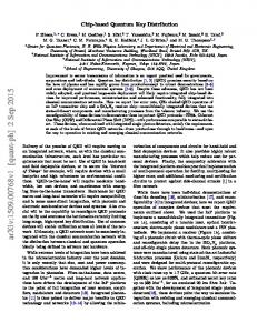
In the following, we describe the QKD schemes in details, see Fig. 1. Alice and Bob independently and ran-

FIG. 1: (Color online) Basic setup of P1 and P2 protocols. For simplicity, we consider the polarization encoding scheme. Alice (Bob) randomly prepares two (three) settings {A1 , A2 } ({B0 , B1 , B2 }) of quantum states with phase randomized WCPs. Charlie performs Bell state measurement and the measurement results are publicly announced. A successful Bell state measurement corresponds to the observa  tion of only two of four detectors being clicked. ψ + = √ a click in D1H and D1V , or 1/ 2(|HV i + |V Hi represents  √ D2H and D2V , while ψ − = 1/ 2(|HV i − |V Hi) represents a click in D1H and D2V , or D2H and D1V .

domly prepare quantum states with phase randomized WCPs in two settings {A1 = σz ,√A2 = σx } and three√settings {B0 = σz , B1 = (σz + σx )/ 2, B2 = (σz − σx )/ 2}, respectively. Then they send each pulse to an untrusted third party Charlie, who can be anybody, even the eavesdropper Eve. Charlie carries out a partial Bell state measurement (BSM). As is known, we cannot completely distinguish four Bell states simultaneously through singly using linear optical element. In this paper we can only unambiguously distinguish two Bell states {|ψ + i,|ψ − i} (Fortunately, the identification of one Bell state is adequate to prove security). Charlie announces through a public channel whether he has received a Bell state and which Bell state he has received. Alice and Bob keep the raw data of successful BSM results and discard the rest. The Bell value can be estimated from the raw data of quantum states sent by Alice’s and Bob’s two settings (bases) {A1 , A2 } and {B1 , B2 }, respectively. They postselect the results as a raw key when Alice and Bob choose setting A1 and B0 , respectively (here, A1 = B0 = σz ). Decoy-state techniques are employed [19–21] to estimate the yield, bit error rate and Bell value, given that both Alice and Bob send out single-photon states (untagged portion). One party needs to carry out a bit flip to his or her raw data to guarantee that their raw key is correctly correlated. Then they perform error-correction and privacy amplification with one-way classical postprocessing to extract secure keys.

3 IV.

by

SECURITY ANALYSIS

In this section, we present a brief description of P1’s and P2’s security against collective attacks and the main results of secure key rate. Here, we focus on collective attacks where Eve adopts the same attack to each system of Alice and Bob. For the first QKD protocol, P1, only signals originated from single-photon pulses emitted by both Alice and Bob are guaranteed to be secure while Eve’s information is restricted by the Holevo bound [4, 10]. Since the WCPs’ phase randomization makes the emitted quantum states of Alice and Bob into a classical mixture of states, it enables Alice and Bob to tag each pulse in principle though they do not need to do so in practice [28]. It is assumed that Eve competely knows the information from the multiphoton components (tagged portion). Then the information of Eve is composed of two portions, namely tagged and untagged portion, which can be written as (see Appendix A for more details) untag (A1 : E) χ1 (A1 : E) = χtag 1 (A1 : E) + χ1   S11 Z Z BZ √ = (QZ − Q ) + Q H e + . µν 11 11 11 2 2 (1) The mutual information between Alice and Bob, considering that the error-correction will leak extra information, is given by Z Z I1 (A1 : B0 ) = QZ µν − Qµν f H(Eµν ).

(2)

The secure key rate of P1 (per joint signal state emitted by Alice and Bob simultaneously in σz basis) can be written as R1 = I1 (A1 : B0 ) − χ1 (A1 : E)   h (3) S11 i BZ Z √ + 1 − H e = QZ − QZ 11 11 µν f H(Eµν ), 2 2 Z where QZ µν and Eµν , the overall gain and quantum bit error rate (QBER), can be directly obtained from the experimental results. The subscript µν means that Alice and Bob send out WCPs with intensity µ and ν, respectively. For the single-photon states, the gain QZ 11 , bit error rate eBZ 11 and the Bell value S11 can be estimated by the decoy-state method. Here, the parameter f is the error correction efficiency (we take the value f = 1.16 in our simulation), and H(e) = −e log2 (e)−(1−e) log2 (1−e) is the binary Shannon entropy function. For QKD protocol P2, the multiphoton components are tagged whose information will be fully leaked to Eve [28]. Only signals originated from single-photon pulses emitted by both Alice and Bob are the untagged portion which can be extracted as secure keys. For the untagged portion, we use the min-entropy to bound Eve’s knowledge of the secure keys, which has been applied to analyze security in Refs. [11, 27]. Details of this part can be found in Appendix B. The secure key rate of P2 is given

R2 = I2 (A1 : B0 ) − χ2 (A1 : E) ! r h i 2 S11 Z Z = Q11 1 − log2 1 + 2 − − QZ µν f H(Eµν ). 4 (4) Z The second term QZ f H(E ) quantifies the amount of µν µν information needed for the error-correction. The non  p 2 /4 QZ , trivial part of our bound is log2 1 + 2 − S11 11 which quantifies Eve’s information. When the phases of the WCPs sent by Alice and Bob are fully randomized, the density matrix of the quantum states should be written as Z 2π ∞ X µn dθ √ iθ √ iθ | µe ih µe | = e−µ |nihn|, (5) ρ= 2π n! 0 n=0 where θ and µ are the phase and intensity of the coherent states, respectively. Then the quantum channel can be considered as a photon number channel [20]. The overall gain and QBER in σz basis can be given by CZ EZ QZ µν = Qµν + Qµν =

∞ X ∞ X µn ν m −µ−ν Z e Ynm , n!m! n=0 m=0

Z CZ EZ Eµν QZ µν = ed Qµν + (1 − ed )Qµν ∞ X ∞ X µn ν m −µ−ν BZ Z e enm Ynm , = n!m! n=0 m=0

(6) Z where Ynm (eBZ ) is the yield (bit error rate), given that nm Alice and Bob send out n-photon and m-photon pulse, EZ respectively. QCZ µν (Qµν ) is the total gain of a successful BSM when the polarization of the pulses sent by Alice and Bob are different (the same) in σz basis, which represents a correct (false) measurement result. ed represents the overall misalignment-error probability of the system. The Bell value S11 is given by S11 =

1 ψ− ψ− ψ+ , ) = S11 (S11 + S11 2

ψ ψ ψ ψ = hA2 B2 iψ S11 11 − hA2 B1 i11 − hA1 B2 i11 − hA1 B1 i11 , (7) ψ+ ψ− because of symmetry. In our = S11 where we use S11 simulation, the expectation of single-photon states hAk ⊗ − ψ− Bl iψ 11 = hAk Bl i11 results from the successful projection into the Bell state |ψ − i with appropriate setting of Ak and Bl , where k, l ∈ {1, 2}. So the expectation is given by −

−

−

−

−

hAk Bl iψ 11 =(1 − 2ed ) −

− YV11ψ − YH11ψ + YV11ψ YH11ψ A HB A VB A VB A HB

×

l

k

l

k

−

−

−

−

l

k

l

k

YH11ψ + YV11ψ + YH11ψ + YV11ψ Ak HBl Ak VBl Ak VBl Ak HBl (8) − − is a yield. The superscript 11ψ reprewhere YH11ψ Ak VBl sents that Charlie obtains a Bell state |ψ − i successfully, −

−

−

−

,

4

10-5 10-7 10-9 10-11 0

50

100

150

200

250

300

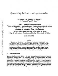
Standard fiber link HkmL FIG. 2: (Color online) The secure key rates in asymptotic case. Asymptotic case means that Alice and Bob use infinite number of decoy states and send Charlie infinite data signals. We use the following practical experimental parameters: the detection efficiency ηd of Charlie is 40%, the intrinsic loss coefficient β of the standard telecom fiber channel is 0.2 dB/km, the overall misalignment-error probability ed of the system is 1.5%, the background count rate pd is 3 × 10−6 , the intensity of signal state µ is 0.3.

SIMULATION RESULTS

In this section, we analyze the behavior of the secret key rates of P1 and P2 provided in Eq. (3) and Eq. (4), respectively. In our simulation, the loss of fiber-based channel is 0.2 dB/km. For simplicity, we assume that all detectors are identical (i.e., they have the same detection efficiency and background count rate), and their background count rate, to a good approximation, is independent of incoming signals. We assume that the detection efficiency of Charlie is 40% and the background count rate is 3 × 10−6. We use an intrinsic error rate that represents the misalignment and instability of the optical system. Furthermore, the security bound is fixed to be ǫ = 10−10 . The secure key rates of P1 and P2 in the asymptotic case are shown in Fig. 2 with blue dashed curve and black dashed curve, respectively. Meanwhile, we also present the simulation result of the MDI-QKD [16] with the red solid curve. We can see clearly that the secure key rate and secure distance of P1 are the same as MDI-QKD’s in the asymptotic case. The reason lies in that the security proof based on entanglement distillation purification is equivalent to direct information-theoretic arguments with one-way classical communications. The secure key rate and secure distance of P2 are both less than P1’s, since P2 requires fewer security assumptions, i.e., we do not require that Alice and Bob perfectly characterize their encoded quantum states. In practice, we need to consider a finite number of decoy states. The simulation results using linear programming and analytical method with vacuum+decoy states in asymptotic-data case (finite-data case) are shown in Fig. 3 (Fig. 4). Notice that the key rates using the analytical method almost overlap with the one using linear programming in Fig. 3 and Fig. 4. In the asymptotic-

0.001 Key rate Hper pulseL

V.

0.001 Key rateHper pulseL

given that both Alice and Bob send out single-photon states. The subscript HAk VBl represents the joint quantum state that Alice sends out a positive eigenvalue corresponding to the eigenstate of setting Ak while Bob sends out a negative eigenvalue corresponding to the eigenstate of setting Bl . Z We present two methods to obtain Y11 , eBZ 11 and S11 , the relevant parameters which are needed to evaluate the key rate formula above, given that Alice and Bob send Charlie a finite number of signals and use a finite number of decoy states. We use the standard error analysis method [29, 30] to solve this problem (a rigorous estimation can be acquired by using large deviation theory, i.e., the Chernoff bound [31]). More precisely, we combine linear programming and analytical method, respectively, with two decoy states, to estimate all the lower Z bounds of Y11 , eBZ 11 and S11 within single-photon states. Importantly, our methods are valid for arbitrary photonnumber distribution of signals sent by Alice and Bob. To get more details of this part, please see Appendix C.

10-5 10-7 10-9 10-11

0

50

100

150

200

250

300

Standard fiber link HkmL

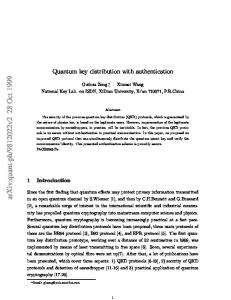
FIG. 3: (Color online) The secure key rates with two decoy states in asymptotic-data case. The intensities of signal state µ and one decoy state ν are 0.3 and 0.01, respectively, while the other decoy state is a vacuum state. We emphasize that the key rates with analytical method of Appendix C almost overlap with the one with linear programming, which shows that the analytical method provides an excellent estimation. The estimation using two decoy states gives a secure key rate which is nearly the same as the one using infinite decoy states. Therefore, two decoy states (vacuum+decoy) are enough for a near-optimal estimation, no matter how many decoy states are added, the secure key rate cannot be improved too much. In the asymptotic-data and two decoy states case, the security distances of P1 and P2 are more than 200 km.

data case (Fig. 3), the blue (black) solid curve represents the secure key rate of P1 (P2) under linear programming, while the red (green) dashed curve represents the secure key rate of P1 (P2) under analytical method. Comparing Fig. 2 with Fig. 3, we can see clearly that the key rates with two decoy states (vacuum+decoy) are close to the

5 corresponding ones with infinite number of decoy states. In finite-data case (Fig. 4), the statistical fluctuations are

ACKNOWLEDGMENTS

This work was supported by the NNSF of China under Grant No. 61125502, the National Fundamental Research Program under Grant No. 2011CB921300, the CAS and the National High Technology Research and Development Program of China.

0.001 Key rate Hper pulseL

VII.

10-5 10-7

Appendix A: HOLEVO BOUND

10-9 10-11 0

50

100

150

Standard fiber link HkmL

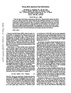
FIG. 4: (Color online) The secure key rates with statistical fluctuations. The intensities of signal state µ and one decoy state ν are 0.3 and 0.01, respectively, while the other decoy state is a vacuum state. The finite data is N = 1014 , the secure bound is ǫ = 10−10 . In the finite-data and two decoy states case, the security distance of P1 is more than 150 km, and the security distance of P2 is more than 110 km.

simulated using the standard error analysis method [29]. For simplicity, we assume that Alice and Bob send same number of pulses for all µAk ⊎ νBl channels, denoted by N (an efficient parameter optimization method can be found in [32]). Here µAk ⊎ νBl is defined as the case that Alice sends out WCPs of intensity µ with setting Ak while Bob sends out WCPs of intensity ν with setting Bl , where k ∈ {0, 1}, l ∈ {0, 1, 2}. In the finite-data and two decoy states cases, the security distance of P1 (P2) is more than 150 km (110 km).

Without loss of generality, the BB84 protocol implies that one can compute the bound by restricting consideration to collective attacks [4]. Considering the collective attacks, the final density matrix of Alice and Bob’s joint quantum state can be given by ρAB =λ1 |φ+ ihφ+ | + λ2 |φ− ihφ− | + λ3 |ψ + ihψ + | + λ4 |ψ − ihψ − |, with

P4

i=1

λi = 1. The four Bell states

1 |φ+ i = √ (|HHi + |V V i) = 2 1 |φ− i = √ (|HHi − |V V i) = 2 1 + |ψ i = √ (|HV i + |V Hi) = 2 1 |ψ − i = √ (|HV i − |V Hi) = 2

CONCLUSION

In summary, we have proposed two QKD protocols, P1 and P2, inspired by E91 and MDI-QKD protocols. As to P1, the security assumptions and the secure key rate in asymptotic case are the same as MDI-QKD’s. More importantly, in the security proof of P2, Alice and Bob’s perfectly characterizing encoded quantum states is not required. Thus, P2 is more resistant to source-side attacks compared with MDI-QKD. The simulation results show that P2 is more practical using conventional laser sources and decoy-state method instead of the singlephoton sources. P2 depends less on device but keeps a high secure key rate and long transmission distance. Moreover, the Bell value can be estimated accurately with conventional laser sources and finite-number decoy states method. We believe that this technique can be used in other fields of quantum information processing. The full parameter optimization of P1 and P2 needs to be done in the future.

1 √ (|++i + |−−i), 2 1 √ (|+−i + |−+i), 2 (A2) 1 √ (|++i − |−−i), 2 1 √ (|−+i − |+−i), 2

constitute a complete orthogonal basis in twodimensional Hilbert space. |φ± i (|φ+ i, |ψ + i) are perfectly correlated in σz (σx ) basis, while |ψ ± i (|φ− i, |ψ − i) are perfectly anticorrelated. Therefore, the bit error rates in σz and σx basis are given by eBZ = λ3 + λ4 ,

VI.

(A1)

eBX = λ2 + λ4 .

(A3)

The phase error rates in the two bases are eP Z = λ2 + λ4 = eBX ,

eP X = λ3 + λ4 = eBZ . (A4)

The secure key rate of the entanglement distillation purification-based QKD using one-way classical communications is [33, 34] REDP = 1 − H(eBZ ) − H(eP Z ) = 1 − H(eBZ ) − H(eBX ). (A5) Here, we use Holevo bound to estimate Eve’s information [35, 36], 1 1 χ(A : E) = S(ρE ) − S(ρE|0 ) − S(ρE|1 ) 2 2 = H(eBX ),

(A6)

and the secure key rate is RInf = I(A : B) − χ(A : E)

= 1 − H(eBZ ) − H(eBX ) = REDP .

(A7)

6 We can see that the security proof based on entanglement distillation purification is equivalent to direct information-theoretic arguments with one-way classical communications. The Bell operator can be written as B = A1 ⊗ B1 + A1 ⊗ B2 + A2 ⊗ B1 − A2 ⊗ B2 √ = 2(σz ⊗ σz + σx ⊗ σx ).

(A9)

Instead of using the bit error rate eBX in σx basis, the parameter from which Eve’s information is inferred is the average Bell value S and the √ bit error rate eBZ in σz BX BZ basis, i.e., e =1−e − S/2 2. Consider that Alice and Bob encode their bits in the polarization degrees of freedom of phase-randomized WCPs. The information of Eve with two portions [28], i.e., tagged and untagged portion, can be written as untag χ1 (A1 : E) = χtag (A1 : E) 1 (A1 : E) + χ1   S11 Z Z BZ √ = (QZ − Q ) + Q H 1 − e − µν 11 11 11 2 2   S11 Z Z BZ √ , = (QZ − Q ) + Q H e + µν 11 11 11 2 2 (A10) where the superscripts tag and untag represent tagged portion and untagged portion, respectively. The mutual information between Alice and Bob, considering that the error-correction will leak extra information, is given by Z Z I1 (A1 : B0 ) = QZ µν − Qµν f H(Eµν ).

(A11)

Finally, the secure key rate of P1 is given by R1 = I1 (A1 : B0 ) − χ1 (A1 : E)   h S11 i BZ Z Z = Q11 1 − H e11 + √ − QZ µν f H(Eµν ). 2 2 (A12) Appendix B: MIN-ENTROPY

In this part, the goal is to guarantee the security proof of P2 although removing the assumption that encoded quantum states need to be characterized perfectly. Obviously, the first five assumptions in section II are also required in the security proof of DI-QKD. The secure key rate of DI-QKD [11] is DI DI (A1 |E) − Hcon (A1 |B0 ), R = Hmin

DI Hmin (A1 |E) = −log2 Pguess (a),

DI Hcon (A1 |B0 ) = H(eBZ ).

(B2)

(A8)

Thus, the Bell value is given by [10] S = T r(BρAB ) √ = 2T r((σz ⊗ σz + σx ⊗ σx )ρAB ) √ = 2 2(λ1 − λ4 ) √ = 2 2(1 − eBZ − eBX ).

where

(B1)

DI In above equations, Hmin (A1 |E) is the (quantum) minentropy, which will be used for restricting the knowledge of Eve. By employing privacy amplification, we are able to make Eve’s information arbitrarily small. DI Hcon (A1 |B0 ) is the conditional Shannon entropy which quantifies the amount of information needed for errorcorrection. a is the output (eigenvalue) of setting {A1 , A2 }, and Pguess (a) is the maximal guessing probability which is used for quantifying the degree of unpredictability of Alice’s measurement output a. The following bound will hold in Bell’s inequality [37]

1 1 Pguess (a) ≤ + 2 2

r

2−

S2 . 4

(B3)

In the DI-QKD scheme, the loophole-free Bell test can ensure QKD security against untrusted detectors and arbitrarily dimensional quantum systems. P2 can be regarded as the modified time-reversed E91 and it is naturally immune to all possible detection-side attacks. The quantum states of P2 are required to be prepared in the two-dimensional Hilbert space, because the security of high-dimensional quantum states will not be guaranteed (for example, the four-dimensional separable state will have the property of two-dimensional maximally entangled state in Ref. [10]). Therefore, we can use the measurement data to calculate the Bell value with the assumption that the Hilbert space of quantum state preparation is two-dimensional. We use the min-entropy to bound Eve’s information with the untagged portion

  2 dim χuntag (A1 : E) = QZ 11 1 − Hmin (A1 |E) 2 ! r 2   1 1 S11 Z , + ≤ Q11 1 + log2 2− 2 2 4 (B4) where the superscript 2 dim represents that the Hilbert space of quantum systems is two-dimensional. From the analysis above, it is not necessarily required that Alice and Bob perfectly characterize their encoded quantum states. Eve will acquire more information because the dimension of DI-QKD’s quantum systems is arbitrary. Then the following inequality will hold,

2 dim DI (A1 |E) ≥ Hmin (A1 |E). Hmin

(B5)

7 The secure key rate of P2 is given by R2 =I2 (A1 : B0 ) − χ2 (A1 : E)

untag =I2 (A1 : B0 ) − [χtag (A1 : E)] 2 (A1 : E) + χ2

Z Z Z Z ≥QZ µν − Qµν f H(Eµν ) − (Qµν − Q11 ) ! r h i 2 1 1 S11 Z − Q11 1 + log2 2− + 2 2 4 ! r i h 2 S11 Z 2 − − QZ 1 + =QZ 1 − log 2 µν f H(Eµν ). 11 4 (B6)

=

QCZ µi νj

+

QEZ µi νj

∞ X ∞ X µni νjm −µi −νj Z = Ynm , e n!m! n=0 m=0

EZ CZ EµZi νj QZ µi νj = ed Qµi νj + (1 − ed )Qµi νj

=

2V

gain and error

Now, we evaluate the overall gain and QBER. Alice and Bob prepare phase-randomized WCPs with intensity µi and νj , respectively. The overall gain and QBER in σz basis (Alice chooses setting A1 and Bob chooses setting B0 ) can be written as [30] QZ µi νj

q q E E iφa p µi ηa νj ηb νj ηb π iφb iφb e cos 3π 2 + cos 8 e 2 8 e 2 1V q 1H E iφa p µi ηa νj ηb π iφb ⊗ e 2 − cos 8 e 2 2H q E νj ηb 3π iφb ⊗ − cos 8 e , 2

(C4) where the four detection modes are 1H, 1V , 2H and 2V . Therefore, the detection probabilities for the four detectors are given by

BZ Appendix C: ESTIMATE QZ 11 , e11 and S11

1.

where φa and φb are the overall randomized phases, while |Hi (|V i) is a positive (negative) eigenvalue corresponding to the eigenstate of σz basis. Then the quantum state passing through the beam splitter and four polarization beam splitters is given by

∞ ∞ X X µni νjm −µi −νj BZ Z enm Ynm , e n!m! n=0 m=0

D1H D1V D2H D2V

√ √ eiφa µi ηa + cos π8 eiφb νj ηb 2 √ | ), = 1 − (1 − pd ) exp(−| 2 iφb √ cos 3π νj ηb 2 8 e √ = 1 − (1 − pd ) exp(−| | ), 2 √ √ eiφa µi ηa − cos π8 eiφb νj ηb 2 √ | ), = 1 − (1 − pd ) exp(−| 2 iφb √ − cos 3π νj ηb 2 8 e √ = 1 − (1 − pd ) exp(−| | ). 2 (C5) µ ν ψ−

(C1)

where  µi ηa  2 −ω 2 1 − (1 − p )e− 2 QCZ d µi νj =2(1 − pd ) e ν j ηb   (C2) × 1 − (1 − pd )e− 2 ,  ω 2 −ω EZ − Qµi νj =2pd (1 − pd ) e 2 I0 (2x) − (1 − pd )e 2 .

In the above equations, pd is the background count rate, I0 (2x) is the modified Bessel function of the first kind, ed represents the misalignment-error probability, and √ µi νj ηa ηb ω = µi ηa + νj ηb , x = . η = η = ηd × 10−βL/20 a b 2 is the total efficiency including channel transmittance efficiency 10−βL/20 and detection efficiency ηd . Considering the symmetric scenario, the distance between Alice (Bob) and Charlie is L/2. Now, we focus on the joint quantum state. Alice sends out a positive eigenvalue corresponding to the eigenstate |HA1 i = |Hi of setting A1 and Bob sends out a positive eigenvalue corresponding to the eigenstate |HB1 i = cos π8 |Hi + cos 3π 8 |V i of setting B1 , i.e.,   π √ √ |HA1 i ⊗ |HB1 i = eiφa µi ηa H ⊗ cos eiφb νj ηb H 8 
3π iφb √ νj ηb V , + cos e 8 (C3)

The gain QHiAj HB is defined as the probability that Al1 1 ice sends out a positive eigenvalue corresponding to the eigenstate |HA1 i = |Hi of setting A1 with the intensity µi , while Bob sends out a positive eigenvalue corresponding to the eigenstate |HB1 i = cos π8 |Hi+cos 3π 8 |V i of setting B1 with the intensity νj . Meanwhile, Charlie has a successful Bell state |ψ − i measurement event. Therefore, µ ν ψ− QHiAj HB 1 1

Z 2π 1 1 = D1H D2V (1 − D2H )(1 − D1V ) 2π 0 4  + D2H D1V (1 − D1H )(1 − D2V ) dφ, (C6)

µ ν ψ−

where QHiA j HB is averaged over random phases φa and 1 1 φb , φ = φa − φb . By substituting Eq. (C5) into Eq. (C6), we have

µ ν ψ−

QHiAj HB = 1

1

∞ X ∞ X µni νjm −µi −νj nmψ− YHA HB e 1 1 n!m! n=0 m=0

ω π 1 1 = (1 − pd )2 e− 2 I0 (2x cos ) + (1 − pd )4 e−ω 2 8 2 2µi ηa +(1+cos2 π )νj ηb 1 8 2 − (1 − pd )3 e− 2 µi ηa +(1+cos 2 3π )νj ηb π 1 8 2 I0 (2x cos ). − (1 − pd )3 e− 2 8 (C7)

8 According to the above procedures, we can also obtain µ ν ψ−

QHiAj VB = 1

1

∞ X ∞ X µni νjm −µi −νj nmψ− YHA VB e 1 1 n!m! n=0 m=0

ω 1 1 3π (1 − pd )2 e− 2 I0 (2x cos ) + (1 − pd )4 e−ω 2 8 2 2µ ηa +(1+cos 2 3π )νj ηb 1 8 3 − i 2 − (1 − pd ) e 2 µi ηa +(1+cos2 π )νj ηb 3π 1 8 2 I0 (2x cos ), − (1 − pd )3 e− 2 8 (C8)

=

µ ν ψ−

∞ X ∞ X µni νjm −µi −νj nmψ− YHA HB e 1 2 n!m! n=0 m=0 √ ω 1 π 3π = (1 − pd )2 e− 2 I0 ( 2x(cos − cos )) 2 8 8 3 µ η +(1+cos 2 π )ν η √ j b 3π 1 2 i a 8 2 I0 ( 2x cos ) − (1 − pd )3 e− 2 8 3 µ η +(1+cos 2 3π )ν η √ j b π 1 2 i a 8 2 I0 ( 2x cos ) − (1 − pd )3 e− 2 8 1 4 −ω + (1 − pd ) e , 2 (C9)

QHiAj HB = 1

2

∞ X ∞ X µni νjm −µi −νj nmψ− YHA VB e 1 2 n!m! n=0 m=0 √ ω 1 π 3π = (1 − pd )2 e− 2 I0 ( 2x(cos + cos )) 2 8 8 3 µ η +(1+cos2 π )ν η √ j b 3π 1 2 i a 8 2 I0 ( 2x cos ) − (1 − pd )3 e− 2 8 3 µ η +(1+cos2 3π )ν η √ j b 1 π 2 i a 8 2 − (1 − pd )3 e− I0 ( 2x cos ) 2 8 1 4 −ω + (1 − pd ) e , 2 (C10)

µ ν ψ−

QHiAj VB = 1

2

and

rate in σz basis with single-photon states are given by [30]  ηa ηb + (2ηa + 2ηb − 3ηa ηb )pd 2  + 4(1 − ηa )(1 − ηb )p2d , ηa ηb Z Z 2 , eBZ 11 Y11 =e0 Y11 − (e0 − ed )(1 − pd ) (1 − 2pd ) 2 (C13) ψ− where e0 = 12 . The Bell value S11 of single-photon states is given by Z Y11 =(1 − pd )2

ψ ψ ψ ψ = hA2 B2 iψ S11 11 − hA2 B1 i11 − hA1 B2 i11 − hA1 B1 i11 , (C14) where

hAk Bl iψ 11 =(1 − 2ed ) −

×

µ ν ψ−

1 −

µ ν ψ QHiA j VB 1 1 µ ν ψ QHiAj HB 1 2 −

µ ν ψ

−

1 −

1

µ ν ψ−

=

µi νj ψ QVA 1 HB1

=

µi νj ψ QVA 2 VB1 −

µ ν ψ

−

=

µ ν ψ QHiAj VB 2 1

=

µ ν ψ QHiAj VB 2 2 −

µ ν ψ

1

−

1

1

= =

µi νj ψ − QVA , 2 HB2

1

2

1

2

2

2

−

1

YH11ψ = A HB 2

The gain of single-photon states (untagged portion) in σz basis, QZ 11 , is given by −µ−ν Z QZ Y11 . 11 = µνe

(C12)

For the asymptotic case (with infinite number of decoy states and infinite data length), the yield and bit error

− YH11ψ Ak VBl

k

+

l

− YV11ψ Ak HBl

(C15)

π pd (1 − pd )2 [1 − (1 − 2pd )(1 − ηa ) 8 4 pd 3π × (1 − ηb )] + cos2 (1 − pd )2 8 8 × [(2 − ηa − ηb ) + 2(1 − pd )(1 − ηa )(1 − ηb )]

3π pd (1 − pd )2 [1 − (1 − 2pd )(1 − ηa ) 8 4 π pd cos2 (1 − pd )2 × (1 − ηb )] + 8 8 × [(2 − ηa − ηb ) + 2(1 − pd )(1 − ηa )(1 − ηb )] +

2

Asymptotic case

+

−

l

(1 − pd )2 π cos2 [pd (ηa + ηb ) 8 8 + (1 − 2pd )ηa ηb + 2p2d (1 − ηa )(1 − ηb )], (C17)

(C11)

−

2.

− YV11ψ Ak VBl

k

YH11ψ = cos2 A VB

i j i j i j QHiA j VB = QVA HB = QHA HB = QVA VB . 2

+

−

l

(1 − pd )2 3π cos2 [pd (ηa + ηb ) 8 8 + (1 − 2pd )ηa ηb + 2p2d (1 − ηa )(1 − ηb )], (C16)

µ ν ψ−

−

− YH11ψ Ak HBl

k

+

2

µi νj ψ − QVA , 1 HB2

−

l

YH11ψ = cos2 A HB

µ ν ψ−

2 −

1

k

k, l ∈ {1, 2}. Thereinto,

i j i j i j QHiAj HB = QVA VB = QHA HB = QVA VB , 1

YH11ψ + YV11ψ − YH11ψ − YV11ψ A HB A VB A VB A HB −

1

µ ν ψ−

−

−

−

−

−

1

pd (1 − pd )2 [1 − (1 − 2pd )(1 − ηa )(1 − ηb )] 8 π 3π 2 pd ) (1 − pd )2 [(2 − ηa − ηb ) + (cos + cos 8 8 8 + 2(1 − pd )(1 − ηa )(1 − ηb )] π 3π 2 (1 − pd )2 (cos − cos ) [pd (ηa + ηb ) 16 8 8 + (1 − 2pd )ηa ηb + 2p2d (1 − ηa )(1 − ηb )], (C18) +

,

9 pd (1 − pd )2 [1 − (1 − 2pd )(1 − ηa )(1 − ηb )] 8 π 3π 2 pd ) (1 − pd )2 [(2 − ηa − ηb ) + (cos − cos 8 8 8 + 2(1 − pd )(1 − ηa )(1 − ηb )]

YH11ψ = A VB −

1

2

(1 − pd )2 π 3π 2 (cos + cos ) [pd (ηa + ηb ) 16 8 8 2 + (1 − 2pd )ηa ηb + 2pd (1 − ηa )(1 − ηb )], (C19)

YH11ψ = YV11ψ = YH11ψ = YV11ψ , A HB A VB A HB A VB −

−

1

1

− YH11ψ A1 VB1

YH11ψ A2 HB1 −

= =

−

1

1

− YV11ψ A1 HB1

YV11ψ A2 VB1 −

−

2

1

=

− YH11ψ A1 VB2

=

YH11ψ A2 VB2 −

2

1

=

− YV11ψ , A1 HB2

=

− YV11ψ , A2 HB2

(C20)

2

−

1

2

3.

−

1

2

ψ S11

−

L

−

2

2

2

In practical demonstrations, the length of the raw key is finite, which will induce statistical fluctuations for the parameter estimation. Here, we consider the effect of finite length raw key based on standard error analysis ψ− Z method [29, 30]. The estimations of Y11 , eBZ 11 and S11 are constrained optimization problems, which are linear and can be efficiently solved by linear programming [30, 32]. Now, we consider an analytical estimation method with two decoy states [38], µ2 = ν2 > µ1 = ν1 > µ0 = ZL ν0 = 0. The lower bound of Y11 , the upper bound of ZU BZL Y11 and the lower bound of e11 are given by ZL Y11

ZU Y11 ≤

≥2(1 − 2ed)   − L 11ψ − U 11ψ − U 11ψ − L YH11ψ − Y − Y Y H V H H H V H B1 a1 b1 A1 B1 A2 A2 B1 , ×  11ψ− U −U + 11ψ − U 11ψ − U + Y YHA HB + YH11ψ Y HA2 VB1 HA2 HB1 A1 VB1 1 1 (C24)

where

Finite decoy-state case

h 1 Z ≥ 2 2 µ3 e2µ1 QZ µ1 µ1 + Q00 µ2 µ1 (µ2 − µ1 ) 2
µ1 Z 3 2µ2 Z Qµ2 µ2 − eµ1 QZ µ1 0 − e Q0µ1 − µ1 e i
µ2 Z µ2 Z + QZ 00 − e Qµ2 0 − e Q0µ2 ,

i

(C23) Combining Eq. (C11) and Eq. (C20), we can use the folψ− , lowing equations to estimate the lower bound of S11

YH11ψ = YV11ψ = YH11ψ = YV11ψ . A VB A HB A HB A VB −

h µ32 e2µ1 EµZ1 µ1 QZ µ1 µ1

Z µ1 Z Z Z + E00 Q00 − eµ1 EµZ1 0 QZ µ1 0 − e E0µ1 Q0µ1 h Z Z − µ31 e2µ2 EµZ2 µ2 QZ µ2 µ2 + E00 Q00 ) i Z Z µ2 Z µ2 Z − e Eµ2 0 Qµ2 0 − e E0µ2 Q0µ2 .

+

and

(

1 ≥ 2 2 ZU µ2 µ1 (µ2 − µ1 )Y11

eBZL 11

L ≥ YH11ψ A VB

1

−

k

l

µ22 µ21 (µ2 − µ1 ) − − eµ1 QµH1A0ψVB l k

h − − µ32 e2µ1 QµH1Aµ1VψB + Q00ψ HA VB −

− µ31 e2µ2 QµH2Aµ2VψB + Q00ψ HA −

−e

U YH11ψ ≤ A HB −

l

k

− QµH2A0ψVB l k

−e

µ2

VBl

i

−
2ψ Q0µ HAk VBl

, (C25)

− 1 h 2µ1 µ1 µ1 ψ− e QHA HB + Q00ψ HBl H 2 A l k k µ1

−e

µ1

l

−

k

l

k

µ2

k

l

k

−
1ψ eµ1 Q0µ HAk VBl

− QµH1A0ψHB l k

−e

µ1

− 1ψ Q0µ HAk HBl

i ,

(C26)

(C21)

 1  2µ1 Z µ1 Z µ1 Z e Qµ1 µ1 + QZ 00 − e Qµ1 0 − e Q0µ1 , 2 µ1 (C22)

[1] C. H. Bennett and G.Brassard, in Proceedings of IEEE International Conference on Computers, Systems, and Signal Processing (IEEE, New York, 1984), p. 175. [2] A. K. Ekert, Phys. Rev. Lett. 67, 661 (1991). [3] N. Gisin, G. Ribordy, W. Tittel, and H. Zbinden, Rev. Mod. Phys. 74, 145 (2002). [4] V. Scarani, H. Bechmann-Pasquinucci, N. J. Cerf, M. Duˇsek, N. L¨ utkenhaus, and M. Peev, Rev. Mod. Phys. 81, 1301 (2009). [5] Y. Zhao, C.-H. F. Fung, B. Qi, C. Chen, and H.-K. Lo,

U YH11ψ ≤ A VB −

k

l

− 1 h 2µ1 µ1 µ1 ψ− e QHA VB + Q00ψ V H 2 A l k k Bl µ1

i − − 1ψ − eµ1 QµH1A0ψVB − eµ1 Q0µ HA VB , k

l

k

(C27)

l

and k, l ∈ {1, 2}.

Phys. Rev. A 78, 042333 (2008). [6] F. Xu, B. Qi, and H.-K. Lo, New J. Phys. 12, 113026 (2010). [7] L. Lydersen, C. Wiechers, C. Wittmann, D. Elser, J. Skaar, and V. Makarov, Nature Photon. 4, 686 (2010). [8] H. Weier, H. Krauss, M. Rau, M. F¨ urst, S. Nauerth, and H. Weinfurter, New J. Phys. 13, 073024 (2011). [9] I. Gerhardt, Q. Liu, A. Lamas-Linares, J. Skaar, C. Kurtsiefer, and V. Makarov, Nature Commun. 2, 349 (2011). [10] S. Pironio, A. Acin, N. Brunner, N. Gisin, S. Massar, and

10 V. Scarani, New J. Phys. 11, 045021 (2009). [11] L. Masanes, S. Pironio, and A. Acn, Nature Commun. 2, 238 (2011). [12] C. C. W. Lim, C. Portmann, M. Tomamichel, R. Renner, and N. Gisin, Phys. Rev. X 3, 031006 (2013). [13] M. Giustina, A. Mech, S. Ramelow, B. Wittmann, J. Kofler, J. Beyer, A. Lita, B. Calkins, T. Gerrits, S. W. Nam, R. Ursin, and A. Zeilinger, Nature 497, 227 (2013). [14] B. G. Christensen, K. T. McCusker, J. B. Altepeter, B. Calkins, T. Gerrits, A. E. Lita, A. Miller, L. K. Shalm, Y. Zhang, S. W. Nam, N. Brunner, C. C. W. Lim, N. Gisin, and P. G. Kwiat, Phys. Rev. Lett. 111, 130406 (2013). [15] N. Gisin, S. Pironio, and N. Sangouard, Phys. Rev. Lett. 105, 070501 (2010). [16] H.-K. Lo, M. Curty, and B. Qi, Phys. Rev. Lett. 108, 130503 (2012). [17] E. Biham, B. Huttner, and T. Mor, Phys. Rev. A 54, 2651 (1996). [18] H. Inamori, Algorithmica 34, 340 (2002). [19] W.-Y. Hwang, Phys. Rev. Lett. 91, 057901 (2003). [20] H.-K. Lo, X. Ma, and K. Chen, Phys. Rev. Lett. 94, 230504 (2005). [21] X.-B. Wang, Phys. Rev. Lett. 94, 230503 (2005). [22] R. Ursin, F. Tiefenbacher, T. Schmitt-Manderbach, H. Weier, T. Scheidl, M. Lindenthal, B. Blauensteiner, T. ¨ Jennewein, J. Perdigues, P. Trojek, B. Omer, M. F¨ urst, M. Meyenburg, J. Rarity, Z. Sodnik, C. Barbieri, H. Weinfurter, and A. Zeilinger, Nature Phys. 3, 481 (2007). [23] X. Ma, C.-H. F. Fung, and H.-K. Lo, Phys. Rev. A 76, 012307 (2007). [24] J. Barrett, R. Colbeck, and A. Kent, Phys. Rev. Lett.

110, 010503 (2013). [25] M. Pawlowski and N. Brunner, Phys. Rev. A 84, 010302(R) (2011). [26] Z.-Q. Yin, C.-H. F. Fung, X. Ma, C.-M. Zhang, H.-W. Li, W. Chen, S. Wang, G.-C. Guo, and Z.-F. Han, Phys. Rev. A 88, 062322 (2013). [27] H.-W. Li, Z.-Q. Yin, W. Chen, S. Wang, G.-C. Guo, and Z.-F. Han, Phys. Rev. A 89, 032302 (2014). [28] D. Gottesman, H.-K. Lo, N. L¨ utkenhaus, and J. Preskill, Quant. Inf. Comput. 4, 325 (2004). [29] X. Ma, B. Qi, Y. Zhao, and H.-K. Lo, Phys. Rev. A 72, 012326 (2005). [30] X. Ma, C.-H. F. Fung, and M. Razavi, Phys. Rev. A 86, 052305 (2012). [31] M. Curty, F. Xu, W. Cui, C. C. W. Lim, K. Tamaki, and H.-K. Lo, Nature Commun. 5, 3732 (2014). [32] F. Xu, H. Xu, and H.-K. Lo, Phys. Rev. A 89, 052333 (2014). [33] C. H. Bennett, D. P. DiVincenzo, J. A. Smolin, and W. K. Wootters, Phys. Rev. A 54, 3824 (1996). [34] P. W. Shor and J. Preskill, Phys. Rev. Lett. 85, 441 (2000). [35] B. Kraus, N. Gisin, and R. Renner, Phys. Rev. Lett. 95, 080501 (2005). [36] R. Renner, N. Gisin, and B. Kraus, Phys. Rev. A 72, 012332 (2005). [37] S. Pironio, A. Ac´ın, S. Massar, A. Boyer de La Giroday, D. N. Matsukevich, P. Maunz, S. Olmschenk, D. Hayes, L. Luo, T. A. Manning, and C. Monroe, Nature 464, 1021 (2010). [38] F. Xu, M. Curty, B. Qi, and H.-K. Lo, New J. Phys. 15, 113007 (2013).