Keywords: Discrete Fourier Transform, measuring integral nonlinearity, ... nonlinearity, of an ADC from the output spectrum yielded by the DFT test. This is done ...
MEASUREMENT OF ADC INTEGRAL NONLINEARITY VIA DFT F. Adamo, F. Attivissimo, N. Giaquinto Laboratory for Electric and Electronic Measurements Department of Electrics and Electronics (DEE) – Polytechnic of Bari Via E. Orabona 4, 70125 Bari Abstract: the paper presents a new methodology, based on the Discrete Fourier Transform of the output, for measuring the integral nonlinearity of an ADC. The new method, unlike the usual histogram test, gives the best polynomial approximation (the “smooth part”) of the integral nonlinearity, which is responsible for the spurious harmonics above the ADC noise floor, and can be performed with great accuracy and repeatability with as few as 8,000 samples, irrespective the ADC resolution. This makes this test by far faster than the histogram test for high-resolution devices. Keywords: Discrete Fourier Transform, measuring integral nonlinearity, histogram test 1 INTRODUCTION A main issue in testing analog-to-digital converters (ADC’s) and ADC-based devices is, of course, determining the nonlinear input-output static characteristic, or, to say better, the deviation of the characteristic of the actual device from that of an ideal quantizer. The standard methodology for this type of measurement is the code density or histogram test [1]. This method is actually extremely accurate but it obliges to acquire a large number of samples, proportional to the number of output codes of the ADC under test. Proper execution of the test requires therefore a large amount of time, especially for ADC’s with low speed and high resolution (16 bits or more). Besides, the histogram test yields exclusively the ADC nonlinearity, and no information about noise or other error phenomena. The Discrete Fourier Transform (DFT) test of converters, on the contrary, is always very fast as it can be satisfactorily performed with four or eight thousands samples and Fast Fourier Transform (FFT) algorithms. This kind of test, moreover, yields information about both noise and distortion introduced in the conversion, and also about more complex events that are visible in the frequency domain (out-of-phase harmonics, for example, denote that dynamic nonlinearity or timebase distortion are present). Unfortunately the DFT test does not yield, unlike the histogram test, the complete static characteristic of the ADC, but only an indirect information, that is the harmonic distortion generated by the nonlinearity. This work presents and explain a procedure that derives the static characteristic, i.e. the integral nonlinearity, of an ADC from the output spectrum yielded by the DFT test. This is done by using a known theorem from nonlinear system theory and by introducing the distinction between “smooth” and “granular” nonlinearity. Simulations and experiments show that the methodology actually allows one to derive, in a fraction of the time required by the histogram test, an accurate measurement of the “smooth part” of the nonlinearity, which is the cause of the harmonics observable above the noise floor. Microscopic details of the integral nonlinearity, like missing codes, spikes, etc. (“granular part” of the nonlinearity) are not detected by the DFT test, which is the price to pay for the low number of samples employed. Knowledge of the smooth nonlinearity, however, appears to be sufficient and very useful for many practical applications, ranging from the evaluation of harmonic distortion effects on multi-tone input signals, up to the error correction for increasing the spurious-free dynamic range (SFDR).
2 THEORY Let us consider a nonlinear static system described by the real single-valued function y = g (x ) . If the input is a sinusoidal signal with null phase x (t ) = V cos ωt + C , the output is a periodic signal at the same frequency with generic shape, that can be therefore expanded in Fourier series:
y (t ) =
a0 + 2
∞
∑a
cos(nωt ) + bn sen( nωt )
n
(1)
n =1
The sine terms bn are in fact zero as, because of the zero phase of the sinusoidal input, the output y (t ) is an even function: x ( −t ) = x (t ) ⇒ y ( −t ) = g ( x ( −t )) = g ( x (t )) = y (t ) . The cosine terms an can be expressed, by substituting cos(ωt ) = z and with simple algebraic manipulations, in the form an =
2 π
1
g (Vz + C )C n ( z )
−1
1 − z2
∫
dz
(2)
where the terms C n (z ) are the Chebyshev polynomials of the first kind. In particular the identity C n (cos θ) = cos(nθ) must be exploited to derive (2). Another important property of these polynomials is that they are orthogonal with respect to the weight function 1 − x 2 : this implies that a generic function f (x ) can be expanded in a series of Chebyshev polynomials of the form f (x ) =
c0 + 2
∞
∑c C (x) n
n
(3)
n =1
where the coefficients c n are given by cn =
2 π
∫
1
f ( x )C n ( x )
−1
1− x 2
dx
(4)
By comparing equations (2) and (4) it is obvious that the terms an in the Fourier expansion of the output of g (x ) with zero-phase sinusoidal input do represent the terms of the expansion of g (Vx + C ) in Chebyshev polynomials series. Consequently, if the coefficients an are known, g (x ) is given by g( x ) =
a0 + 2
∞
∑ a C n
n =1
n
x −C V
(5)
This equation, that relates a nonlinear function with the spectrum of its output, has been known for a long time, but apparently it has been never employed in a procedure of ADC testing (it is useful, however, to read a recent paper [2] on the same topic of the present one). Indeed, under a strictly theoretical point of view, (5) is not applicable even to a simple ideal ADC, whose characteristic g (x ) is simply a staircase with a large number of equispaced discontinuity points. It is clear that such a function cannot be approximated by a polynomial of reasonable order: equation (5) is therefore not useful (and not encountered) in quantization theory. Application of (5) to ADC testing requires some additional consideration. The actual static characteristic g (x ) of an ADC can be seen, as shown in Fig. 1, as the cascade of a nonlinear smooth (that means here “without discontinuities”) function g s (x ) and an ideal quantization function quant (x ) , with a large number of discontinuities. A correct g s (x ) is any function such that | g s ( x ) − g ( x ) |≤ 0.5 LSB: in particular, a valid g s (x ) is a linear piecewise function connecting the points (t kid , t k ) , being t kid the threshold levels of the ideal quantizer and t k the threshold levels of the actual ADC. Therefore, measuring the actual threshold levels of an ADC, for example via an histogram test, is equivalent to finding the smooth function g s (x ) , that (contrary to the overall characteristic g (x ) ) seems to be approximable by a polynomial with reasonable accuracy. If one could have access to the output of g s (x ) before the quantization, application of (5) would be automatic. Having access only to the output of g ( x ) = quant (g s ( x )) , it is obvious to ask about the effect of quant (x ) on the output spectrum. Fortunately, this effect is not much important for ADC’s
with practical values of resolution (8 bits or higher). Strictly speaking, quantization adds further spurious harmonics that change in a hardly computable way the spectrum of g s (x ) : for example, as computed by Clavier, Panter e Grieg first [3], [4], if the input of quant (x ) is a sine wave, the output spectrum is
S 2n −1
1 = π
∞
∑ l =1
1 J 2n −1(2πlV / Q ) l
2
(6)
being n = 1,...,+∞ , Q the quantization step and J n the Bessel function of the first kind of order n. In practice, however, the harmonics similar to (6) generated by quant (x ) have very little effect on the harmonics generated by g s (x ) , as their overall power (about Q 2 / 12 ) is distributed in a very large number of spectral bins. For example, for an 8-bit ADC the first 750 harmonics must be taken into account to reach about 70% of the quantization error power [5]. The above considerations are readily verified by examining the DFT of the output in a practical ADC stimulated by a coherently sampled sine wave (Fig. 2). A moderate number of larger harmonics, due to a polynomial nonlinear function g s (x ) , is well visible above the “noise floor”, that is actually made, at least in part, of the harmonics (6) due to quant (x ) . The noise floor will not influence meaningfully the larger harmonics, provided the ADC resolution is not too small and the coherent sampling scheme is adopted, which guarantees that harmonics (6) are not distributed on a small number of spectral bins.
3 TEST METHOD On the basis of the mathematics and the general considerations illustrated above, a straigthforward algorithm for the fast measurement of the smooth transfer characteristic g s (x ) (i.e. the integral nonlinearity) of an ADC, via DFT analysis, can be easily formulated: 1) stimulate the ADC input with a sinusoidal signal, in which the spurious harmonics do not exceed those introduced by ideal quantization and given by (6); 2) select signal frequency, sampling frequency and duration of the sampling so that the output y (kTs ) , k = 0 : N − 1 embodies an integer number N p of periods, prime relative to the number N of samples; 3) start the acquisition of the distorted sine wave y (kTs ) approximately when the fundamental component has null phase; 4) evaluate the DFT: N −1
Y (i / NTs ) =
∑ y (kT )e
− j 2 πik / N
s
i = 0 : N −1
(7)
k =0
by means of a suitable FFT algorithm; 5) establish the maximum degree N h of the polynomial by which g s (x ) is to be approximated, and find the indexes i n = (nN p mod N ) with n = 0,...N h , where the harmonics of the fundamental sine wave are located; 6) evaluate the N h + 1 real coefficients: a n = 2Y (i n ) / N
n = 0,...N h ;
(8)
7) find the N h -degree polynomial that approximates g s (x ) using (5). This algorithm, of course, can be in practice sped up and improved with some artifices. First of all it is opportune to simplify and, if the case, to lower the degree of the polynomial g s (x ) by setting an = 0 when | Y (i n ) | is below a fixed threshold, that can be determined on the basis of the observed noise floor in the DFT (that includes quantization noise, thermal noise, and similar phenomena). Second, as
it is not likely to obtain in practice the coefficients
a n with exactly null imaginary part, as predicted by
theory, it is possible to cancel the effect of a small nonzero phase by assuming simply an = sign(Re(Y (i n )) ⋅ 2 | Y (i n ) | / N , instead of (8). It is possible, of course, to neglect the zero phase requirement on the fundamental of y (kTs ) , and correcting digitally the time shift in the time domain or in the frequency domain. Finally it must be highlighted that, if meaningful out-of-phase harmonics are observed, the no-memory model of the converter can no more be considered valid, and a lower signal and/or sampling frequency must be selected, in order to get the static part of the device characteristic.
4 SIMULATIONS The described test method for ADC’s has been firstly proven by simulating nonlinar ADC’s according the scheme shown in Fig. 1. The simulated nonlinear smooth transfer characteristic g s (x ) is a trascendent function, with oscillation of variable amplitude and a small trend: g s ( x ) = (1 + ∆G )x + ∆O + INLmax sin(10 πx / x FS ) ⋅ exp(sin(7 x / x FS ) − 1)
(9)
being ∆G the gain error, ∆O the offset error, INLmax the maximum integral nonlinearity error and x FS the full-scale range of the ideal quantizer (i.e. of the simulated ADC). This expression for g s (x ) has been chosen because it simulates in a rather realistic way a smooth nonlinearity, and there is not a trivial polynomial approximation for it. ADC’s with resolution of 8, 12, 16 and 20 bits have been simulated, so covering a wide range of resolutions. The following values have been employed for the parameters in (9): ∆G | x |max = 0.2 LSB, ∆O = −0.5 LSB, INLmax = 0.5 LSB. It is obvious that these values make the error g s ( x ) − x (the integral nonlinearity) of the same order of magnitude of the quantization error, just like is found in good real-world ADC’s. It is useful to examine Fig. 3, in which the overall ADC error g ( x ) − x = quant (g s ( x )) − x is plotted together with the wanted nonlinearity error g s ( x ) − x . In order to illustrate the capability of the proposed method due results of two sets of simulations are presented, the first relevant to a 4,096 points DFT and the second to an 8,192 DFT. It is evident that such a small number of samples could be scarcely sufficient for the 8-bit ADC using the histogram test. In all the simulations, N h = 20 has been chosen as maximum harmonic order (and therefore maximum degree of the polynomial approximation of g s (x ) ), and only the harmonics such that | Y (i n ) |2 / N > 10 ⋅ Q 2 / 12 have been considered in the computation of g s (x ) via (5). This threshold has come out to work well in the simple case considered in the simulations, when the noise floor is made only by the harmonics (6) due to ideal quantization. Figures 4 and 5 show the results of the simulated tests, comparing the true g s (x ) () with the estimation made via DFT in the case of 8-bit (ooo), 12-bit (xxx), 16-bit (+++) and 20-bit (***) ADC. The first figure is relevant to the 4,096 samples DFT while the second to the case of 8,192 samples. When using 4,096 samples the maximum error in estimating g s (x ) is about 0.16 LSB for the 16-bit ADC, and about 0.1 LSB for the others. When using 8,192 samples the maximum error comes out to be, in all cases, about 0.05 LSB. It can be inferred, also on the basis of other simulations not presented here for brevity, that the estimation error on g s (x ) decreases by increasing the number of DFT samples (in accordance with the simple considerations illustrated in section 2), while it is practically independent on the ADC resolution if it is not too low (< 6 bits). In this case the quantization error tends to be less uniformely distributed in the DFT bins and is more likely to interfere with the harmonics generated by g s (x ) . In all the other cases the estimation error is very small and, above all, independent on the resolution even if the same number of samples is taken, which is a big and important difference with respect to the histogram test.
5 EXPERIMENTAL RESULTS The proposed method for measuring the integral nonlinearity via DFT has been performed on actual digital instrumentation, comparing the results with those yielded by an histogram test executed with a very high number of samples (these results can be assumed to be the “true” nonlinearity
functions). The DFT test has been done with 8,192 samples fixing the maximum harmonic order N h = 20 , and considering only the harmonics such that | Y (i n ) |2 / N > 30 ⋅ Q 2 / 12 . This threshold is greater than that utilized in simulations, because in the actual instrument tested the output spectrum was affected by a higher noise floor, mainly due to thermal noise. The histogram test has been performed with the same sinusoidal signal utilized for the DFT test, taking about 750 samples per code. According to consolidated theory and practice, this is sufficient guarantee for a negligible error in the measurement of g s (x ) . Figure 6 presents the results relevant to the first test, performed on an 8-bit digital oscilloscope. In this real case it is at once clear that the true g s (x ) (the uneven line) is not actually so “smooth”, as it presents many fast variations, one of which is particularly large (≈ 0.5 LSB, at the input level of about 2 V). The DFT test yields an 8-degree polynomial approximation of this curve (eight is the maximum harmonic order above the threshold), which is clearly very close to the true g s (x ) , and passes at the middle points of its wider discontinuities. Figure 7 shows the results relevant to the second test, performed on a 12-bit plug-in board for analog signals digitization. Also in this case the accurate g s (x ) , yielded by the histogram test, has many sudden variations too fast for a polynomial approximation (some of them are larger than 0.5 LSB). The 19-degree polynomial yielded by the DFT test with only 8,192 samples is, however, a very good smooth approximation of the true g s (x ) , and again it passes at the midlle points of the wider variations. The illustrated experiments show the rather obvious fact that in a real ADC the decomposition g ( x ) = quant (g s ( x )) does not give a purely polynomial g s (x ) , but a g s (x ) that is the sum of a polynomial and a small additional error which is an “uneven” function with many fast variations. It is clear that the DFT test is able to reconstruct only the polynomial part of g s (x ) , which generates error power concentrated in few harmonics, while it cannot reasonably reconstruct the additional error, which generates error power spread in many small harmonics, like the ideal quantization. Determining accurately the polynomial part of g s (x ) with a fast procedure seems, however, far from being useless, as this is the error phenomenon that mainly lowers the spurious-free dynamic range, and therefore the overall ADC performance in the acquisition and analysis of dynamic signals.
6 CONCLUSIONS In this work a known mathematical relation (between the Chebyshev polynomial expansion of a function g (x ) and the spectrum of its output with sinusoidal input: Eqn. (5)) has been employed to design a new, DFT based test method for measuring the integral nonlinearity of an ADC. The key for applying the theory is in the decomposition of g (x ) in the tandem connection of a smooth function g s (x ) and the ideal quantization quant (x ) . Simulations show that this approach is able to give, with great accuracy, g s (x ) if it is really approximable with a polynomial. Experiments show that g s (x ) is, in practice, the sum of a polynomial and a “granular” nonlinearity whose spectral effect is similar to that of the ideal quantization. The test is able, in this case, to measure accurately the polynomial part of g s (x ) with only eight thousands samples, irrespective the ADC resolution. The test appears, therefore, a very interesting alternative to the histogram test, especially for high-resolution ADC’s, and when evaluation and correction of the errors that generate harmonic distortion is the main issue.
REFERENCES [1] IEEE Standard 1057/94 for Digitizing Waveform Recorders, Dec. 1994. [2] D. Bellan, G. D’Antona, M. Lazzaroni, R. Ottoboni, “Investigation of ADC nonlinearity from th quantization error spectrum”, 4 Workshop on ADC Modelling and Testing, Bordeaux, Sept. 1999. [3] A. G. Clavier, P. F. Panter, D. D. Grieg, “Distortion in a pulse count modulation system”, AIEE Transactions, vol. 66, pp. 989-1005, 1947. [4] A. G. Clavier, P. F. Panter, D. D. Grieg, “PCM distortion analysis”, Electrical Engineering, pp. 11101122, November 1947. [5] D. Bellan, A. Brandolini, A. Gandelli, “Quantization effects in sampling processes”, Proc. IMTC/96, Brussels, June 1996, pp. 721-725. AUTHOR(S): F. Adamo, F. Attivissimo, N. Giaquinto, Laboratory for Electric and Electronic Measurements, Department of Electrics and Electronics (DEE) – Polytechnic of Bari, Via E. Orabona 4, 70125 Bari
0.4 0.2 output-input [LSB]
g (x )
quant (x )
g s (x )
0 -0.2 -0.4 -0.6 -0.8
Fig. 1. Decomposition of the static transfer characteristic g (x ) of an actual ADC in the
-1 -1
-0.5
0 input [V]
0.5
1
Fig. 4 – Test results (measure g s (x ) ) on the simulated ADC’s with a 4,096 samples DFT.
cascade of a smooth nonlinear function g s (x ) and an ideal quantizer quant (x ) .
0.4
output-input [LSB]
0.2 0 -0.2 -0.4 -0.6 -0.8 -1 -1
-0.5
0 input [V]
0.5
1
Fig. 5 – Test results (measure g s (x ) ) on the simulated ADC’s with an 8,192 samples DFT. 0 -0.2 output-input [LSB]
Fig 2. Typical output spectrum (8,192 points DFT) of an actual 12-bit ADC stimulated by a coherently sampled sine wave. 0.6 0.4
-0.4 -0.6 -0.8 -1 -1.2
0.2
-1.4 -4
-3
-2
output-input [LSB]
0
-1
0 input [V]
1
2
3
4
Fig. 6 – Test results on an actual 8-bit ADC with an 8,192 samples DFT, compared with the results given by an histogram test.
-0.2 -0.4 -0.6
0.5
-0.8
-1.2 -1.4 -1
-0.8
-0.6
-0.4
-0.2
0 input [V]
0.2
0.4
0.6
0.8
Fig. 3 – Smooth nonlinearity g s ( x ) − x and overall nonlinearity g ( x ) − x of the simulated ADC’s, in LSB units. They are linked by the simple relationship g ( x ) = quant (g s ( x )) , being quant (x ) the ideal quantization.
1
output-input [LSB]
-1
0
-0.5
-1
-1.5 -5
-3
-1 input [V] 1
3
5
Fig. 7 – Test results on an actual 12-bit ADC with an 8,192 samples DFT, compared with the results given by an histogram test.