Measurement of Initial Conditions at Nozzle Exit of ...

NASA/TM—2004-212392

Measurement of Initial Conditions at Nozzle Exit of High Speed Jets J. Panda Ohio Aerospace Institute, Brook Park, Ohio K.B.M.Q. Zaman and R.G. Seasholtz Glenn Research Center, Cleveland, Ohio

May 2004

AIAA–2001–2143

The NASA STI Program Office . . . in Profile Since its founding, NASA has been dedicated to the advancement of aeronautics and space science. The NASA Scientific and Technical Information (STI) Program Office plays a key part in helping NASA maintain this important role.

∑

CONFERENCE PUBLICATION. Collected papers from scientific and technical conferences, symposia, seminars, or other meetings sponsored or cosponsored by NASA.

The NASA STI Program Office is operated by Langley Research Center, the Lead Center for NASA’s scientific and technical information. The NASA STI Program Office provides access to the NASA STI Database, the largest collection of aeronautical and space science STI in the world. The Program Office is also NASA’s institutional mechanism for disseminating the results of its research and development activities. These results are published by NASA in the NASA STI Report Series, which includes the following report types:

∑

SPECIAL PUBLICATION. Scientific, technical, or historical information from NASA programs, projects, and missions, often concerned with subjects having substantial public interest.

∑

TECHNICAL TRANSLATION. Englishlanguage translations of foreign scientific and technical material pertinent to NASA’s mission.

∑

∑

∑

TECHNICAL PUBLICATION. Reports of completed research or a major significant phase of research that present the results of NASA programs and include extensive data or theoretical analysis. Includes compilations of significant scientific and technical data and information deemed to be of continuing reference value. NASA’s counterpart of peerreviewed formal professional papers but has less stringent limitations on manuscript length and extent of graphic presentations. TECHNICAL MEMORANDUM. Scientific and technical findings that are preliminary or of specialized interest, e.g., quick release reports, working papers, and bibliographies that contain minimal annotation. Does not contain extensive analysis. CONTRACTOR REPORT. Scientific and technical findings by NASA-sponsored contractors and grantees.

Specialized services that complement the STI Program Office’s diverse offerings include creating custom thesauri, building customized databases, organizing and publishing research results . . . even providing videos. For more information about the NASA STI Program Office, see the following: ∑

Access the NASA STI Program Home Page at http://www.sti.nasa.gov

∑

E-mail your question via the Internet to [email protected]

∑

Fax your question to the NASA Access Help Desk at 301–621–0134

∑

Telephone the NASA Access Help Desk at 301–621–0390

∑

Write to: NASA Access Help Desk NASA Center for AeroSpace Information 7121 Standard Drive Hanover, MD 21076

NASA/TM—2004-212392

Measurement of Initial Conditions at Nozzle Exit of High Speed Jets J. Panda Ohio Aerospace Institute, Brook Park, Ohio K.B.M.Q. Zaman and R.G. Seasholtz Glenn Research Center, Cleveland, Ohio

Prepared for the Seventh Aeroacoustics Conference cosponsored by the American Institute of Aeronautics and Astronautics and the Confederation of European Aerospace Societies Maastricht, The Netherlands, May 28–30, 2001

National Aeronautics and Space Administration Glenn Research Center

May 2004

AIAA–2001–2143

This report has been prepared by using provided electronic files.

Available from NASA Center for Aerospace Information 7121 Standard Drive Hanover, MD 21076

National Technical Information Service 5285 Port Royal Road Springfield, VA 22100

Available electronically at http://gltrs.grc.nasa.gov

Measurements of Initial Conditions at Nozzle Exit of High Speed Jets J. Panda Ohio Aerospace Institute Brook Park, Ohio 44142 K.B.M.Q. Zaman and R.G. Seasholtz National Aeronautics and Space Administration Glenn Research Center Cleveland, Ohio 44135

downstream. It is known that the intensity of far field acoustic emissions is directly related to such information. In fact, to obtain a reasonable comparison between computed and measured acoustic fields the initial conditions are used as adjustable parameters in some analysis5, 6. Such an arbitrary approach has been justified due to the lack of any experimental data. Furthermore, except for Direct Numerical Simulation, all other computation schemes selectively compute a portion of the turbulent fluctuations occurring within a range of Strouhal frequencies; thereby, imposing a lowpass filter function to the wide-band turbulent fluctuations encountered in a real flow. Validation of these newer computational codes requires experimental data not only on the time-averaged quantities but also on development of various Strouhal frequency fluctuations present in a natural jet. Once again, such experimental data are scarce in the available literature. Direct Numerical Simulation codes endeavor to compute the complete range of turbulent fluctuations from the low frequency energy containing range to the high frequency Kolmogorov range. At the present time such calculations are limited to very Low Reynolds number flow. Nevertheless, future maturation towards high Reynolds number conditions will depend on the availability of reliable experimental data. In general, the available experimental data on the initial conditions and development of turbulence fluctuations are either for low speed, incompressible jets7, 8, 9, 10 or for low Reynolds number high speed jets11, 12 . There is a void of information when it comes to practical, high Reynolds number, high-speed jets. The problem lies with the traditional experimental techniques. Until now most unsteady turbulence measurement were performed using a hot-wire probe which is suitable for low speed flows where density and temperature variations are insignificant. In spite of the ambiguity in signal analysis, hot-wires are also used in low Reynolds number supersonic flows where aerodynamic load on the wire is small. In high Reynolds number flows hot wires are prone to breakage, which ultimately limits their application. The particle based optical techniques, such as, Laser Doppler Velocimetry (LDV) and Particle Image Velocimetry (PIV) are primarily suitable in providing time-averaged measurements. The present work relies on a Rayleigh

Abstract The time averaged and unsteady density fields close to the nozzle exit (0.1 ≤ x/D ≤ 2, x: downstream distance, D: jet diameter) of unheated free jets at Mach numbers of 0.95, 1.4 & 1.8 were measured using a molecular Rayleigh scattering based technique. The initial thickness of shear layer and its linear growth rate were determined from time-averaged density survey and a modeling process, which utilized the Crocco-Busemann equation to relate density profiles to velocity profiles. The model also corrected for the smearing effect caused by a relatively long probe length in the measured density data. The calculated shear layer thickness was further verified from a limited hot-wire measurement. Density fluctuations spectra, measured using a twoPhotomultiplier-tube technique, were used to determine evolution of turbulent fluctuations in various Strouhal frequency bands. For this purpose spectra were obtained from a large number of points inside the flow; and at every axial station spectral data from all radial positions were integrated. The radialy-integrated fluctuation data show an exponential growth with downstream distance and an eventual saturation in all Strouhal frequency bands. The initial level of density fluctuations was calculated by extrapolation to nozzle exit. I. INTRODUCTION The motivation for this experiment is to provide benchmark data to help set-up initial conditions in the Computational Aeroacoustics (CAA) simulation of highspeed jet noise. The present work focuses on the vicinity of the nozzle exit. A detailed survey of the flow-field further downstream was presented earlier1. A second motivation for this paper is to determine the evolution of turbulent fluctuations in various Strouhal frequency bands using the present and earlier data. Such information can be used to validate CAA codes. Modern CAA methodologies, such as Direct Numerical Simulation2 (DNS), Large Eddy Simulation3 (LES), Reynolds-averaged Navier-Stokes (RANS) computation4 and semi-analytical instability wave based approach5, 6, require information on the shear layer at the nozzle exit. The axial and radial velocity profiles and intensity and azimuthal modes of turbulence fluctuations at the nozzle exit dictate jet development farther NASA/TM—2004-212392

1

optics were placed on a X-Y traverse that allowed the probe volume to be moved from point to point in the jet plume. An important concern in Rayleigh scattering setup is dust removal from the air streams. In the present setup the primary air was cleaned using air filters that blocked particles above a micron diameter. In addition, an 8" diameter low speed (≈ 20m/s) co-flow around the primary jet was maintained using a second filtered air source to avoid particles through the entrained air. Fundamentally, for a constant molecular composition air and a fixed optical system, the intensity of scattered light is directly proportional to the local air density ρ. Since light intensity is measured in terms of the number of photoelectrons N counted over a given time interval ∆t, the following relationship holds

scattering based point measurement technique that has been demonstrated to provide density fluctuation spectrum in the compressible flow regime1. The technique is under development to provide velocity fluctuation spectrum13, which will provide a substitute for hot-wires at high-speed flows. The present work is based on the proven ability of the Rayleigh scattering technique to provide time averaged and unsteady air density measurements. Basically, a laser beam is passed through the flow and light scattered by gas molecules are collected and analyzed to simultaneously obtain information on velocity, temperature and density. Air density, the quantity of interest, is proportional to the intensity of scattered light. II. EXPERIMENTAL SETUP The experiments were performed in a small jet facility at the NASA Glenn Research Center. A convergent nozzle was used to produce a Mach 0.95 plume and convergent-divergent nozzles were used for the Mach 1.4 and 1.8 plumes. All three nozzles had a nominal equivalent diameter of D = 2.54 cm. Rayleigh scattering principles and a version of the measurement technique have been described in detail in references 1 & 14. The current optical arrangement around the jet facility, shown in Fig. 1, is somewhat different. It provides improvements of increased laser power and accessibility to the flow region near the nozzle exit. The major difference between the present and the earlier experimental setup is the optical arrangement near the nozzle. The earlier setup used a larger diameter beam that was focused at the probe volume and passed at 45° to the jet axis. Interception of a part of the beam by the nozzle rig limited the closest measurement point to be about 1.2D downstream of the exit. The present setup, on the other hand, uses a narrow beam perpendicular to the nozzle axis. This arrangement allows measurements as close as 0.1D from the exit. In brief, a polarized, narrow diameter laser beam from a continuous wave, frequency doubled Nd:VO4 laser (532nm wavelength) was passed perpendicular to the jet axis. The light scattered by the air molecules were collected vertically below, at 90° from the incident light direction. The f/# 3.3 collection lenses focused the scattered light on the face of a 0.55mm diameter receiving optical fiber. The fiber diameter and the magnification ratio of the collection optics fixed the probe volume length at 1.03mm. The beam waist was about 0.16mm2 in cross-section. In effect, light scattered from this small length of the beam was collected by the receiving fiber. The collected light was then split into two parts and measured using a pair of photo multiplier tubes (PMT) and photon counting electronics (not shown in Fig. 1). This opto-electronics part is identical to that of reference 1. Both the laser source and the receiving NASA/TM—2004-212392

N = ( a ρ + b ) ∆t

(1)

Here a and b are constants determined through an in situ calibration. The calibration process was the first step in density measurement. It was performed in the plume of the baseline circular convergent nozzle operated in the Mach number range of 0 to 0.99. At each operating condition the photon arrival rate was counted over one second duration and the jet density is calculated using isentropic relations. Subsequently, a straight line was fitted through the data to determine the proportionality constants a and b. Since two PMT and photoelectron counters were used, two sets of calibration constants a1, b1 and a2, b2 were calculated. The photoelectron counting was performed over a series of contiguous time bins. The statistical mean, when multiplied by the calibration constants, provided timeaveraged air density. The time-averaged data are quite accurate: absolute density numbers are found to be repeatable within ±1% of quoted values. The 2 PMT technique was necessary to measure fluctuation spectrum. A simpler approach would be to use a single PMT, perform a single series of photon counting, and to take a Fourier transform of the series. That method, however, is affected by electronic shot noise inherent in any optical measurements. To reduce the effect of shot noise, the collected Rayleigh scattered light was split into two parts, measured using two PMTs and photon counting electronics and finally the two series of photon counts were cross-correlated. Since, shot noise emitted by individual PMTs is uncorrelated, contribution from this source is significantly reduced. The simultaneous photoelectron counting produced two series of data N1i and N2i (i = 0, 1, 2, …. n-1). The average values from each of the time series were subtracted: N'1i= N1i - N1av, N'2i = N2i - N2av and a cross spectral density PN / N / was calculated from individual Fourier 1

2

transform, FN / (l ), FN / (l ) calculated at discrete frequency 1

bands f l : 2

2

to perform such measurements at the supersonic conditions. The hot-wire probe was inserted at an angle from the low-speed side so that interference with the flow was as small as possible. The profiles were obtained in the range, 0.1 < x/D < 1, with a probetraversing unit under automated computer control. Several attempts to measure the ‘initial profile’ just downstream of the nozzle (x/D ≈ 0.03) resulted in probe breakage. The sensor typically broke when reaching the low speed edge of the shear layer. The reason for this has remained unclear. However, the profiles at this location could be obtained up to a jet Mach number of 0.7. Some of these results will be discussed in the text.

2 F / (l) . FN∗ / (l) , (2) 2 n 2 N1 n −1  2π i l  where, F (l ) = ∑ N / exp  j , / i n   N i=0 n l l = 0,1, 2,..... −1 and f = l n ∆t 2 Superscript * in the above equation indicates complex conjugate. The density fluctuation spectra is calculated using appropriate calibration constants a1 and a2 for the two photomultiplier tubes: PN / N / (f l ) = 1

2

Pρ ' 2 ( f l ) =

PN / N / ( f l )

(3) a1 a2 (∆t ) 2 Usually two long records, typically of 524,288 data points, were collected from multiple segments of 16,384 data strings. The latter is the maximum number of contiguous counts delivered by the photon counters. The Welch method of modified Periodograms15 was used to calculate the cross-spectral density. Each long record was divided into small segments of 512 data points. The adjacent segments were overlapped by 50%. The modified periodograms of corresponding segments from the two PMTs were calculated and then used to determine local estimates of cross-spectral density. All local estimates were averaged to obtain the final cross-spectral density. In all spectral data presented in this paper the Nyquist range was divided into 256 frequency bins. For validating the shear layer thickness data, the time-averaged axial velocity profile in the Mach 0.95 jet was estimated using a single hot-wire probe. The combination of a thin shear layer close to the nozzle exit and a relatively long laser probe length introduced additional modeling complications which needed to be validated by an independent means. The hot-wire technique, while providing adequate spatial resolution, suffers from many logistical as well as signal analysis problems. Sensor survivability is by far the most serious logistical problem. In compressible flow analysis of hotwire signal is complicated by its dependence on air density, temperature as well as velocity. While accurate measurements are possible by using multiple overheat ratios and multiple sensors, they are not straightforward and may encounter other difficulties. (For example, use of multiple sensors would again run into the spatial resolution problem). At transonic speeds the dependence of hot-wire signal on flow Mach number brings additional complications. In this experiment a single hotwire was simply operated with a single overheat ratio. The probe was placed at the exit of the nozzle, and the voltage output was calibrated against the jet velocity. This calibration was used to measure the velocity in the shear layer. For an estimate of the shear layer width this procedure was deemed adequate. No attempt was made NASA/TM—2004-212392

1

2

III. RESULTS AND DISCUSSION A. Modeling of time averaged density data: Shear layer parameters are traditionally expressed through axial velocity profiles. Since, the present work represents jet flow in terms of air density variation, a need for suitable modeling and the use of CroccoBusemann’s equation to convert the modeled velocity profile to density profile became necessary. An iterative process was setup where the first step was to assume a velocity profile (equation 4) with a single variable b that determined shear layer thickness. For an estimated value of b the density profile was calculated using CroccoBusemann equation (equation 6) and compared with experimental data. The estimate of the b parameter was improved for the next iteration until the difference between the modeled and measured profiles was minimized. For radial profiles obtained close to the nozzle exit, the averaging effect caused by a relatively long probe volume had to be included in the model. Instead of directly using Crocco-Busemann (equation. 6) an integrated form (equation 8) had to be used. The details of the modeling process are discussed in the following. For velocity profile the patched half-Gaussian profile was chosen, from a large number of alternatives (Michalke16), based on its wide application in the existing literature5, 12, 17, 18 . 2 U  r − h    = exp − ln 2    for r > h (4) Uj  b    =1 for r ≤ h Where, r is the radial distance, h is the height of the potential core at the measurement station, U is timeaveraged velocity, Uj is the centerline velocity and b is the half width of the mixing layer (Fig. 2)∗∗. The above ∗∗

In incompressible flow it is customary to describe the boundary layer at the nozzle exit through momentum thickness: 3

r +δ  ρj   ρj  1   dr   (7) = ρ  ρ  2 δ r −δ     meas The averaging effect is insignificant for axial positions x/D > 1, where shear layer is much thicker than the probe length. However, the thin shear layer close to the nozzle exit warrants special consideration. Even when the shear layer thickness is smaller than the probe length, radial traversing in a fine increment (minimum of 0.025mm in the present experiment) produces a smeared profile as described in the above equation. Figure 4 presents a schematic of the smearing process. Since, the probe volume length is known with high degree of fidelity, the true steeper profile was recovered from the smeared data. (As mentioned earlier, the probe volume length was tightly fixed by the magnification ratio of the receiving optics and the aperture imposed by the receiving optical fiber core diameter.) In the modeling approach, the probe-length-averaged model profile was calculated for various values of the shear layer halfthickness b and checked for best fit with the experimental data. The patched profile of equation 4 required that the integration of equation 7 be made over three separate regions:  ρj  π 1   = erf 2 β − erf 2 α [C4 2  ρ  meas 2δ

expression is for top-hat profiles and is valid till the end of the potential core: well within the range our interest. The potential core height h is not an independent parameter, as it can be determined from momentum conservation, once b is known.

∫

∞

∫ ρU

2

r dr = const. at all axial stations

(5)

0

The normalized density profile is obtained from the use of Crocco-Busemann law19: 

2



U  ρ   + C3 U + C2  = − C1     Uj ρj  U j 

−1



 T  γ −1 2  γ −1 2 C1 = M , C2 = a 1 + M , 2 Tr  2 

(6)

C3 = C1 − C2 +1 . Here, M is jet mach number, Ta ambient temperature and Tr plenum temperature. The validity of the CroccoBusemann law in jet plume has been checked computationally in the past6. In summary, for given Mach number, plenum and ambient temperatures, the density profile at a given axial station is uniquely dependent on the parameter b, the mixing layer half width. Figure 3 presents some sample radial density profiles and best-fit model profiles. Usually, the plenum and ambient temperatures, Ta and Tr were adjusted within ±2°K at the beginning of the iteration to match the measured ambient and core density. These two temperatures were found to drift slightly over the duration of the experiment. Modeling of the experimental density profile required an additional consideration for the relatively large probe volume length (2δ = 1.03mm or slightly more than 4% of jet diameter). The measured density data is an average of the distribution over the probe volume length, 2δ:

{ (

for r ≤ h − δ ( r − δ − h) ( r + δ − h) , β = ln 2 , where, α = ln 2 b b C b C b C4 = − 1 , C5 = 3 2 ln 2 ln 2 =1

(8)

For measurement stations close to the nozzle exit the iterative scheme involved numerically computing equation 8 for estimated values of b and comparing with experimental data. In Figure 3 solid lines show best-fit profiles. Once the best-fit value of b parameter is established the corrected density profile, without smearing effect, is back calculated from equation 6. Figure 3 shows the corrected profiles by chain lines. By comparing the two lines it can be seen that the averaging effect is substantial for profiles at x/d = 0.1 and minimal at x/D = 1.0. Usually the modeled profile shows excellent fit to the measured density data. The optimum value for the shear layer half width, b can be estimated with fairly high accuracy ±2% for measurement stations x/D ≥ 1. The uncertainty increases to ±10% for the

  dr ,   which, for the above half-Gaussian profile can be shown to be θinc = 0.311775b. For compressible flow the definition of momentum thickness includes density1:

ρ U  U  1− dr , ρ j U j  U j 

and thereby making it dependent on the plenum and ambient density. The compressible version is infrequent in the literature and, therefore, the mixing layer is described only through the half width parameter, b in the present paper. NASA/TM—2004-212392

)

+ (C2 − 1)(r − δ − h) ] + C2 for h + δ ≥ r > h − δ

U  U 1− U j  U j 0

0

)}

π

(

∞

θc = ∫

(

{erf ( β ) − erf (α ) }] + C2 for r > h + δ 2 1 π π = erf 2 β + C5 erf ( β ) [C4 2δ 2 2

+ C5

θ inc = ∫

∞

)

4

The momentum thickness was found to vary inversely with the square root of the Reynolds number, based on exit diameter, ReD. The chain line in Figure 7 is an empirical fit: θinc/D = C/ReD1/2. The value of C that is found to provide a good fit is 0.77. From shape factor values and trends of the data the boundary layer is inferred to be ‘nominally laminar’. Note that the shear layer is very thin. The momentum thickness is only about 0.1 percent of D (D/θ ≈ 1000). Additionally, that the Rayleigh measurement of momentum thickness followed the same trend observed from hot-wire data provides confidence in the modeling process.

station closest to the nozzle exit. Additional problems arise in the supersonic plumes, such as Fig. 3(d), where weak shocks cause significant deviation from the modeled top-hat profile. Nevertheless, weak shocks primarily affect the potential core, leaving the shear layer nearly intact. Figure 5 presents the variation in shear-layer half-width, b, with downstream distance measured from a large number of radial traverses and modeling procedure described above. There are several pieces of information available from this figure. First, the shear layer grows linearly with downstream distance for all Mach number conditions. This information can be used to determine the radial velocity V distribution, via the use of the axisymmetric continuity equation: ∂ (ρ V ) ρ V ∂ (ρ U ) =0. (9) + + ∂x ∂r r Second the growth rate progressively reduces with increasing Mach number. Both of these follow earlier observations12, 16. Third, from the linear least square fit, the shear layer half-width at the nozzle exit is estimated as 0.0013, 0.0039 & 0.0144 for Mach 0.95, 1.4 and 1.8 jets respectively. The increase in shear layer thickness in the supersonic plumes may be due to interaction between nozzle boundary layer and weak shocks inevitably present in the diverging part of nozzles.

C. Density fluctuations spectra and evolution of instability waves: The density fluctuation spectra are measured using a two-PMT technique described earlier. Figure 8 presents spectra measured at various points along the lip line of a Mach 1.8 jet. Note that the frequency f is non-dimensionalized to Strouhal number Sr = fD/UJ and spectral energy in the ordinate is nondimensionalized by (ρj - ρa)2. The spectral data have a fundamental noise floor and random uncertainty. The former is measured by turning the primary jet flow off, that is, under no density fluctuation condition and the latter can be seen as superimposed randomness on each spectral plot. The mean square of this randomness is about 5x10-6 (kg/m3)2. This randomness dominates spectra from axial stations with very small density fluctuation, such as the first measurement station at x/D = 0.1. Further downstream, not only does the spectral energy increase, but also the spectral peak shifts from Sr = 2.5 to 0.1. The straight line in Figure 8 shows the existence of the inertial range in turbulent fluctuations with –5/3 slope. In the shear layer of a turbulent jet, high frequency fluctuations are generated by two means. First, high frequency KelvinHelmholtz instability waves are generated in the thin shear layer adjacent to the nozzle exit. Second, energy cascading extracts energy from the low frequency instability waves and creates the inertial sub-range. This second means is established further downstream from nozzle exit. Figure 8 confirms the emergence of this scale around x/D = 7 in Mach 1.8 jet. To determine evolution of instability waves a large number of density fluctuation spectra were measured close to the nozzle exit. Additional data, taken further downstream of the nozzle exit and available from previous effort1, were also utilized. In the present experiment a 6X6 grid covering typically 0.1 ≤ x/D ≤ 2.0 in the axial direction and the shear layer width in the radial direction was used. The earlier data typically used a 10X10 grid that covered 1.2 ≤ x/D ≤ 12.0 and shear layer width. The exact number of stations was somewhat different for different Mach number jets. At a given axial position band-passed density fluctuations were integrated for all radial locations similar to that presented by Gaster, Kit & Wygnanskii20 for

B. Validation from hot-wire measurement: An indirect route has been used in the present work to determine the shear layer parameters through density measurement and a model fitting procedure. Any other technique for accurate measurement of these parameters is presently unavailable. The problems associated with the hot-wire technique have been discussed in section II. Two velocity profiles obtained by the hot-wire technique along with the modeled profiles are shown in Fig. 6. The modeled profile is that of equation 4 with half thickness b same as that calculated from density data. The agreement between the hot-wire profile and the model profile is excellent in Fig. 6(a) and reasonable in 6(b), which provides some confidence in the indirect route used to determine the shear-layer thickness, b. The hot-wire was also used to measure shearlayer profiles extremely close to the nozzle exit, x/D = 0.03, for low Mach number subsonic jets. These measurements provide a glimpse on the initial boundary layer state that may be critical in computational efforts. Figure 7 presents the incompressible momentum thickness θinc (see footnote) calculated directly from the measured velocity profiles. As stated in § II, these data could be obtained up to a jet Mach number of about 0.7. The data point for Mach 0.95 jet was obtained from Rayleigh measurement of shear layer half width b and its relation to the momentum thickness, θinc = 0.31775b. NASA/TM—2004-212392

5

unsteady data presented in this paper can be related to above analytical expression. The spectral data resolves fluctuations in various Strouhal frequencies. However, resolution in the azimuthal modes m was not possible. The spectral data, therefore, is a summation over all azimuthal modes. The expression for the density spectra in equation 3 is effectively the following: ∞   x  Pρ / 2 ( x, r , Sr ) = ρ~ ( x, r , ω ) expi  α dx + m φ − ω t     0 m = −∞ 

a low speed mixing layer. Following the notation of equation 3 the process can be described as: / ρ bp ( x, Sr ) = 2 π

rout

∫

Pρ / 2 ( x, r , Sr ) r dr ,

rin

f D Sr = l Uj

(10)

∑

where rin is the radial position for the innermost measurement station and rout is the outermost. Both rin and rout were varied to cover the shear layer thickness. For example at x/D = 0.1 rin = 0.45 and rout = 0.53 while at the end of the potential core rin = 0 and rout = 1.0D. The bandpassed fluctuation at a given Strouhal frequency was determined over a 195.3 Hz. wide band. The frequency width was fixed from 256 frequency bins covering 50 kHz range. The latter in turn was fixed from the time duration (∆t = 10micro-seconds) for the individual photon counting bin. Figure 9 presents a comparative study of the evolution of the band-passed turbulent fluctuations in the three Mach number jets. Note that the band-passed fluctuations were / normalized as ρ bp /( ρ j − ρ a ) for a uniform comparison in

  x  = ρ~ / ( x, r , ω ) expi  α dx − ω t     0 

∫

(13) The radialy integrated band-passed fluctuation (equation 10) approximates the following: ∞   x  / / ~ ρ bp ( x, Sr ) = 2π ρ ( x, r , Sr ) expi  α dx − ω t  rdr    0 0 

∫

∫

(14) Multiple observations can be made by relating the above equation to the evolution plot of Figure 9. Since the evolution data are plotted in a semi-log scale a linear increase with the axial distance reflects an exponential growth12 as expected from equation 14. This exponential growth of fluctuations is seen in all frequency bands close to the nozzle exit. From the hydrodynamic stability analysis it is known that the slow divergence of the jet shear layer progressively reduces the amplification rate, thereby saturating (and decaying further downstream) fluctuation amplitudes5, 6, 7. The experimental data follows this trend. Additional observations that follow expectations from stability analysis are the lower the Strouhal frequency the higher the peak amplitude, and the axial location of the peak occur further downstream. An examination of Sr = 0.12 data in Mach 1.8 jet shows that the fluctuation level increases from a value of 0.0005 to 0.05: a factor of 100! An estimate of the fluctuation levels at the nozzle exit was obtained by linearly extrapolating the evolution curves. The values are presented in Table I. Since the extrapolated values do not show a consistent trend with increasing Strouhal frequency, a range is specified. The range also reflects the random uncertainty associated with the calculation and extrapolation process. The initial fluctuations levels are highest for the lowest Mach 0.95 jet and progressively decreases with increasing Mach number. The uncertainty in the evolution data primarily arises from three sources. First, the random uncertainty

  x  (11)    0 − ∞m = −∞  where ρ~ ( x, r , ω ) is the eigenfunction and α is eigenvalue of the problem. The latter is a complex number, α = αr iαi whose real part is related to the phase speed and the imaginary part dictates local growth or decay rates of the instability waves. The radian frequency ω is related to the Strouhal frequency Sr as: 2πU Sr ω= (12) D The integration in the wave number α accounts for the cumulative change in the growth rate of the instability waves due to the divergence of the shear layer7. The ∞

∫∑

ρ~ (r , x, ω ) expi  ∫ α dx + m φ − ω t dω

NASA/TM—2004-212392

∫

  x 2πU Sr  ~ expi  α dx − t   D   0 

Figure 9. Similar turbulent evolution data for low Reynolds number supersonic jets were presented by Morrison & McLaughlin12 and for low speed mixing layers by Gaster, Kit and Wygnanskii20. Evolution data of Fig. 9 is best described through a comparison with the normal mode representation16 of hydrodynamic instability waves. Note that stability analysis for the present flow conditions has not been performed; only a qualitative comparison with similar, past analyses has been made in the following. Fluctuations can be expressed through any scalar (density, temperature, pressure) or vector (velocity) quantity in the normal mode representation. For example, the instantaneous density ρ/(x, r, φ, t) is expressed as a sum of fluctuations occurring at frequency ω, azimuthal mode m, and axial wave number α: ρ / ( x, r , φ , t ) = ∞

∫

6

correlation with generated noise. 6th AIAA/CEAS Aeroacoustics Conf. AIAA paper no 2000-2099. Also submitted for review in Journal of Fluid Mech. 2 Freund, J. B., 1999 Acoustic sources in a turbulent jet: A direct numerical simulation study. AIAA paper 991858. 3 DeBonis, J. R. Dec. 2000 The Numerical Analysis of a Turbulent Compressible Jet. Ph.D. thesis, The Ohio State University. 4 Shen, H. & Tam, C. K. W. 2001 Three Dimensional Numerical Simulation of The Jet Screech Phenomenon, AIAA paper no 2001-0820. 5 Morris, P. J. & Tam, C. K. W. 1979 On the radiation of sound by the instability waves of a compressible axisymmetric jet. In Mechanisms of Sound Generation in Flows (ed. E. A. Muller). Springer. 6 Dahl, M. D. 1994 The Aeroacoustics of Supersonic Coaxial Jets. Ph. D. thesis, The Pennsylvania State University. 7 Crighton, D. G. & Gaster, M. 1976 “Stability of slowly diverging jet flow,” J. Fluid Mech., 77 (2), 397-413. 8 Crow, S. C. & Champagne, F. H. 1971 “Orderly structure in jet turbulence,” J. Fluid Mech. 48, 547-591. 9 Moore, C. J. 1977 The role of shear-layer instability waves in jet exhaust noise. J. Fluid Mech. 80(2) 321367. 10 Armstrong, R. R., Michalke, A. & Fuchs, H. V. 1977 Coherent structures in jet turbulence and noise. AIAA J. 15 (7), 1011-1017. 11 McLaughlin, D. K., Morrison, G. L. & Troutt, T. R. 1975 Experiments on the instability waves in supersonic jets and their acoustic radiation. J. Fluid Mech. 69 73-95. 12 Morrison, G. L. & McLaughlin, D. K. 1980 “Instability process in low Reynolds number supersonic jets,” 18 (7), 793-800. 13 Seasholtz, R. G., Panda, J. & Elam, K. 2001 Rayleigh scattering diagnostic for dynamic measurement of velocity fluctuations in a supersonic free jet. AIAA paper no 2001-0847. 14 Panda, J. & Seasholtz, R. J. 1999b Measurement of shock structure and shock-vortex interaction in underexpanded jets using Rayleigh scattering. Physics of Fluids, 11(12) 3761-3777. 15 Welch, P. D. 1967 The use of fast Fourier transform for the estimation of power spectra: A method based on time averaging over short, modified periodograms, IEEE Trans. on Audio and Electroacoustics, AU-15 70-73. 16 Michalke, A. 1984 Survey on jet instability theory. Progress in Aerospace Science, 21, pp. 159-199. 17 Morris, P. J. & Tam, C. K. W. 1977, AIAA paper 771351. 18 Tam, C. K. W., Jackson, J. A. & Seiner, J. M. 1985 “A multiple-scale model of the shock-cell structure of imperfectly expanded supersonic jets,” J. Fluid Mech. 153, 123-.

in density spectra measurement: estimated to be about 5x10-6 (kg/m3)2. However, the summing process over all radial stations is expected to reduce this uncertainty. Second, the noise floor in the spectral data, estimated1 to be 4x10-6 (kg/m3)2, and provides a bias error in the evolution plot. The summing process increases the bias error. For example, sum over 10 spectral estimates makes the bias error 4x10-5 (kg/m3)2. The third source is the limited radial extent (rout ≤ r ≤ rin) over which density fluctuations are measured. Ideally, fluctuations from the convective eddies extend to infinity, i.e., rout = ∝; however, the fluctuations amplitudes rapidly decay beyond the turbulent flow boundary6. The uncertainty due to limited radial extent is difficult to establish, yet it is expected to be lower close to the nozzle exit and higher farther downstream. It is estimated that the uncertainty in the band-passed data is in a range of 5% to 20% of the presented values. The highest uncertainty appears close to the nozzle exit and in Mach 0.95 plume, while the lowest uncertainty is for measurement stations farther away from nozzle exit and in Mach 1.8 plume. Since the difference in air density between the jet plume and ambient air increases with increasing Mach number the spectral estimates become more reliable at higher Mach number conditions. An important parameter, that the present experiment could not provide, is the distribution of turbulence fluctuations in various azimuthal modes. Such data would have required multiple measurements in various circumferential positions, which is unavailable at the present time. Nevertheless, DNS calculations2, and earlier near field microphone measurements10 indicate that the first few azimuthal modes (up to ±2) account for bulk of the turbulent fluctuations. IV. CONCLUDING REMARKS The initial condition data presented in this paper, along with the noise source identification in reference 1 and the time-average==d velocity and temperature data presented in reference 21 is expected to provide sufficient information for validation of various Computational Fluid Dynamics (CFD) and Computational Aeroacoustics (CAA) codes. All of these measurements were performed in the same plumes of Mach 0.95, 1.4 and 1.8 jets. The initial status of the shear layer at nozzle exit is surmised in table I. It is hoped that the advancement of the Rayleigh scattering technique will enable further insight into the turbulent character of the jet including evolution of velocity fluctuations and 2-point space-time correlations. References 1 Panda, J. & Seasholtz, R.G. 2000 Investigation of density fluctuations in supersonic free jets and NASA/TM—2004-212392

7

19

21

White, F. M. 1973 Viscous Fluid Flow, McGraw-Hill, New York. 20 Gaster, M., Kit, E. & Wygnanski, I. 1985 “Large scale structure in a forced turbulent mixing layer,” J. Fluid Mech., 150, 23-39.

Panda, J., & Seasholtz, R. G. 1999a Velocity and temperature measurement in supersonic free jets using spectrally resolved Rayleigh scattering. AIAA paper 990296.

Table I. Summary of nozzle exit conditions: Specific heat ratio, γ = 1.4; Nominal ambient and total temp., T0 = 300°K

Plume Mach number

0.95 6

1.4

1.8

Reynolds number ReD

0.66x10

1.16x106

1.88x106

Shear layer half width at nozzle exit, b/D =

.0031

.0039

.0144

Rate of growth, db/dx =

0.1104

0.0873

0.0654

Initial fluctuation/ level over 195 Hz. band ρ bp /(ρj - ρa)

0.001 – 0.0014 .0006 - 0.0007 0.0004 – 0.0006

Fig. 2. Schematic of the fitted profile (equation 4)

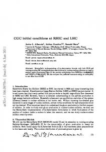
Fig. 1. Photograph of the facility

NASA/TM—2004-212392

8

Fig. 3. Time averaged density profiles from indicated axial stations and Jet Mach numbers. + +: experimental data; _____ : probe-volume-averaged profile (equation 8); - - - - : corrected profile without averaging effect.

Fig. 4. Sketch to explain the effect of a long probe length on measured shear layer profile.

NASA/TM—2004-212392

Fig. 5. Momentum thickness variation in indicated Mach number jets. Symbol: experimental data; solid line: least square linear fit (described in legend). 9

Fig. 7. Momentum thickness variation at the exit of a convergent nozzle with increasing plume Mach number.

Fig. 6. Time average velocity profiles measured using a hot-wire probe. + +: Experimental data; - - - -: Model profile with the same half width b as of Figs. 3(a) & 3(b)

Fig. 8. Density fluctuation spectra from Mach 1.8 jet along r/D = 0.48 and at indicated axial positions. Successive plots are shifted by a multiplication factor of 2.

NASA/TM—2004-212392

10

NASA/TM—2004-212392

11

Fig. 9. Growth of indicated Strouhal frequency fluctuations in 195 Hz. wide frequency bands from three different Mach number jets.

Form Approved OMB No. 0704-0188

REPORT DOCUMENTATION PAGE

Public reporting burden for this collection of information is estimated to average 1 hour per response, including the time for reviewing instructions, searching existing data sources, gathering and maintaining the data needed, and completing and reviewing the collection of information. Send comments regarding this burden estimate or any other aspect of this collection of information, including suggestions for reducing this burden, to Washington Headquarters Services, Directorate for Information Operations and Reports, 1215 Jefferson Davis Highway, Suite 1204, Arlington, VA 22202-4302, and to the Office of Management and Budget, Paperwork Reduction Project (0704-0188), Washington, DC 20503.

1. AGENCY USE ONLY (Leave blank)

2. REPORT DATE

3. REPORT TYPE AND DATES COVERED

Technical Memorandum

May 2004 4. TITLE AND SUBTITLE

5. FUNDING NUMBERS

Measurement of Initial Conditions at Nozzle Exit of High Speed Jets WBS–22–714–08–14

6. AUTHOR(S)

J. Panda, K.B.M.Q. Zaman, and R.G. Seasholtz 7. PERFORMING ORGANIZATION NAME(S) AND ADDRESS(ES)

8. PERFORMING ORGANIZATION REPORT NUMBER

National Aeronautics and Space Administration John H. Glenn Research Center at Lewis Field Cleveland, Ohio 44135 – 3191

E–13969

9. SPONSORING/MONITORING AGENCY NAME(S) AND ADDRESS(ES)

10. SPONSORING/MONITORING AGENCY REPORT NUMBER

National Aeronautics and Space Administration Washington, DC 20546– 0001

NASA TM—2004-212392 AIAA–2001–2143

11. SUPPLEMENTARY NOTES

Prepared for the Seventh Aeroacoustics Conference cosponsored by the American Institute of Aeronautics and Astronautics and the Confederation of European Aerospace Societies, Maastricht, The Netherlands, May 28–30, 2001. J. Panda, Ohio Aerospace Institute, Brook Park, Ohio 44142; K.B.M.Q. Zaman and R.G. Seasholtz, NASA Glenn Research Center. Responsible person, J. Panda, organization code 5860, 216–433–8891. 12b. DISTRIBUTION CODE

12a. DISTRIBUTION/AVAILABILITY STATEMENT

Unclassified - Unlimited Subject Category: 07

Distribution: Nonstandard

Available electronically at http://gltrs.grc.nasa.gov This publication is available from the NASA Center for AeroSpace Information, 301–621–0390. 13. ABSTRACT (Maximum 200 words)

The time averaged and unsteady density fields close to the nozzle exit (0.1 £ x/D £ 2, x: downstream distance, D: jet diameter) of unheated free jets at Mach numbers of 0.95, 1.4, and 1.8 were measured using a molecular Rayleigh scattering based technique. The initial thickness of shear layer and its linear growth rate were determined from timeaveraged density survey and a modeling process, which utilized the Crocco-Busemann equation to relate density profiles to velocity profiles. The model also corrected for the smearing effect caused by a relatively long probe length in the measured density data. The calculated shear layer thickness was further verified from a limited hot-wire measurement. Density fluctuations spectra, measured using a two-Photomultiplier-tube technique, were used to determine evolution of turbulent fluctuations in various Strouhal frequency bands. For this purpose spectra were obtained from a large number of points inside the flow; and at every axial station spectral data from all radial positions were integrated. The radiallyintegrated fluctuation data show an exponential growth with downstream distance and an eventual saturation in all Strouhal frequency bands. The initial level of density fluctuations was calculated by extrapolation to nozzle exit.

14. SUBJECT TERMS

15. NUMBER OF PAGES

17

Jet noise; Turbulence; Rayleigh scattering 17. SECURITY CLASSIFICATION OF REPORT

Unclassified NSN 7540-01-280-5500

18. SECURITY CLASSIFICATION OF THIS PAGE

Unclassified

16. PRICE CODE 19. SECURITY CLASSIFICATION OF ABSTRACT

20. LIMITATION OF ABSTRACT

Unclassified Standard Form 298 (Rev. 2-89) Prescribed by ANSI Std. Z39-18 298-102