Measurement of Pulsewidth via Correlations in ... - Princeton Physics

Measurement of Pulsewidth via Correlations in Intensity Fluctuations M.S. Zolotorev Center for Beam Physics, Lawrence Berkeley National Laboratory, Berkeley, CA 94720

K.T. McDonald Joseph Henry Laboratories, Princeton University, Princeton, NJ 08544 (DRAFT, March 23, 1999, DRAFT)

100% fluctuations in the intensity as a function of frequency, and the itensity spectrum appears noisy. In optics, a source whose intensity is n times that of a unit source, and whose intensity fluctuations have rms magnitude n, is called a “thermal” or “chaotic” source, as first described by Rayleigh [1]. In case of a signal based on n independent samples, one class of fluctuations √ will have size n. The 100% intensity fluctuations that arise here should perhaps be called fluctuations of the fluctuations, as discussed in greater detail in sec. VI. The light from a thermal source, although described as incoherent, still manifests intensity correlations that contain information as to the temporal pulsewidth of the source, which can be extracted with a suitable detector. For a frequency extremely close to ω0 , the phases of the amplitudes from the various electrons of a given pulse are still extremely close to those for radiation at ω0 , and the total amplitude and intensity are still very close to those at ω0 . That is, although the frequency spectrum is subject to 100% fluctuations, there is a correlation length, Γω , in frequency. The size of is the correlation length Γω can be estimated by noting that in going from frequency ω to ω+Γω , the phase difference of radiation from electrons that are the pulsewidth ∆t apart changes by about 180◦ , so that the amplitude for radiation at ω + Γω is no longer well correlated to that at frequency ω. At once, we expect that

Einstein was the first to note that the sky would not be blue without fluctuations in the distribution of the molecules that scatter sunlight. It follows that the intensity of the scattered light fluctuates. These fluctuations are practically undetectable for a large scattering volume such as the atmosphere. However, for a localized source, there result dramatic fluctuations in intensity with a correlation length in frequency that varies inversely with the source size. Measurement of the correlation in intensity fluctuations permits a determination of the pulsewidth in, for example, the synchrotron radiation emitted by a pulse of electrons passing through a magnetic field

I. INTRODUCTION

We conisder a novel method to measure the width, ∆t, of a pulse of relativistic electrons (a beam pulse), via the correlations in the intensity fluctuations of radiation emitted when the pulse passes through a magnetic field. Since intensity fluctuations appear to be a kind of noise, this technique is somewhat counterinituitive. The measurement is based on synchrotron radiation, whose spectrum extends up to a maximum angular frequency ωmax À 1/∆t. This behavior indicates that the radiation is not (first-order) coherent. Then, we can examine the frequency spectrum around a central frequency, ω0 À 1/∆t. At this high frequency, we must take into account the phase difference between light emitted by different electrons in the beam pulse. Indeed, if the electrons were arranged on a lattice, the phase differences would result in essentially complete destructive interference, and there would be no signal. But because of fluctuations in the positions of the electrons, a useful signal results. For n electrons, the average intensity at frequency ω0 À 1/∆t is n √times that from a single electron; the rms amplitude is n times that for a single electron. The radiation at such frequencies is incoherent, in contrast to coherent radiation for which the intensity is n2 times that for a single electron. The amplitude of the radiation at a particular frequency could, of course, be positive, or negative, or very close to zero. Thus, if we examine the radiation spectrum over a range of frequencies near ω0 , the amplitudes will √ vary over the range ± n; the intensity will vary between 0 and n (times that due to a single electron). There are

Γω ≈

1 . ∆t

(1)

The correlation length varies inversely with the pulsewidth. This permits a measurement of the pulsewidth by a measurement of the frequency correlation length. Furthermore, the accuracy of the measurement will be greater for a short pulse than for a long one. This scheme was proposed by one of us [2,3], and recently has been confirmed in the laboratory [4]. It has also been considered in [5]. Section II discusses aspects of the measurement by this technique. Sections III-VII present more detailed derivations of the concept, but without adding anything fundamentally new to the short description given above.

1

The shortest pulse that could be measured this way corresponds to Γω ≈ ω0 , i.e., c∆t ≈ λ0 [≈ 1 µm ≈ 3 fs for an optical detector].

II. DISCUSSION

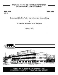
The pulsewidth measurement was demonstrated with the apparatus shown in Fig. 1 [4], which collected spectra such as those shown in Fig. 2. MICROWIGGLER

III. NONRELATIVISTIC DC CURRENT

e MICROBUNCH

The electromagnetic fields of a closed loop of a continuous charge distribution in steady motion with any velocity have no time dependence, and hence, no radiation. However, individual charges moving with velocity v in, for example, a ring of radius r are subject to accelerations v 2 /r (with v ≈ 1 m/s for a copper wire), and would radiate if they were in isolation. How does the radiation come to be suppressed as the charge distribution changes from a discrete collection of n charges to an effectively continuous distribution of a large number of charges? Following J.J. Thomson [6], we note that for a ring of charge, radiation is expected only at harmonics of the fundamental angular frequency ω = v/r. Indeed, the field component at the mth harmonic depends on the strength of the mth multipole of the charge distribution, which depends on the mth power of the positions of the charges. For example, if θ is the azimuthal angle of some electron to the z axis, which is both a diameter of the ring and the line of sight to the observer, then the mth multipole moment depends on cosm θ, which has a leading term of cos mθ = Re(eimθ ). For n particles regularly spaced around a ring that rotates with angular frequency ω, the jth particle has azimuth θj = ωt + 2πj/n, and so the total contribution to the mth moment is proportional to X X eim(ωt+2πj/n) = eimωt e2imπj/n . (3)

IRIS 632 nm SPONTANEOUS EMISSION

SPECTROMETER AND ICCD

FIG. 1. The apparatus used in [4] to measure the pulsewidth of an electron bunch via frequency correlations. The beam energy was 44 MeV, and each pulse contained about 109 electrons. Synchrotron radiation was generated in a 50-cm-long wiggler with 0.9-cm period and peak magnetic field of 0.4 T. Visible radiation centered about 620 nm was analyzed in a spectrometer with 0.6-nm resolution.

j

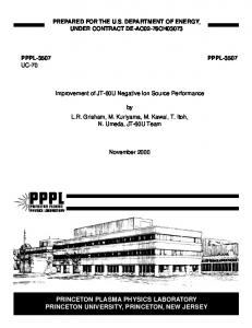
FIG. 2. Single-shot spectra of a portion of the synchrotron radiation from electron pulses measured by another technique to have pulsewidths of 1.5 ps (top) and 4.5 ps (bottom) [4].

j

For large n, this sum is negligible unless the harmonic number m is a multiple of n, in which case the sum is n. That is, for n charges, the lowest contributing multipole moment is of order n. But the radiated power at the nth multipole varies as (v/c)2n , so for nonrelativistic velocities, as in a wire, the radiation is heavily suppressed. A more detailed treatment [6] shows that the radiated power at the nth harmonic is proportional to (nv/c)2n /(n!)2 , which reduces to (v/c)2n with the aid of Stirling’s approximation. Recall that the use of a multipole expansion is a systematic way of treating interference effects between charges at different places within a localized source. See also problems 14.23 and 14.24 of [7], or problem 12.53 of [9].

The intensity spectrum looks something like a random ‘comb’, with ‘teeth’ whose average height is n times that due to a single electron, and whose width in frequency is Γω = 1/∆t. As seen in Fig. 2, the teeth are indeed wider for the shorter electron beam pulse. If one could not resolve the teeth, the spectrum would, of course, appear to be smooth. This is what happens when we look at the sky. The strength of the scattered light depends on the density of the molecules (and not on the square of the density). But, because the atmosphere is thick, the frequency correlation length is extremely short – much less than the spectral resolution of our eyes. Hence, we have no everyday experience of the ‘frequency comb’. Some remarks about measurements: c ω0 ω0 c = ≈ λ0 . (2) c∆t ≈ Γω ω0 Γω Γω

IV. RELATIVISTIC DC CURRENT AND LONG PULSES

Instead of nonrelativistic currents in wires, consider relativistic electron beams moving in a magnetic field. 2

and

There is no kinematic suppression of high multipole radiation here – synchrotron p radiation peaks at the γ 3 harmonic [7,8], where γ = 1/ 1 − (v/c)2 . Hence the nonrelativistic argument of sec. III does not suffice here. Rather, we note that in the relativistic case, the fundamental frequency has wavelength of order of the ring circumference, and higher harmonics have wavelengths shorter than this. Over a distance of one wavelength at a high harmonic, the arc of the ring is essentially a straight line. The interference that suppress the radiation in the relativistic case must apply to sources that are effectively straight lines. Since the effect of a line source is easy to calculate, and corresponds to a short bunch of electrons in the laboratory, we only treat line sources from now on. In the remainder of this section, we demonstrate the expected result that a smooth distribution of charge moving along a line does not radiate at wavelengths small compared to the characteristic length (bunch length) of the distribution. At wavelengths larger than the bunch length, coherent radiation is observed from n charges with intensity n2 times that from a single charge. Consider a charged particle moving with v ≈ c primarily along the z axis. The particle emits radiation that is detected, for simplicity, in the forward direction. The observer is at z = r. The amplitude of the detected radiation from the single charge (emitted when it was at z) is written as Z A = dωa(ω, z)ei[k(r−z)−ωt] , (4)

A(ω)e−iωt .

(8)

A. Continuum Approximation

We replace the sum over j by an integral over z, with ρ(z) describing the effective density of the charges. That is, Z Z A ≈ dzρ(z) dωa(ω)ei[k(r−z)−ωt] Z Z = dωa(ω)ei[kr−ωt] dzρ(z)e−ikz (9) Z = dωa(ω)ρ(ω)ei[kr−ωt] , where ρ(ω = kc) is the Fourier transform of the charge distribution. In the following, we will generally normalize the radiation to that of a single electron. Then it suffices to note that the Fourier components of the field amplitude and of the pulse energy obey A(ω) ∝ ρ(ω) and U (ω) ∝ |ρ(ω)|2 , respectively. B. Uniform Bunch

For example, consider a uniform charge distribution extending from z = 0 to l. Then ρ(z) = n/l on this interval, and Z l n sin kl/2 ρ(ω) = dz e−ikz = ne−ikl/2 . (10) l kl/2 0

where a(ω, z) describes the frequency spectrum of the radiation. The dependence of a on z reflects the details of the radiation process. We do not wish to emphasize those details here, and will ignore the dependence of a on z. This is justified, for example, by supposing that the beam passes through a short region of nearly uniform transverse magnetic field, resulting in a pulse of synchrotron radiation. We next consider a bunch of n charges, which are at positions zj , j = 1, ..., n, at the relevant time of emission. Then n Z X A= dωa(ω)ei[k(r−zj )−ωt] . (5)

This is big only for kl < 1, in which case ρ(ω) ≈ n, and the observer detects coherent radiation from an effective charge of size n. But for wavelengths shorter than the bunch length, the radiation is heavily suppressed (by destructive interference). We learn more by considering the pulse energy, which in a narrow frequency interval will be proportional to |ρ(ω)|2 . Namely, µ ¶2 2n 2 |ρ(ω)| ≈ sin2 kl/2. (11) kl

j=1

The sine varies rapidly between 0 and 1 for small changes in frequency, so we replace it by its average, 1/2. (This corresponds to averaging over uniform charge distributions of lengths near l, but which vary in length by more than a wavelength.) Then, ³ n ´2 ® ­ . (12) |ρ(ω)|2 ≈ 2 kl At high frequencies the radiation falls of as 1/ω 2 , i.e., rather slowly. This is a result of the assumption of a sharp edge to the charge density distribution, which enhances the high-frequency end of the spectrum.

The instantaneous power of the radiation at the observer is proportional to |A|2 . A radiation detector typically integrates the intensity over time to observe the total pulse energy U . The detector may contain a spectrometer that analyzes the pulse energy according to Z U = U (ω)dω, (6) where U (ω) ∝ |A(ω)|2 ,

Z A=

(7) 3

ρ(ω) =

C. Gaussian Bunch

X

nj e−ikzj =

X

j

We also consider a Gaussian distribution of n charges, with rms length σ: ρ(z) = √

2 2 n e−z /2σ . 2πσ

ρ(ω) =

dz √

2 2 2 n e−z /2σ e−ikz = ne−(kσ) /2 . 2πσ

(13)

(14)

This is exponentially suppressed once kσ > 1, showing that a smoothly varying charge distribution results in extremely small radiation as frequencies large compared to the reciprocal of the pulsewidth. V. FLUCTUATIONS

j

where, X

Nj = n,

hδnj i = 0,

The term hAi, which is due to the average charge distribution, is effectively zero for frequencies large compared to 1/∆t. Since the fluctuations, δnj , average to zero, the term hBi is also negligible. All that remains is hCi: ¯2 + *¯¯ ¯ ¯X ¯ −ikzj ¯ ¯ hCi = ¯ δnj e ¯ ¯ j ¯ X X = (δnj )2 + δnj δnl e−ik(zj −zl ) . (19) j

j6=l

The second term of this is zero on average, while ­ ® (δnj )2 = Nj , so X ­ ® |ρ(ω)|2 = hCi = Nj = n, (20) j

for ω À 1/∆t. This is the famous result that the combined intensity of n sources (scattering centers in the blue sky example) is, on average, only n times that of a single source if the sources have a random distribution, and the wavelength is small compared to the source size. This behavior is labelled “thermal”, although no temperature need be invoked to describe it. Therefore, the label “chaotic” is also used sometimes. ­ ® Of course, the result that |ρ(ω)|2 = n is only true on average, and we should also consider the fluctuations about the mean.

(15)

­ ® (δnj )2 = Nj .

l

¯2 + *¯¯ ¯ ¯ ¯X −ikzj ¯ ¯ ≡ hAi + hBi + hCi. δnj e + ¯ ¯ ¯ ¯ j

We now consider the effect of fluctuations in the distribution of the electrons within the beam pulse. The following argument derives from the famous extensions of Smoluchowski [10] and Einstein [11] of of Rayleigh’s treatment of the blue sky [13]. Smoluchowski noted that density fluctuations in the atmosphere lead to a scattered intensity proportional to the number of molecules. Apparently, he initially thought this was an additional contribution to Rayleigh scattering, but Einstein pointed out that interference effects would suppress the scattering in the absence of fluctuations [12]; all Rayleigh scattering is due to density fluctuations. Both Smoluchowski and Einstein noted that density fluctuations play a key role whatever their origin, but their detailed discussion emphasized thermal fluctuations; indeed, in 1910 it was still preferred to use general principles of thermodynamics over models based on molecules. An argument such as that given below, in which temperature is not mentioned, was perhaps first given by Lorentz [14]. The n particles of the bunch are distributed along the z axis. We partition this distribution into intervals, labelled by index j, of length small compared to the wavelength of interest of the radiation, but large enough that the population nj is large compared to one for intervals near the center of the bunch. We label the number of electrons in interval j in the absence of density fluctuations as Nj , and we write the fluctuations about this value as δnj . That is, nj = Nj + δnj ,

(17)

j

The average of the second term is zero, by definition. According to the argument of sec. IV above, the average value of the first term is effectively zero for frequencies large compared to 1/∆t, where ∆t is the electron pulsewidth. That is, the average value is zero for the amplitude Aei(kr−ωt) for the component at frequency ω of a pulse of radiation from n charges. The average is taken over many such pulses. To calculate the rms (root-mean square) value of the amplitude, we consider ¯2 + *¯¯ ¯ X ¯ ¯ ­ ® −ikzj ¯ 2 ¯ Nj e |ρ(ω)| = ¯ ¯ ¯ ¯ j + * X X (18) +2Re  Nj e−ikzj δnl eikzl 

Then, Z

(Nj + δnj )e−ikzj .

(16)

VI. FLUCTUATIONS OF THE FLUCTUATIONS

j

Then, the Fourier transform of the density distribution is

It was noted by Ornstein and Zernike [15] that the arguments of Smoluchowski and Einstein are not suffi4

­ ® = (A + B + C)2 − n2 ­ ® ­ ® ­ ® = A2 + B 2 + C 2

cient in the case where the fluctuations are large, such as near a critical point. That is, Smoluchowski and Einstein did not really explain critical opalescence, but rather the more ordinary case of Rayleigh scattering away from a critical point. When what we call the fluctuations of the fluctuations are important, further analysis is needed based on the concept of correlation functions, first introduced by Ornstein and Zernike. For a general discussion, see [16]. In the example of a narrow pulse of electrons, a phase transition is not possible. However, the concept of a correlation length is highly relevant. This section discusses the variations in the intensity of the radiation at a particular frequency, and the following section takes up the issue of intensity correlations. The intensity is the square of the amplitude, so if the average intensity is n times that of a single √ source, the average amplitude (electric field) must be n times that of a single source. The random phases of the fields from the n sources lead to vector sum of the amplitudes that is a kind of random walk (in amplitude space at a given time) in which the √ total field has a random phase, and rms magnitude n times that of a single source. We note that the average amplitude in this case is zero, and so the intensity has a statistical distribution with zero as the most probable value, and mean n times that due to a single electron. The intensity probability distribution has the exponential form P (|ρ(ω)|2 ) ∝ e−|ρ(ω)|

2

/n

,

(22)

+2Re(hAB ? i + hAC ? i + hBC ? i) − n2 ­ 2® = C − n2 , recalling facts from sec. V. Now, 2 + * X X ­ 2® C =  (δnj )2 + δnj δnl e−ik(zj −zl )  j

j6=l

2 + * X =  (δnj )2 

(23)

j

+2

* X

2

(δnj )

j

+

* X

X

+ δnl δnm e

−ik(zl −zm )

l6=m −ik(zj −zl )

δnj δnl e

j6=l

X

+ δnp δnq e

ik(zp −zq )

.

p6=q

The first term averages to n2 , the second term averages to zero, and the third term averages to zero, except when j = p and l = q (or j = q and l = p). Hence, + * D£ X ¤2 E ­ 2 ® 2 2 2 2 |ρ(ω)| − n = C −n =2 (δnj ) (δnl ) =2

(21)

X

j6=l

Nj Nl .

(24)

j6=l

whose first and second moments are n and 2n2 , respectively, and therefore whose rms spread is n. That is, the intensity fluctuations have the same magnitude as the average intensity; we observe 100% fluctuations at any particular frequency. As an aside, we note that such 100% fluctuations would not occur if the radiation from the individual electrons had amplitudes all of one sign, i.e., if the radiation were unipolar. However, a bounded source cannot emit unipolar electromagnetic radiation [17]. Any real source of electromagnetic radiation produces waves with both positive and negative amplitudes. The existence of 100% intensity fluctuation is possibly counterintuitive in terms of the common argument that a statistical quantity √ based on n samples will have fluctuations of order n. Indeed, the starting point of the discussion in sec. V was that the fluctuations δnj about pthe mean number Nj of electrons in cell j have rms size Nj . Yet, the consequent intensity fluctuations are 100%. It may be helpful to supplement the picture of the random walk of amplitudes with a detailed evaluation of the fluctuations in |ρ(ω)|2 about its average value of n using the notation of sec. V. This approach is useful also in calculating the correlation function in the following section. D£ ® ¤2 E ­ = |ρ(ω)|4 − n2 |ρ(ω)|2 − n

For example, if the n particles were uniformly distributed over m intervals, then Nj = n/m, and D£ ³ n ´2 m(m + 1) ¤2 E |ρ(ω)|2 − n =2 ≈ n2 . m 2

(25)

Thus, the rms fluctuations in |ρ(ω)|2 have size n, which is equal to the average of |ρ(ω)|2 itself! The intensity fluctuations are 100% at any particular frequency. When we look at a cloud-free sky on a sunny day, it is blue, not black and blue! Why don’t we have any everyday experience of the 100% intensity fluctuations? The answer is to be found by considering the intensity at closely neighboring frequencies. VII. FREQUENCY CORRELATIONS

While the distribution of charges is said to be random, the relative positions of the charges are fixed during any particular pulse. The interference among the radiation from the n charges of a particular pulse depends on the phase differences arising from the fixed, but random, spatial distribution of the charges. Of course, the phase differences also depend on the frequency being observed. For a small change in frequency, there is only a small change in the phase differences in a particular pulse. 5

+  X X 0  (δnp )2 + δnp δnq eik (zj −zl ) 

Hence, we expect a strong correlation in the amplitude of the radiation for closely neighboring frequencies. For a pulse of characteristic length l, the correlation will persist from a given frequency ω to frequency ω 0 such that, roughly, the phase difference in the radiation from electrons separated by distance l = c∆t is different by 180◦ at frequencies ω and ω 0 . A large amplitude at frequency ω would then correspond to essentially zero amplitude at frequency ω 0 , etc. The correlation persists over wave numbers such that ∆kl = ∆ω∆t ≈ 1, which translates into a frequency correlation length of 1 . Γω ≈ ∆t

p

=

j

p6=q 2

(δnj )

X

+ 2

(δnl )

(29)

l

*

³ ´ X X 0 +2 (δnj )2 δnp δnq eik(zj −zl ) + eik (zj −zl ) *

j

p6=q

X 0 + (δnj )2 (δnl )2 ei(k−k )(zj −zl ) *

(26)

+

+

+

j6=l

+

X

0

δnj δnl δnp δnq e−ik(zj −zl ) e−ik (zp −zq )

j6=l6=p6=q

On the other hand, for frequencies that differ by a few correlation lengths, it is not improbable that the intensities have similar values, but with one or more dips to near zero at intermediate frequencies. The intensity spectrum appears to consist of spikes of width Γω , with average separation also Γω . The heights of the spikes follow the exponential distribution (21) with mean n times that of the radiation from a single electron and rms variation equal to the mean. This spectral structure can only be observed by a detector with a frequency bandwidth larger than Γω . Otherwise, the signal is averaged over the fluctuations, which latter are then not detectable. For example, the frequency correlation length of the blue sky is much less than the spectral resolution of our eyes, so we are unaware of the 100% intensity fluctuations. A formal measure of the intensity correlation is the correlation function:

2

=n +

X

0

Nj Nl ei(k−k )(zj −zl ) .

j6=l

Writing k − k 0 = ∆k, the correlation function (27) is X Γ(ω, ω 0 ) = Nj Nl ei∆k(zj −zl ) j6=l

Z ≈

Z i∆kz

dzhρ(z)ie

0

dz 0 hρ(z 0 )ie−i∆kz .

(30)

We consider the example of n charges distributed uniformly over a bunch of length l = c∆t, for which hρ(z)i = n/l. Then, Γ(ω, ω 0 ) = n2

2 sin2 ∆kl/2 2 sin ∆ω∆t/2 = n , (∆kl/2)2 (∆ω∆t/2)2

(31)

where ∆ω = ω − ω 0 . As expected, Γ is large only for ∆kl = ∆ω∆t < 1. Thus, the pulsewidth ∆t can be extracted from a measurement of the frequency spectrum of the pulse, by constructing the correlation function Γ(ω, ω 0 ) from the observed data, and fitting it to the above form. Similarly, for a Gaussian bunch of particles with ρ(z) = 2 2 √ ne−z /2σ / 2πσ, the frequency correlation function is

Γ(ω, ω 0 ) = hU (ω)U (ω 0 )i − hU (ω)ihU (ω 0 )i ­ ® ­ ®­ ® ∝ |ρ(ω)|2 |ρ(ω 0 )|2 − |ρ(ω)|2 |ρ(ω 0 )|2 . (27) This is expected to be big for ω = ω 0 , and near zero for ∆ω greater than the correlation length Γω . The correlation function Γ also arises when considering fluctuations in the total pulse energy: ¿Z Z À ­ 2® 2 2 0 2 0 U − hU i ∝ |ρ(ω)| |ρ(ω )| dωdω ¿Z À¿Z À 2 0 2 0 − |ρ(ω)| dω |ρ(ω )| dω (28) Z Z = Γ(ω, ω 0 )dωdω 0 .

2

Γ(ω, ω 0 ) = n2 e−(∆k)

σ2

2

= n2 e−(∆ω)

σt2

.

(32)

Again, the frequency correlation length is ∆ω ≈ 1/σt ≈ 1/∆t. For completeness, weRcalculate the fluctuations in the R total pulse energy U ∝ |ρ(ω)|2 dω = n dω. Z Z ­ ® 2 2 σU = U 2 − hU i ∝ Γ(ω, ω 0 )dωdω 0 Z Z Z sin2 ∆ω∆t/2 n2 dωdω 0 ≈ dω (33) = n2 (∆ω∆t/2)2 ∆t

To evaluate the correlation function Γ, we use the notation of (18) that |ρ(ω)|2 = Aω + Bω + Cω . Then, ­ ® |ρ(ω)|2 |ρ(ω 0 )|2 = h(Aω + Bω + Cω )(Aω0 + Bω0 + Cω0 )i = hCω Cω0 i  * X X =  (δnj )2 + δnj δnl e−ik(zj −zl )  j

* X

That is, 2 σU 1 1 R = . U2 ∆t dω

j6=l

6

(34)

R The integral dω is roughly the total bandwidth of the radiation. Since the premise of the entire analysis was that the total bandwidth be much larger than 1/∆t, we conclude that the pulse energy fluctuations are small, but we cannot be much more precise than this without further assumptions.

Only 10 pulses would be needed for a 1% measurement. The arguments in this section have presupposed that there is enough light detected in each frequency bin that a classical analysis holds. See sec. XI for a discussion of quantum effects. IX. EFFECT OF LIMITED BANDWIDTH

VIII. MEASUREMENT ACCURACY X. TRANSVERSE EFFECTS

We make a simplified estimate of the accuracy of the measurement of the pulsewidth ∆t. The measurement takes place using light near the central frequency ω0 . A spectrometer is used to analyze the radiation into Nω intervals (bins) of width ∆ω0 , where that latter is taken to be the resolution of the spectrometer. The number of intervals NΓ corresponding to one frequency correlation length, Γω ≈ 1/∆t, is then NΓ = Γω /∆ω0 ≈ 1/∆t∆ω0 . Of course, this technique does not work unless the frequency correlation length can be resolved by the spectrometer, i.e., unless NΓ ≥ 1. Hence, the technique applies to short pulses, but is inappropriate for long ones! For very short pulses, the required number of spectrometer bins NΓ to contain one frequency correlation length may exceed the available number NΓ , and a measurement cannot be made. The range of pulsewidths that can be analyzed is 1 1 < ∆t < , Nω ∆ω0 ∆ω0

In the preceding analysis we have used the simplifying approximation that the electron bunch is a line source. Of course, this cannot be true in practice, so we must consider whether there is any important effect due to the finite transverse extent of the bunch. Indeed, if the transverse diameter d of the bunch is too large there will be significant additional phase differences between radiation from electrons at different transverse positions, and the phase information as to the longitudinal structure of the bunch will be diluted. Such concerns were first studied extensively by van Cittert [18] and Zernike [19], who used the term “transversely coherent” to describe a source for which phase differences from points at different transverse coordinates are negligible. In brief, if light of wavelength λ from a source of diameter d is processed through an aperture of diameter D at distance S from the source, then the additional phase differences are negligible if the angular size of the aperture, D/S, is less that the diffraction angle, λ/d, associated with light of wavelength λ emitted by a source of diameter d. The largest aperture for which this is true is called the transverse coherence length, Dcoh , at distance S from the source, for which

(35)

always assuming that the pulsewidth is large compared to 1/ω0 . If the spectrometer had exactly Nω = NΓ frequency bins, and if only a single pulse were analyzed, a primitive measurement of the pulsewidth could be made, but the uncertainty would be essentially 100%. For a spectrometer with a larger value of Nω , but still for only a single pulse, we would obtain approximately Nω /NΓ separate measurements of the pulsewidth. Then, in a total of NP pulses we obtain roughly NP Nω /NΓ measurements, and the relative accuracy of the pulsewidth measurement is given by s r r σ∆t NΓ ∆t∆ω0 ∆t(∆ω0 /ω0 )ω0 ≈ ≈ = , (36) ∆t NP Nω NP Nω NP Nω

λ Dcoh ≈ S . d

(38)

For the present example, it suffices to suppose that the wiggler parameters were chosen so that the optical radiation was synchrotron radiation (rather than undulator radiation) near the critical frequency ωC ≈ γ 3 c/R, where R is the radius of curvature of the electrons’ trajectory in the wiggler. Then, as discussed in ref. [8], the radiation has a characteristic angular spread θ0 ≈ 1/γ, and is exponentially suppressed at larger angles. Therefore, in the present application, most of the light will be collected by an aperture that obeys D/S = θ0 . We desire that the physical aperture D be equal to the transverse coherence length Dcoh to avoid loss of longitudinal phase information. Then, eq. (38) indicates that the electron bunch should have transverse diameter

where we have introduced the resolution of the spectrometer, ∆ω0 /ω0 . Within the domain (35) where measurements are possible, the results are more accurate for shorter pulses! For example, consider a spectrometer with ∆ω0 /ω0 ≈ 10−4 operating with green light (ω0 ≈ 4 × 1015 /s). With a detector having ≈ 400 channels (each matched to ∆ω0 ), the accuracy of measurement of a single pulse of width ∆t = 1 ps would be r 1 10−12 · 4 × 1015 · 10−4 σ∆t ≈ ≈ . (37) ∆t 400 30

d< ∼

λ θ0

(39)

Also, if the electrons in the bunch have an angular spread θ that is larger than the characteristic radiation angle θ0 , not all of the radiation is useful. The product 7

electrons, which have magnitude hnω i according p to (21), there are quantum fluctuations of magnitude hnω i. So long as hnω i > 1, classical considerations dominate. In general, the two types of fluctuations combine in quadrature to yield ­ ® 2 (δnω )2 = hnω i + hnω i = hnω i(hnω i + 1). (42)

of the transverse size d and angular spread θ is called the transverse emittance ² of the source. We see from (39) that the transverse emittance should obey ²< ∼ λ.

(40)

Electrons beams that satisfy (40) are said to be of optical quality. Common units for emittance are mm-mrad = 10−6 m-rad. Since optical wavelengths have λ ≈ 10−6 m, an optical-quality electron beam must have transverse emittance less than about 1 mm-mrad. An interesting variant of the above issues is the question: what is the apparent transverse size of the source of synchrotron radiation from an electron beam of very small transverse emittance? For example, consider radiation from a single electron, whose transverse position can be known to a Compton wavelength (≈ 10−11 cm). However, the apparent source size as determined from its synchrotron radiation is much larger. Indeed, the laws of diffraction require that a radiation pattern with characteristic angle θ0 have an apparent source size that we write as dcoh

λ ≈ γλ, ≈ θ0

This expression is a manifestation of Bose-Einstein statistics. It appears to have been first applied to the context of photodetectors by Purcell [20] in a commentary on the Brown-Twiss effect [21–23]. The present considerations of the extraction of information as to pulse size from intensity correlations in frequency can be considered a variant the Brown-Twiss effect in which intensity correlation in time or space give a measure of source size. For an overview of this subject, see [24]. The probability distribution for which (42) is the variance was shown by Mandel [25,26] to be n

P (nω ) =

hnω i ω , (1 + hnω i)nω +1

(43)

which a form of the Bose-Einstein distribution. The usual caveat to eqs. (42-43) is that they apply only if the photodetector response time is short compared to the coherence time 1/∆ω0 of the light being analyzed. In the present case, this requirement is met by having a source that emits a pulse of radiation with ∆t < 1/∆ω0 , rather than by having a fast photodetector. However, for the application of pulsewidth measurement, we remain most interested in the strongsignal regime in which classical considerations dominate. Therefore, we desire a clear indicator of when we are in the classical regime.

(41)

where the second form holds for synchrotron radiation near the critical frequency. That is, the apparent transverse source size for synchrotron radiation from a single electron just saturates the van-Cittert-Zernike criterion (39) for transverse coherence. In ref. [8], it is shown that this conclusion can be reached from another another perspective. XI. QUANTUM EFFECTS

B. The Photon Degeneracy Parameter

The preceding analysis has been entirely classical so far as the electromagnetic waves are concerned. The n charges have, of course, been assumed to have discrete, identical values. In a quantum view, electromagnetic radiation can be described in terms of photons, and the pulse energy ∆U = Uω ∆ω observed in a frequency interval ∆ω corresponds, on average, to nω = ∆U/¯hω photons. Quantum optics is concerned with quantum effects on the detection of these photons, while accelerator physics is more concerned with quantum effects on electron beams that radiate photons. Here, we touch on a few relevant aspects of quantum optics, and conclude with some brief remarks on quantum fluctuations in electron storage rings.

The distinction between classical and quantum regimes of optics is usefully characterized by the photon degeneracy parameter δω , which is the number of photons per unit cell of size h3 of 6-dimensional phase volume. The degeneracy parameter is perhaps more memorably stated as the number of photons per mode, as introduced by Einstein [27]. It relevance to optical correlation phenomena was first noted by Brown and Twiss [22]. When the source area is larger than that of the detector aperture, the degeneracy parameter for frequency interval ∆ω can be restated as the number of photons per coherence volume Vcoh , where the latter is the product of the square of the transverse coherence length Dcoh of (38) and c times the coherence time [28]. In this case,

A. Bose-Einstein Statistics

Vcoh =

What are the fluctuations δnω in the number nω of observed photons? In addition to the classical fluctuations in the intensity of synchrotron radiation from a bunch of

2 cDcoh ∆ω

(Large source).

(44)

However, if the source area is much smaller than that of the detector aperture, as holds for studies of synchrotron radiation, the transverse phase volume at the 8

detector contains strong rPr correlations, where r is the radial coordinate on the detector surface. In this case, it is more appropriate to define the coherence volume in terms of the transverse coherence length dcoh at the source (eq. (41) for synchrotron radiation), rather than at the detector: Vcoh =

cd2coh ∆ω

(Small source).

where k is Boltzmann’s constant. For high temperatures, δω ≈ kT /¯hω. Thus, for the experiment in which δω ≈ 104 and h ¯ ω ≈ 2 eV, the effective temperature is kT ≈ 2 × 104 eV, or T ≈ 2.5 × 107 K. In this sense, synchrotron radiation provides a very hot source. It is interesting to note that sunlight has a degeneracy parameter δω ≈ 0.02, corresponding to black-body radiation at T ≈ 6, 000K.

(45)

To verify this, note that for a transversely small source, the angular spread θ of the light is of order θ = λ/dcoh . The transverse momentum of the light then has spread ∆P⊥ ≈ P θ ≈ (h/λ)(λ/dcoh ) = h/dcoh , so dcoh∆P⊥ ≈ h. The longitudinal momentum spread within a frequency interval ∆ω0 is ∆Pk = ¯h∆ω/c, so ∆Pk c/∆ω ≈ h. Altogether, ∆P⊥2 ∆Pk Vcoh ≈ (∆P⊥ dcoh )2 ∆Pk

c ≈ h3 , ∆ω

C. Quantum Fluctuations in Electron Storage Rings

When one considers the effect of quantum fluctuations on electrons circulating in a storage ring, a different and much lower effective temperature than that deduced from (50) is relevant. Damping, Hawking-Unruh.....

(46)

[1] Lord Rayleigh, On the Character of the Complete Radiation at a Given Temperature, Phil. Mag. 27, 460-469 (1889); also in Scientific Papers, Vol. 3 (Cambridge U. Press, Cambridge, 1899), pp. 268-276; Phases at Random, sec. 42a of The Theory of Sound, 2nd ed. (1894), reprinted by (Dover, New York, 1945), pp. 35-42. [2] M.S. Zolotorev and G.V. Stupakov, Fluctuational Interferometry for Measurement of Short Pulses of Incoherent Radiation, SLAC-PUB-7132 (March 1996); http://www.slac.stanford.edu/pubs/slacpubs/7000/slacpub-7132.pdf [3] M.S. Zolotorev and G.V. Stupakov, Spectral Fluctuations of Incoherent Radiation and Measurement of Longitudinal Bunch Profile, Proc. PAC97 (Vancouver, B.C., May, 1997), pp. 2180-82; http://www.triumf.ca/pac97/papers/pdf/5P057.PDF [4] P. Catravas et al., Measurement of electron beam bunchlength and emittance using shot noise-driven fluctuations in incoherent radiation, Phys. Rev. Lett. 82, 5261-5264 (1999). [5] J. Krzywinski et al., A new method for ultrashort electron pulse-shape measurement using synchrotron radiation from a bending magnet, Nucl. Instr. and Meth. A401, 429-441 (1997). [6] J.J. Thomson, The Magnetic Properties of Systems of Corpuscles describing Circular Orbits, Phil. Mag. 6, 673693 (1903). [7] J.D. Jackson, Classical Electrodynamics, 3rd ed., (Wiley, New York, 1999). [8] M.S. Zolotorev and K.T. McDonald, Classical Radiation Processes in the Weizs¨ acker-Williams Approximation, http://puhep1.princeton.edu/mcdonald/accel/weizsacker.ps ˜ [9] V.V. Batygin and I.N. Toptygin, Problems in Electrodynamics, 2nd ed. (Academic Press, London, 1978). [10] M.v. Smoluchowski, Molekular-kinetische Theorie der Opaleszens von Gasen im kritischen Zustande, sowie einiger verwandter Erscheinungen, Ann. d. Phys. 25, 205226 (1908); On Opalescence of Gases in the Critical State, Phil. Mag. 23, 165-173 (1912). [11] A. Einstein, Theorie der Opaleszens von homogenen Fl¨ ussigkeiten und Fl¨ ussigkeitsgemishen in der N¨ ahe des

as desired. To estimate the degeneracy parameter for synchrotron radiation, we note that according to eq. (2) of [8], the photon spectrum from a single electron as observed at a frequency ω ≤ ωc in a detector that subtends solid angle θ02 has the remarkably simple form nω ≈ α

∆ω , ω

(47)

where α = e2 /¯hc ≈ 1/137 is the fine structure constant. The transverse extent of this radiation at the source is just dcoh , as discussed in sec. IX. Its longitudinal extent is c∆t, i.e., the pulsewidth. Hence, the photon number density ρω of synchrotron radiation from Ne electrons as it leaves the source is ρω ≈

Ne α∆ω , ωd2coh c∆t

(48)

and the photon degeneracy number is δω = ρω Vcoh ≈

Ne α λ ≈ Ne α , ω∆t c∆t

(49)

using (45). For example, in the experiment of Catravas et al. [4], Ne ≈ 109 , λ ≈ 600 nm, and ∆t ≈ 2 ps, so the photon degeneracy parameter was δω ≈ 104 . Quantum statistics played very little role in that experiment. The degeneracy parameter allows us to assign an effective temperature to synchrotron radiation, which we noted earlier is an excellent example of what has been called a thermal source. As Einstein showed [27], the degeneracy parameter for blackbody radiation at temperature T is δω =

1 , eh¯ ω/kT − 1

(50)

9

[12]

[13]

[14]

[15]

[16]

[17]

[18]

[19]

[20]

[21]

[22]

[23]

kritischen Zustandes, Ann. d. Phys. 33, 1275-1298 (1910); The Theory of the Opalescence of Homogeneous Fluids and Liquid Mixtures near the Critical State, in The Collected Papers of Albert Einstein (Translations), Vol. 3, by A. Beck (Princeton U. Press, Princeton, 1993), [24] pp. 231-249. M.J. Klein et al., eds., Einstein on Critical Opalescence, [25] in The Collected Papers of Albert Einstein, Vol. 3 (Princeton U. Press, Princeton, 1993), pp. 283-285. Lord Rayleigh, On the Light from the Sky, Its Polarization and Colour, Phil. Mag. 41, 107-120, 274-279 (1871); [26] also in Scientific Papers, Vol. 1 (Cambridge U. Press, Cambridge, 1899), pp. 87-103; On the Transmission of [27] Light Through an Atmosphere Containing Small Par[28] ticles in Suspension, and on the Origin of the Blue of the Sky, Phil. Mag. 48, 375-384 (1899); also, Scientific Papers, Vol. 4 (Cambridge U. Press, Cambridge, 1899), pp. 397-405. H.A. Lorentz, The Scattering of Light by Molecules of a Gas, in Problems of Modern Physics (Ginn, Boston, 1925), pp. 52-65. L.S. Ornstein and F. Zernike, Accidental deviations of density and opalescence at the critical point of a single substance, Proc. Roy. Acad. Amsterdam 17, 793-806 (1914). H.E. Stanley, Introduction to Phase Transitions and Critical Phenomena (Oxford U. Press, New York, 1971), chap. 7. K.-J. Kim, K.T. McDonald, G. Stupakov and M.S. Zolotorev, A Bounder Source Can’t Emit a Unipolar Electromagnetic Wave, http://puhep1.princeton.edu/mcdonald/examples/unipolar.ps ˜ P.H. van Cittert, Die wahrscheinliche Schwingungsverteilung in einer von einer Lichtquelle direkt oder mittels einer Linse beleuchteten Ebene, Physica 1, 201-210 (1934); Kohaerenz-Probleme, 6, 1129-1138 (1939) F. Zernike, The Concept of Degree of Coherence and Its Application to Optical Problems, Physics 5, 785-795 (1938); Diffraction and Optical Image Formation, Proc. Phys. Soc. (London) 61, 158-164 (1948). E.M. Purcell, The Question of Correlation between Photons in Coherent Light Rays, Nature 178, 1449-1450 (1956). R.H. Brown and R.Q. Twiss, A New Type of Interferometer for Use in Radio Astronomy, Phil. Mag. 45, 663682 (1954); Correlation between Photons in Two Coherent Beams of Light, Nature 177, 27-29 (1956); A Test of a New Type of Stellar Interferometer on Sirius, 178, 1046-1048; The Question of Correlation between Photons in Coherent Light Rays, Nature 178, 1447-1448 (1956); The Question of Correlation between Photons in Coherent Light Rays, Nature 179, 1128-1129 (1957); Interferometry of the intensity fluctuations in light II. An experimental test of the theory for partially coherent light, Proc. Roy. Soc. 243, 291-319 (1957); Interferometry of the intensity fluctuations in light I. Basic theory: the correlation between photons in coherent beams of radiation, Proc. Roy. Soc. 242, 300-324 (1957). R.Q. Twiss, A.G. Little and R.H. Brown, Correlation between Photons in Coherent Beams of Light, Detected

10

by a Coincidence Counting Technique, Nature 180, 324326 (1957; R.Q. Twiss and A.G. Little, The Detection of Time-Correlated Photons by a Coincidence Detector, Aust. J. Phys. 12, 77-93 (1959). P.W. Milonni and J.H. Eberly, Lasers (Wiley, New York, 1988), Chap. 15. L. Mandel, Fluctuations of Photon Beams and their Correlations, Proc. Phys. Soc. (London) 72, 1037-1048 (1958); Fluctuations of Photon Beams: The Distribution of the Photo-Electrons, 74, 233-243 (1959). L. Mandel and E. Wolf, Optical coherence and quantum optics (Cambridge U. Press, Cambridge, 1995), Chap. 9. A. Einstein, L. Mandel, Photon Degeneracy in Light from Optical Maser and Other Sources, J. Opt. Soc. 51, 797-798 (1961).