Measurement of quantum devices

Measurement of quantum devices Jarom´ır Fiur´ aˇsek and Zdenˇek Hradil Department of Optics, Palack´ y University, 17. listopadu 50, 772 07 Olomouc, Czech Republic

scribe a diverse variety of the physical processes, such as unitary evolution, damping and decoherence. From the reconstructed superoperator G one may further estimate the Liouville superoperator L, which governs the evolution of density matrix in the black box, ̺˙ = L̺. If the superoperator L exists, then G = exp(Lτ ), where τ is the interaction time, and an inversion of this relation yields L [12,13]. kl The estimation of the elements Gij by means of linear algorithms has been addressed in several papers [10–12]. Provided that mapping between known input and output kl states is given, the unknown parameters Gij may be obtained from (1) using the system of linear equations. This linear reconstruction procedure is simple and straightforward, but it suffers from one significant drawback. The kl elements Gij are estimated as a set of seemingly unrelated kl numbers. However, Gij cannot be arbitrary because the linear mapping G must preserve the positive semidefiniteness and trace of the density matrix. These conditions kl impose bounds on the allowed values of Gij . In this Rapid Communication the superoperator G is reconstructed using maximum–likelihood (Max-Lik). It allows to incorporate naturally all the constrains of quantum theory. Since one can only collect a finite amount of data, the linear mapping cannot be determined exactly. In accordance with the probabilistic interpretation of the quantum theory, the Max-Lik estimation answers the question “Which process is most likely to yield the measured data?”. However, Max–Lik solution is not only an estimation, but represents a genuine quantum measurement associated with a quantum device.

arXiv:quant-ph/0009123v1 29 Sep 2000

Maximum-likelihood estimation is applied to identification of an unknown quantum mechanical process represented by a “black box”. In contrast to linear reconstruction schemes the proposed approach always yields physically sensible results. Its feasibility is demonstrated using the Monte Carlo simulations for the two-level system (single qubit). PACS number(s): 03.65.Bz, 03.67.-a

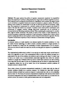
During recent years great attention has been devoted to the measurement of quantum state of various simple quantum mechanical systems. All proposed reconstruction techniques follow the common underlying strategy: A set of measurements is performed on many identically prepared copies of the quantum state which is then estimated from the collected data. Feasible reconstruction schemes were devised for a wide variety of systems including the modes of running electromagnetic field (optical homodyne tomography [1,2] and unbalanced homodyning [3]), cavity electromagnetic field [4,5], motional state of ion in Paul trap [6,7], vibrational state of the molecule [8] and spin [9]. These significant achievements stimulated development of a new remarkable branch of the reconstruction techniques that allow for the experimental determination of the unknown quantum mechanical processes [10–15]. This is of great practical importance, because such a technique may be used, e.g. to evaluate experimentally the performance of the two-bit quantum gate – a building block of quantum computers [10]. The usual set-up considered also in this paper is shown in Fig. 1. Note that a similar experimental configuration can also allow for a complete characterization of quantum measurement [16]. The input state prepared by an experimentalist and characterized by a density matrix ̺in enters the “black box” where it is transformed into the output ̺out . The task for the experimentalist is to retrieve information on the physical process hidden in the black box from the measurements on the output states ̺out . The only assumption taken for granted here is that the mapping ̺out = G̺in is linear, as dictated by the linearity of quantum mechanics, X kl ̺out,ij = Gij ̺in,kl . (1)

Black box

P

ρin

G

ρout

D

Environment FIG. 1. Sketch of experimental set-up for determination of the quantum-mechanical process. The input state ̺in is prepared in the preparator P and enters the black box where it is transformed to the output state ̺out = G̺in which may be entangled with the environment. The detector D measures some observable of the output ̺out .

kl

Here ̺ij = hi|̺|ji are density matrix elements in some complete orthogonal basis of states spanning the Hilbert space on which the density operator ̺ acts. As illustrated in Fig. 1, the system may be entangled with the environment and the transformation G need not preserve purity of the state. The Green superoperator G can de1

Due to its nonlinearity, the Max-Lik estimation is computationally much more expensive task then the linear procedures. This is the prize paid for the physically sound result. Max–Lik estimation has been applied to various problems recently: To the measurements of the quantum phase shift [17], a coupling constant between atom and a cavity electromagnetic field [18], or the parameters of quantum-optical Hamiltonian [19]. Reconstruction of generic quantum state using the Max–Lik estimation and its interpretation as quantum measurement has been proposed in [20]. Subsequent Monte Carlo simulations, performed for the quantum states of electromagnetic field modes and spin [21–23], illustrated a feasibility of this technique. Here we shall demonstrate that the Max-Lik estimation is also suitable for determination of the generic quantum mechanical processes. The sought superoperator G can be found as that one maximizing the likelihood function L[G]. Let us consider n measurements described by positive operator-valued measures (POVM) Π(m) , m = 1, . . . , n. Then L[G] reads L[G] =

n  Y

m=1

=

n Y

m=1



X ijkl

fm

(m) kl (m)  ̺in,kl Πij Gji

(7)

where χjk =

X

cij c∗ik ,

j, k = 0, . . . , N 2 − 1.

(8)

i

Thus χ is positive semidefinite hermitian matrix. This is the desired condition revealing a domain of the allowed kl parameters Gij (or, alternatively, χij ). The matrix χ is parameterized by N 4 real numbers, but the condition (4) imposes N 2 real constraints so that the number of independent parameters reads N 4 − N 2 . When the operator expansion (5) is substituted into Eq. (4), one obtains X m, n = 0, . . . , N − 1, (9) χjk ajk mn = δmn , ˜† ˜ where ajk mn = hm|Ak Aj |ni. The constraints can be also kl expressed in terms of Gij , X

Giikl = δkl .

(10)

i

,

From these N 2 linear constraints one can easily express N 2 real parameters in terms of the remaining N 4 − N 2 ones and thus achieve minimal parameterization. The relation between χ and G can be found by comparing Eqs. (1) and (7),

(2)

where fm is (relative) frequency for detection of Π(m) . Maximum of this function should be found in the domain of physically allowed superoperators G, whose determination is crucial for successful implementation of the Max-Lik estimation. The linear positive map (1) can be conveniently cast into the form which explicitly preserves the positive semidefinitness of the density matrix [11], X Ai ρi A†i . (3) ̺out =

kl Gij

It follows from the condition Tr ̺out = 1 that X † Ai Ai = I,

hi|A˜m |kihl|A†n |jiχmn .

(11)

This formula simplifies considerably if the basis (6) is kl chosen Gij = χiN +k,jN +l . To provide an explicit example, let us consider a two-level system (single qubit). The kl matrix χ can be expressed in terms of Gij as follows, 

01 00 01 00 G01 G01 G00 G00

 10 11 10 11  G00 G00 G01 G01 χ=  G 00 G 01 G 00 G 01  10 10 11 11

(4)

11 10 11 10 G11 G11 G10 G10

i

where I denotes the identity operator. Further we can expand Ai in some complete operator basis A˜j , X (5) cij A˜j . Ai =



  ,  

(12)

kl kl and the constraints (4) yield G11 = δkl − G00 . Thus χ is parameterized by 16 − 4 = 12 real parameters that can be collected in a vector

~ = (G 00 , G 11 , Re G 01 , Im G 01 , Re G 00 , Im G 00 , G 00 00 00 00 01 01 10 10 01 01 11 11 Re G01 , Im G01 , Re G01 , Im G01 , Re G01 , Im G01 ) (13)

j

If we deal with N level system |ii, i = 0, . . . , N − 1, then it is natural to choose the N 2 basis operators as i, j = 0, . . . , N − 1,

=

2 NX −1

m,n=0

i

A˜N i+j = |iihj|,

χjk A˜j ̺in A˜†k ,

jk

ifm h (m) Tr Π(m) ̺out



X

̺out =

lk ∗ kl ) since χ is hermitian. Additional = (Gji Note that Gij kl constraints on Gij follow from the positive semidefiniteness of χ. All four main subdeterminants of the matrix (12) should be non-negative. This can be easily checked for each G where the likelihood function (2) is evaluated. If (12) is not positive semidefinite, then one may simply

(6)

but other constructions are possible. Inserting (5) into (3), we find that

2

On performing the differentiation with respect to A†i , and solving for Ai , we obtain

put L[G] = 0. The maximum of L can be found for example with the help of downhill-simplex algorithm. In case of 2 level system it is sufficient to search for the maximum in the finite volume subspace of 12 dimensional space. Alternatively, one can find the maximum by setting kl to zero all derivatives of L[G] with respect of Gij . It is convenient to work with the log-likelihood function. The constraints (9) must be incorporated by introducing N 2 (complex) Lagrange multipliers λmn = λ∗nm . Thus one arrives at " # X X ∂ mn ln L[G] − λmn Gpp = 0. (14) kl ∂Gij mn p

Ai =

λkl δab =

m

pm

(m) (m) Πba ̺in,kl ,

λ=

Tr λ δab =

(15)

m

(m)

(m)

kp Πba ̺in,kl (λ−1 )ln Gac .

m

m

pm

(m)

(m)

pi Πka Gak ̺in,pj .

pm

Π(m) = I.

Π′(m) =

(24)

fm (m) Π . pm

Moreover, in spite of the fact that the relation used by standard reconstructions pm = fm cannot be fulfilled in general, the analogous relation for the renormalized POVM is identically true X (m) (25) Ai ρin A†i Π′(m) ] ≡ fm . p′m ≡ Tr[

(17)

a,k,l

X fm X

(23)

This is nothing else as the closure relation for renormalized positive valued operator measures

Convenient form of Lagrange multipliers λmn may be found by inserting eq. (17) into (10) λij =

X fm (m) (m) Πba Tr ̺in . p m m

X fm

As follows from Eq. (15) λ is positive definite hermitian matrix. The extremal equation may be rewritten to the form suitable for iterative solution. Multiplying eq. (15) by kp (λ−1 )ln Gac and summing over a, k, l, one gets pm

(22)

Since all the traces are equal to 1, this relation reads in the operator form

i

X fm X

X fm X † (m) Ai Π(m) Ai ̺in , p m i m

P which is equivalent to (18). Notice that Trλ = m fm = 1. The procedure of Max-Lik estimation may be interpreted as a generalized measurement. To show this explicitly, let us put k = l in the relation (15) and add all the elements over k

where we have introduced   X (m) (m) Ai ρin A†i Π(m) ] = Tr Π(m) G̺in . (16) pm = Tr[

np Gbc =

(21)

Next we multiply (21) from the left by operator A†i and sum over i. Taking into account the constraint (4), we find

Eqs. (10) and (14) represent a system of N 4 + N 2 nonlinear equations which must be solved for N 4 elements kl Gij and N 2 Lagrange multipliers λmn . On inserting the explicit expression for the likelihood function (2) into Eq. (14) one obtains, X fm

X fm (m) Π(m) Ai ̺in λ−1 . p m m

(18)

i

a,k,p

This indicates the privileged role of Max-Lik estimation in analogy with the quantum state estimation [20]. Max– Lik estimation represents a genuine quantum measurement. Properties of a quantum black box are determined using the closure relation (24) for a POVM, expectation values of which are the registered data (25). In the rest of the paper we demonstrate the feasibility of our approach by means of Monte Carlo simulations for two-level system (a single qubit). We shall consider spin 1/2 system. The detector D shown in Fig. 1 is SternGerlach apparatus measuring the spin projections along one of three axes x, y, z. We further assume that ̺in is prepared in one of six eigenstates | ↑j i, | ↓j i of the spin projectors (Pauli matrices) σj , j = x, y, z, σj | ↑j i = | ↑j i, and σj | ↓j i = −| ↓j i. We choose the basis |0i = | ↓z i and |1i = | ↑z i. Each of the six input states is prepared

The system of nonlinear equations (17) and (18) for the elements of G can be conveniently solved by repeated iterations. The theory may be formulated in terms of the operators Ai , A†i . It is helpful to define a hermitian operator X λ= λmn |mihn|. (19) mn

The maximum of log-likelihood function can be formally found as the relation ! X † ∂ (20) Ai Ai ] = 0. ln L[{Ai }] − Tr [λ ∂A†i i 3

This work was supported by Grant LN00A015 of the Czech Ministry of Education. This paper is dedicated to the anniversary of 65th birthday of Prof. Jan Peˇrina.

1 0.8 0.6 Gk 0.4 0.2

[1] D.T. Smithey, M. Beck, M.G. Raymer and A. Faridani, Phys. Rev. Lett. 70, 1244 (1993); S. Schiller, G. Breitenbach, S.F. Pereira, T. M¨ uller, and J. Mlynek, Phys. Rev. Lett. 77, 2933 (1996); [2] M. Vasilyev, S-K Choi, P. Kumar, and G. M. D’Ariano, Phys. Rev. Lett. 84, 2354 (2000). [3] S. Wallentowitz and W. Vogel, Phys. Rev. A 53, 4528 (1996); K. Banaszek and K. W´ odkiewicz, Phys. Rev. Lett. 76, 4344 (1996). [4] L.G. Lutterbachand L. Davidovich, Phys. Rev. Lett. 78, 2547 (1997). [5] C.T. Bodendorf, G. Antesberger, M.S. Kim, and H. Walther, Phys. Rev. A 57, 1371 (1998). [6] S. Wallentowitz and W. Vogel, Phys. Rev. Lett. 75, 2932 (1995). [7] D. Leibfried, D.M. Meekhof, B.E. King, C. Monroe, W.M. Itano, and D.J. Wineland, Phys. Rev. Lett. 77, 4281 (1996). [8] T.J. Dunn, I. A. Walmsley, and S. Mukamel, Phys. Rev. Lett. 74, 884 (1995); C. Leichtle, W.P. Schleich, I.Sh. Averbukh, and M. Shapiro, Phys. Rev. Lett. 80, 1418 (1998). [9] R.G. Newton and B. Young, Ann. Phys. New York 49, 393 (1968). [10] J. F. Poyatos, J. I. Cirac, and P. Zoller, Phys. Rev. Lett. 78, 390 (1997). [11] I.L. Chuang and M.A. Nielsen, J. Mod. Opt. 44, 2455 (1997). [12] G. M. D’Ariano and L. Maccone, Phys. Rev. Lett. 80, 5465 (1998); Fortschr. Phys. 46, 837 (1998). [13] V. Buˇzek, Phys. Rev. A 58, 1723 (1998). [14] R. Gutzeit, S. Wallentowitz, and W. Vogel, Phys. Rev. A 61 062105 (2000). [15] A. Luis and L.L. S´ anchez-Soto, Phys. Lett. A 261, 12 (1999). [16] A. Luis and L.L. S´ anchez-Soto, Phys. Rev. Lett. 83, 3573 (1999); [17] Z. Hradil, R. Myˇska, J. Peˇrina, M. Zawisky, Y. Hasegawa, and H. Rauch, Phys. Rev. Lett. 76, 4295 (1996). [18] H. Mabuchi, Quantum semiclass. Opt. 8, 1103 (1996). [19] G. M. D’Ariano, M.G.A. Paris, and M.F Sacchi, Phys. Rev. A 62, 023815 (2000). [20] Z. Hradil, Phys. Rev. A 55, R1561 (1997); Z. Hradil, J. Summhammer, and H. Rauch, Phys. Lett. A 261, 20 (1999). [21] K. Banaszek, Phys. Rev. A 57, 5013 (1998). [22] K. Banaszek, G.M. D’Ariano, M.G.A. Paris, and M. F. Sacchi, Phys. Rev. A 61, 010304(R) (1999). [23] Z. Hradil, J. Summhammer, G. Badurek, and H. Rauch, Phys. Rev. A 62, 014101 (2000).

0 1

2

3

4

5

6

7

8

9 10 11 12

k

FIG. 2. Reconstructed elements of the superoperator G ~ Bars correspond to the plotted in the form of the vector G. Max-Lik estimation (black), linear inversion (grey), and exact values (hollow). Missing hollow bars indicate the zero true values. The superoperator describes the process of damping, Γ|| = 0.5 and Γ⊥ = 0.75, N = 20.

3N times. At the output, one measures N times the spin along each of the three axes x, y, z. The corresponding six projectors read Πj = |jihj|, j =↑x , ↓x , ↑y , ↓y , ↑z , ↓z . Let fjk denote the relative frequency of projections to the state |ki measured for the input state |ji. The likelihood function can be expressed as product of 36 terms, L[G] =

Y   fjk hk| G |jihj| |ki ,

(26)

j,k

where j, k ∈ {↑x, ↓x , ↑y , ↓y , ↑z , ↓z }. In our simulations, the black box of the Fig. 1 corresponds to the damping of ρin , ! 1 − ρin,11 e−Γ|| ρin,01 e−Γ⊥ . (27) ρout = ρin,10 e−Γ⊥ ρin,11 e−Γ|| Here 2Γ⊥ ≥ Γ|| ≥ 0 are transversal and longitudinal decay parameters. The elements of reconstructed superoperator are depicted in the Fig. 2. The solution was obtained by iterations of eqs. (17) and (18). For the total amount of 360 measurements the Max-Lik estimate (black) is very close to the exact values G (hollow). Notice that Max-Lik provides always physically sound result, on the contrary to the linear inversion (grey). Properties of transforming systems are of interest in any physical theory. The developed formalism shows how to describe it as a genuine quantum measurement. Quantum systems consisting of spins, two entangled or three entangled (GHZ) qubits are tractable due to their low dimensionality. Proper and full quantum description of possible transformations of such systems is, however, more advanced, since it is characterized by 12, 240, or even 4032 parameters.

4