Apr 27, 2011 - 7University of Science and Technology of China, Hefei, People's Republic of ... 58Louisiana Tech University, Ruston, Louisiana 71272, USA.
FERMILAB-PUB-11/196-E
arXiv:1104.5194v1 [hep-ex] 27 Apr 2011
Measurement of spin correlation in tt¯ production using a matrix element approach V.M. Abazov,35 B. Abbott,73 B.S. Acharya,29 M. Adams,49 T. Adams,47 G.D. Alexeev,35 G. Alkhazov,39 A. Altona ,61 G. Alverson,60 G.A. Alves,2 L.S. Ancu,34 M. Aoki,48 M. Arov,58 A. Askew,47 B. ˚ Asman,41 65 8 80 13 48 48 O. Atramentov, C. Avila, J. BackusMayes, F. Badaud, L. Bagby, B. Baldin, D.V. Bandurin,47 S. Banerjee,29 E. Barberis,60 P. Baringer,56 J. Barreto,3 J.F. Bartlett,48 U. Bassler,18 V. Bazterra,49 S. Beale,6 A. Bean,56 M. Begalli,3 M. Begel,71 C. Belanger-Champagne,41 L. Bellantoni,48 S.B. Beri,27 G. Bernardi,17 R. Bernhard,22 I. Bertram,42 M. Besan¸con,18 R. Beuselinck,43 V.A. Bezzubov,38 P.C. Bhat,48 V. Bhatnagar,27 G. Blazey,50 S. Blessing,47 K. Bloom,64 A. Boehnlein,48 D. Boline,70 E.E. Boos,37 G. Borissov,42 T. Bose,59 A. Brandt,76 O. Brandt,23 R. Brock,62 G. Brooijmans,68 A. Bross,48 D. Brown,17 J. Brown,17 X.B. Bu,48 M. Buehler,79 V. Buescher,24 V. Bunichev,37 S. Burdinb ,42 T.H. Burnett,80 C.P. Buszello,41 B. Calpas,15 E. Camacho-P´erez,32 M.A. Carrasco-Lizarraga,56 B.C.K. Casey,48 H. Castilla-Valdez,32 S. Chakrabarti,70 D. Chakraborty,50 K.M. Chan,54 A. Chandra,78 G. Chen,56 S. Chevalier-Th´ery,18 D.K. Cho,75 S.W. Cho,31 S. Choi,31 B. Choudhary,28 S. Cihangir,48 D. Claes,64 J. Clutter,56 M. Cooke,48 W.E. Cooper,48 M. Corcoran,78 F. Couderc,18 M.-C. Cousinou,15 A. Croc,18 D. Cutts,75 A. Das,45 G. Davies,43 K. De,76 S.J. de Jong,34 E. De La Cruz-Burelo,32 F. D´eliot,18 M. Demarteau,48 R. Demina,69 D. Denisov,48 S.P. Denisov,38 S. Desai,48 C. Deterre,18 K. DeVaughan,64 H.T. Diehl,48 M. Diesburg,48 A. Dominguez,64 T. Dorland,80 A. Dubey,28 L.V. Dudko,37 D. Duggan,65 A. Duperrin,15 S. Dutt,27 A. Dyshkant,50 M. Eads,64 D. Edmunds,62 J. Ellison,46 V.D. Elvira,48 Y. Enari,17 H. Evans,52 A. Evdokimov,71 V.N. Evdokimov,38 G. Facini,60 T. Ferbel,69 F. Fiedler,24 F. Filthaut,34 W. Fisher,62 H.E. Fisk,48 M. Fortner,50 H. Fox,42 S. Fuess,48 A. Garcia-Bellido,69 V. Gavrilov,36 P. Gay,13 W. Geng,15, 62 D. Gerbaudo,66 C.E. Gerber,49 Y. Gershtein,65 G. Ginther,48, 69 G. Golovanov,35 A. Goussiou,80 P.D. Grannis,70 S. Greder,19 H. Greenlee,48 Z.D. Greenwood,58 E.M. Gregores,4 G. Grenier,20 Ph. Gris,13 J.-F. Grivaz,16 A. Grohsjean,18 S. Gr¨ unendahl,48 M.W. Gr¨ unewald,30 T. Guillemin,16 F. Guo,70 48 73 c 68 47 60 G. Gutierrez, P. Gutierrez, A. Haas , S. Hagopian, J. Haley, L. Han,7 K. Harder,44 A. Harel,69 J.M. Hauptman,55 J. Hays,43 T. Head,44 T. Hebbeker,21 D. Hedin,50 H. Hegab,74 A.P. Heinson,46 U. Heintz,75 C. Hensel,23 I. Heredia-De La Cruz,32 K. Herner,61 G. Heskethd ,44 M.D. Hildreth,54 R. Hirosky,79 T. Hoang,47 J.D. Hobbs,70 B. Hoeneisen,12 M. Hohlfeld,24 Z. Hubacek,10, 18 N. Huske,17 V. Hynek,10 I. Iashvili,67 R. Illingworth,48 A.S. Ito,48 S. Jabeen,75 M. Jaffr´e,16 D. Jamin,15 A. Jayasinghe,73 R. Jesik,43 K. Johns,45 M. Johnson,48 D. Johnston,64 A. Jonckheere,48 P. Jonsson,43 J. Joshi,27 A.W. Jung,48 A. Juste,40 K. Kaadze,57 E. Kajfasz,15 D. Karmanov,37 P.A. Kasper,48 I. Katsanos,64 R. Kehoe,77 S. Kermiche,15 N. Khalatyan,48 A. Khanov,74 A. Kharchilava,67 Y.N. Kharzheev,35 D. Khatidze,75 M.H. Kirby,51 J.M. Kohli,27 A.V. Kozelov,38 J. Kraus,62 S. Kulikov,38 A. Kumar,67 A. Kupco,11 T. Kurˇca,20 V.A. Kuzmin,37 J. Kvita,9 S. Lammers,52 G. Landsberg,75 P. Lebrun,20 H.S. Lee,31 S.W. Lee,55 W.M. Lee,48 J. Lellouch,17 L. Li,46 Q.Z. Li,48 S.M. Lietti,5 J.K. Lim,31 D. Lincoln,48 J. Linnemann,62 V.V. Lipaev,38 R. Lipton,48 Y. Liu,7 Z. Liu,6 A. Lobodenko,39 M. Lokajicek,11 R. Lopes de Sa,70 H.J. Lubatti,80 R. Luna-Garciae ,32 A.L. Lyon,48 A.K.A. Maciel,2 D. Mackin,78 R. Madar,18 R. Maga˜ na-Villalba,32 S. Malik,64 V.L. Malyshev,35 Y. Maravin,57 32 70 J. Mart´ınez-Ortega, R. McCarthy, C.L. McGivern,56 M.M. Meijer,34 A. Melnitchouk,63 D. Menezes,50 P.G. Mercadante,4 M. Merkin,37 A. Meyer,21 J. Meyer,23 F. Miconi,19 N.K. Mondal,29 G.S. Muanza,15 M. Mulhearn,79 E. Nagy,15 M. Naimuddin,28 M. Narain,75 R. Nayyar,28 H.A. Neal,61 J.P. Negret,8 P. Neustroev,39 S.F. Novaes,5 T. Nunnemann,25 G. Obrant,39 J. Orduna,78 N. Osman,15 J. Osta,54 G.J. Otero y Garz´ on,1 46 76 53 75 31 68 c 75 M. Padilla, A. Pal, N. Parashar, V. Parihar, S.K. Park, J. Parsons, R. Partridge , N. Parua,52 A. Patwa,71 B. Penning,48 M. Perfilov,37 K. Peters,44 Y. Peters,44 K. Petridis,44 G. Petrillo,69 P. P´etroff,16 R. Piegaia,1 J. Piper,62 M.-A. Pleier,71 P.L.M. Podesta-Lermaf ,32 V.M. Podstavkov,48 P. Polozov,36 A.V. Popov,38 M. Prewitt,78 D. Price,52 N. Prokopenko,38 S. Protopopescu,71 J. Qian,61 A. Quadt,23 B. Quinn,63 M.S. Rangel,2 K. Ranjan,28 P.N. Ratoff,42 I. Razumov,38 P. Renkel,77 M. Rijssenbeek,70 I. Ripp-Baudot,19 F. Rizatdinova,74 M. Rominsky,48 A. Ross,42 C. Royon,18 P. Rubinov,48 R. Ruchti,54 G. Safronov,36 G. Sajot,14 P. Salcido,50 A. S´ anchez-Hern´ andez,32 M.P. Sanders,25 B. Sanghi,48 A.S. Santos,5 G. Savage,48 L. Sawyer,58 T. Scanlon,43 R.D. Schamberger,70 Y. Scheglov,39 H. Schellman,51 T. Schliephake,26 S. Schlobohm,80 C. Schwanenberger,44 R. Schwienhorst,62 J. Sekaric,56 H. Severini,73 E. Shabalina,23 V. Shary,18 A.A. Shchukin,38 R.K. Shivpuri,28 V. Simak,10 V. Sirotenko,48 P. Skubic,73 P. Slattery,69 D. Smirnov,54 K.J. Smith,67 G.R. Snow,64 J. Snow,72 S. Snyder,71 S. S¨ oldner-Rembold,44 L. Sonnenschein,21 K. Soustruznik,9 J. Stark,14 V. Stolin,36 D.A. Stoyanova,38
2 M. Strauss,73 D. Strom,49 L. Stutte,48 L. Suter,44 P. Svoisky,73 M. Takahashi,44 A. Tanasijczuk,1 W. Taylor,6 M. Titov,18 V.V. Tokmenin,35 Y.-T. Tsai,69 D. Tsybychev,70 B. Tuchming,18 C. Tully,66 L. Uvarov,39 S. Uvarov,39 S. Uzunyan,50 R. Van Kooten,52 W.M. van Leeuwen,33 N. Varelas,49 E.W. Varnes,45 I.A. Vasilyev,38 P. Verdier,20 L.S. Vertogradov,35 M. Verzocchi,48 M. Vesterinen,44 D. Vilanova,18 P. Vokac,10 H.D. Wahl,47 M.H.L.S. Wang,69 J. Warchol,54 G. Watts,80 M. Wayne,54 M. Weberg ,48 L. Welty-Rieger,51 A. White,76 D. Wicke,26 M.R.J. Williams,42 G.W. Wilson,56 M. Wobisch,58 D.R. Wood,60 T.R. Wyatt,44 Y. Xie,48 C. Xu,61 S. Yacoob,51 R. Yamada,48 W.-C. Yang,44 T. Yasuda,48 Y.A. Yatsunenko,35 Z. Ye,48 H. Yin,48 K. Yip,71 S.W. Youn,48 J. Yu,76 S. Zelitch,79 T. Zhao,80 B. Zhou,61 J. Zhu,61 M. Zielinski,69 D. Zieminska,52 and L. Zivkovic75 (The D0 Collaboration∗) 1 Universidad de Buenos Aires, Buenos Aires, Argentina LAFEX, Centro Brasileiro de Pesquisas F´ısicas, Rio de Janeiro, Brazil 3 Universidade do Estado do Rio de Janeiro, Rio de Janeiro, Brazil 4 Universidade Federal do ABC, Santo Andr´e, Brazil 5 Instituto de F´ısica Te´ orica, Universidade Estadual Paulista, S˜ ao Paulo, Brazil 6 Simon Fraser University, Vancouver, British Columbia, and York University, Toronto, Ontario, Canada 7 University of Science and Technology of China, Hefei, People’s Republic of China 8 Universidad de los Andes, Bogot´ a, Colombia 9 Charles University, Faculty of Mathematics and Physics, Center for Particle Physics, Prague, Czech Republic 10 Czech Technical University in Prague, Prague, Czech Republic 11 Center for Particle Physics, Institute of Physics, Academy of Sciences of the Czech Republic, Prague, Czech Republic 12 Universidad San Francisco de Quito, Quito, Ecuador 13 LPC, Universit´e Blaise Pascal, CNRS/IN2P3, Clermont, France 14 LPSC, Universit´e Joseph Fourier Grenoble 1, CNRS/IN2P3, Institut National Polytechnique de Grenoble, Grenoble, France 15 CPPM, Aix-Marseille Universit´e, CNRS/IN2P3, Marseille, France 16 LAL, Universit´e Paris-Sud, CNRS/IN2P3, Orsay, France 17 LPNHE, Universit´es Paris VI and VII, CNRS/IN2P3, Paris, France 18 CEA, Irfu, SPP, Saclay, France 19 IPHC, Universit´e de Strasbourg, CNRS/IN2P3, Strasbourg, France 20 IPNL, Universit´e Lyon 1, CNRS/IN2P3, Villeurbanne, France and Universit´e de Lyon, Lyon, France 21 III. Physikalisches Institut A, RWTH Aachen University, Aachen, Germany 22 Physikalisches Institut, Universit¨ at Freiburg, Freiburg, Germany 23 II. Physikalisches Institut, Georg-August-Universit¨ at G¨ ottingen, G¨ ottingen, Germany 24 Institut f¨ ur Physik, Universit¨ at Mainz, Mainz, Germany 25 Ludwig-Maximilians-Universit¨ at M¨ unchen, M¨ unchen, Germany 26 Fachbereich Physik, Bergische Universit¨ at Wuppertal, Wuppertal, Germany 27 Panjab University, Chandigarh, India 28 Delhi University, Delhi, India 29 Tata Institute of Fundamental Research, Mumbai, India 30 University College Dublin, Dublin, Ireland 31 Korea Detector Laboratory, Korea University, Seoul, Korea 32 CINVESTAV, Mexico City, Mexico 33 FOM-Institute NIKHEF and University of Amsterdam/NIKHEF, Amsterdam, The Netherlands 34 Radboud University Nijmegen/NIKHEF, Nijmegen, The Netherlands 35 Joint Institute for Nuclear Research, Dubna, Russia 36 Institute for Theoretical and Experimental Physics, Moscow, Russia 37 Moscow State University, Moscow, Russia 38 Institute for High Energy Physics, Protvino, Russia 39 Petersburg Nuclear Physics Institute, St. Petersburg, Russia 40 Instituci´ o Catalana de Recerca i Estudis Avan¸cats (ICREA) and Institut de F´ısica d’Altes Energies (IFAE), Barcelona, Spain 41 Stockholm University, Stockholm and Uppsala University, Uppsala, Sweden 42 Lancaster University, Lancaster LA1 4YB, United Kingdom 43 Imperial College London, London SW7 2AZ, United Kingdom 44 The University of Manchester, Manchester M13 9PL, United Kingdom 45 University of Arizona, Tucson, Arizona 85721, USA 46 University of California Riverside, Riverside, California 92521, USA 47 Florida State University, Tallahassee, Florida 32306, USA 48 Fermi National Accelerator Laboratory, Batavia, Illinois 60510, USA 49 University of Illinois at Chicago, Chicago, Illinois 60607, USA 50 Northern Illinois University, DeKalb, Illinois 60115, USA 2
3 51
Northwestern University, Evanston, Illinois 60208, USA Indiana University, Bloomington, Indiana 47405, USA 53 Purdue University Calumet, Hammond, Indiana 46323, USA 54 University of Notre Dame, Notre Dame, Indiana 46556, USA 55 Iowa State University, Ames, Iowa 50011, USA 56 University of Kansas, Lawrence, Kansas 66045, USA 57 Kansas State University, Manhattan, Kansas 66506, USA 58 Louisiana Tech University, Ruston, Louisiana 71272, USA 59 Boston University, Boston, Massachusetts 02215, USA 60 Northeastern University, Boston, Massachusetts 02115, USA 61 University of Michigan, Ann Arbor, Michigan 48109, USA 62 Michigan State University, East Lansing, Michigan 48824, USA 63 University of Mississippi, University, Mississippi 38677, USA 64 University of Nebraska, Lincoln, Nebraska 68588, USA 65 Rutgers University, Piscataway, New Jersey 08855, USA 66 Princeton University, Princeton, New Jersey 08544, USA 67 State University of New York, Buffalo, New York 14260, USA 68 Columbia University, New York, New York 10027, USA 69 University of Rochester, Rochester, New York 14627, USA 70 State University of New York, Stony Brook, New York 11794, USA 71 Brookhaven National Laboratory, Upton, New York 11973, USA 72 Langston University, Langston, Oklahoma 73050, USA 73 University of Oklahoma, Norman, Oklahoma 73019, USA 74 Oklahoma State University, Stillwater, Oklahoma 74078, USA 75 Brown University, Providence, Rhode Island 02912, USA 76 University of Texas, Arlington, Texas 76019, USA 77 Southern Methodist University, Dallas, Texas 75275, USA 78 Rice University, Houston, Texas 77005, USA 79 University of Virginia, Charlottesville, Virginia 22901, USA 80 University of Washington, Seattle, Washington 98195, USA (Dated: April 26, 2011) 52
We determine the fraction of tt¯ events with spin correlation, assuming that the spin of the top quark is either correlated with the spin of the anti-top quark as predicted by the standard model or is uncorrelated. For the first time we use a matrix-element-based approach to study tt¯ spin correlation. We√use tt¯ → W + b W −¯b → ℓ+ νb ℓ− ν¯¯b final states produced in p¯ p collisions at a center of mass energy s = 1.96 TeV, where ℓ denotes an electron or a muon. The data correspond to an integrated luminosity of 5.4 fb−1 and were collected with the D0 detector at the Fermilab Tevatron collider. The result agrees with the standard model prediction. We exclude the hypothesis that the spins of the tt¯ are uncorrelated at the 97.7% C.L. PACS numbers: 14.65.Ha, 12.38.Qk, 13.85.Qk
While top and anti-top quarks are unpolarized in tt¯ production at hadron colliders and their spins cannot be measured directly, their spins are correlated and this correlation can be investigated experimentally [1]. The standard model (SM) of particle physics predicts that top quarks decay before fragmentation [2], which is in agreement with the measured lifetime of the top quark [3]. The information on the spin orientation of top quarks is transferred through weak interaction to the angular distributions of the decay products [4, 5].
visitors from a Augustana College, Sioux Falls, SD, USA, University of Liverpool, Liverpool, UK, c SLAC, Menlo Park, CA, USA, d University College London, London, UK, e Centro de Investigacion en Computacion - IPN, Mexico City, Mexico, f ECFM, Universidad Autonoma de Sinaloa, Culiac´ an, Mexico, and g Universit¨ at Bern, Bern, Switzerland.
∗ with b The
We present a test of the hypothesis that the correlation of the spin of t and t¯ quarks is as expected in the SM as opposed to the hypothesis that they are uncorrelated. The spins could become decorrelated if the spins of the top quarks flip before they decay or if the polarization information is not propagated to all the final state products. This could occur if the top quark decayed into a scalar charged Higgs boson and a b quark (t → H + b) [6– 8]. Recently, the CDF Collaboration has presented a measurement of the tt¯ spin correlation parameter C in semileptonic final states from a differential angular distribution [9]. The spin correlation strength C is defined by d2 σ/d cos θ1 d cos θ2 = σ(1 − C cos θ1 cos θ2 )/4, where σ denotes the cross section, and θ1 and θ2 are the angles between the direction of flight of the decay leptons (for leptonically decaying W bosons) or jets (for hadronically decaying W bosons) in the parent t and t¯ rest frames and
4 the spin quantization axis. The value C = +1 (−1) gives fully correlated (anticorrelated) spins and C = 0 corresponds to no spin correlation, while the NLO SM prediction using the beam momentum vector as spin quantization axis is C = 0.777+0.027 −0.042 [4]. The D0 Collaboration has performed two measurements of C in dilepton final states [10, 11], where the second analysis uses the same dataset as this measurement. None of the previous analyses has sufficient sensitivity to distinguish between a hypothesis of no correlation and of correlation as predicted by the SM. In this Letter, we present the first measurement of spin correlation in tt¯ production using a matrix-element-based approach, exploring the full matrix elements (ME) in leading order (LO) Quantum Chromodynamics (QCD). We extract the fraction f of tt¯ candidate events where the tt¯ spin correlation is as predicted by the SM over the total number of tt¯ candidate events assuming that they consist of events with SM spin correlation and of events without spin correlation. We use tt¯ event candidates with two charged leptons in the final state, where the charged leptons correspond to either electrons or muons, in a dataset of 5.4 fb−1 of integrated luminosity that has been collected with the D0 detector at the Fermilab Tevatron p¯ p collider. With a matrix-element-based approach, we use the full kinematics of the final state to improve the sensitivity with respect to using only a single distribution by almost 30%. The D0 detector [12] comprises a tracking system, a calorimeter, and a muon spectrometer. The tracking system consists of a silicon microstrip tracker and a central fiber tracker, both located inside a 2 T superconducting solenoid. The system provides efficient charged-particle tracking in the pseudorapidity region |ηdet | < 3 [13]. The calorimeter has a central section covering |ηdet | < 1.1 and two end calorimeters (EC) extending coverage to |ηdet | ≈ 4.2 for jets. The muon system surrounds the calorimeter and consists of three layers of tracking detectors and scintillators covering |ηdet | < 2 [14]. A 1.8 T toroidal iron magnet is located outside the innermost layer of the muon detector. The integrated luminosity is calculated from the rate of inelastic p¯ p collisions, measured with plastic scintillator arrays that are located in front of the EC. We use the same selection of ℓℓ (ee, eµ, and µµ) events as described in Ref. [11], therefore only a short overview of the selection is given. To enrich the data sample in tt¯ events, we require two isolated, oppositely charged leptons with pT > 15 GeV and at least two jets with pT > 20 GeV and |ηdet | < 2.5. Electrons in the central (|ηdet | < 1.1) and forward (1.5 < |ηdet | < 2.5) region are accepted, while muons must satisfy |ηdet | < 2. Jets are reconstructed with a mid-point cone algorithm [15] with radius R = 0.5. Jet energies are corrected for calorimeter response, additional energy from noise, pileup, and multiple p¯ p interactions in the same bunch crossing, and out-of-cone shower development in the calorimeter. We require three or more tracks origi-
nating from the selected p¯ p interaction vertex within each jet cone. The high instantaneous luminosity achieved by the Tevatron leads to a significant background contribution from additional p¯ p collisions within the same bunch crossing. The track requirement removes jets from such additional collisions and is only necessary for data taken after the initial 1 fb−1 . The missing transverse energy (E /T ) is defined by the magnitude of the negative vector sum of all transverse energies measured in calorimeter cells, corrected for the transverse energy of isolated muons and for the different response to electrons and jets. A more detailed description of objects reconstruction can be found in [16]. The final selection in the eµ channel requires that the scalar sum of the leading lepton pT and the pT of the two most energetic jets be greater than 110 GeV. To reject background in ee and µµ events, where E /T arises from mismeasurement, we compute a E /T significance which takes into account the resolution of the lepton and jet measurements. We require the significance to exceed five standard deviations. In the µµ channel, events are furthermore required to have E /T > 40 GeV. The tt¯ signal is modeled using the mc@nlo [17] event generator together with the CTEQ6M1 parton distribution function (PDF) [18], assuming a top quark mass mt = 172.5 GeV. We generate tt¯ Monte Carlo (MC) samples with and without the expected spin correlation, as both options are available in mc@nlo. The events are processed through herwig [19] to simulate fragmentation, hadronization and decays of short-lived particles and through a full detector simulation using geant [20]. We overlay data events from a random bunch crossing to model the effects of detector noise and additional p¯ p interactions to the MC events. The same reconstruction programs are used to process the data and MC simulated events. Sources of background arise from the production of electroweak bosons that decay into charged leptons. In the ee, eµ, and µµ channels, the dominant backgrounds are Drell-Yan processes, namely Z/γ ∗ → e+ e− , Z/γ ∗ → τ + τ − → ν¯ℓ+ ννℓ− ν¯, with ℓ± = e± or µ± , and Z/γ ∗ → µ+ µ− . In addition, diboson production (W W , W Z and ZZ) contributes when the bosons decay to two charged leptons. We model the Z/γ ∗ background with alpgen [21], interfaced with pythia [22], while diboson production is simulated using pythia only. The Z/γ ∗ and diboson processes are generated at LO and are normalized to the next-to-next-to-leading order (NNLO) inclusive cross section for Z/γ ∗ events and to the nextto-leading order (NLO) inclusive cross sections for diboson events [23, 24]. For all background processes the CTEQ6L1 PDF [18]) are used. Detector-related backgrounds can be attributed to jets mimicking electrons, muons from semileptonic decays of b quarks, in-flight decays of pions or kaons in a jet, and misreconstructed E /T . These backgrounds are modeled with data. Background from electrons that arise from jets comprising an energetic π 0 or η particle and an over-
TABLE 1: Yields of selected events. The number of tt¯ events is calculated using the measured cross section of σtt¯ = 8.3 pb and the measured f = 0.74. Uncertainties include statistical and systematic contributions. tt¯ Z/γ ∗ Diboson Instrumental Total Observed 341 ± 30 93 ± 15 19 ± 3 28 ± 5 481 ± 39 485
Normalized
5
0.15
tt SM spin corr. tt no spin corr.
DØ
0.1
0.05
lapping track is estimated from the distribution of an electron-likelihood discriminant in data [16]. In the eµ and µµ channels, muons produced in jets that fail to be reconstructed can appear isolated. Table 1 summarizes the yields for the signal and background contributions. To distinguish the hypothesis H of correlated top quark spins as predicted by the SM (H = c) from the hypothesis of uncorrelated top quark spins (H = u), we calculate a discriminant R [25] defined as Psgn (H = c) , Psgn (H = u) + Psgn (H = c)
2
(2π)4 |M(y, H)| W (x, y) dΦ6 . q1 q2 s
0.5
0.6
FIG. 1: Comparison of the discriminant R between SM spin correlation H = c and no spin correlation H = u at parton level. The first and last bin include also the contributions from R < 0.29 and R > 0.63.
(1)
where we calculate per-event probability densities, Psgn , for tt¯ signal events for both hypotheses constructed from the LO MEs M(y, H) [26], Z 1 Psgn (x; H) = fPDF (q1 ) fPDF (q2 )dq1 dq2 σobs ·
0.4
R
(2)
Here, σobs denotes the leading order cross section including selection efficiency, q1 and q2 the energy fraction of the incoming quarks from the proton and antiproton, respectively, fPDF the parton distribution function, s the center-of-mass energy squared and dΦ6 the infinitesimal volume element of the 6-body phase space. The detector resolution is taken into account through a transfer function W (x, y) that describes the probability of a partonic final state y to be measured as x = (˜ p1 , . . . , p˜n ), where p˜i denotes the measured four-momenta of the final state particles. For hypothesis H = c we use the ME for the full process q q¯ → tt¯ → W + b W −¯b → ℓ+ νℓ b ℓ′− ν¯ℓ′ ¯b averaged over the initial quarks’ color and spin and summed over the final colors and spins [26]. For hypothesis H = u, we use the ME of the same process neglecting the spin correlation between production and decay [26]. The tt¯ production cross section, σtt¯, does not depend on the hypothesis H = c or H = u, and is taken as identical for both hypotheses. It is assumed that momentum directions for jets and charged leptons and the electron energy are well measured, leading to a reduction of the number of integration dimensions. Furthermore, the known masses of the final state particles are used as input, and it is assumed that the tt¯ system has no transverse momentum resulting in a six dimensional phase space integration. More details of the calculation of Psgn can be found in [27]. Figure 1 shows the discriminant R for generated partons for H = c and H = u for tt¯ MC events.
To measure the fraction fmeas of events with SM spin correlation, we build templates of R distributions for signal MC with and without spin correlation as well as for each source of background. The templates are compared to the R distribution in data and the fraction of events with SM spin correlation is extracted. In Fig. 2, the measured discriminant R in data is compared to templates for tt¯ production with SM spin correlation and without spin correlation including background for all dilepton channels combined. The separation between H = c and H = u is decreased compared to the parton level.
Nevents
R=
0.3
DØ, L=5.4 fb-1
Data tt SM spin corr. tt no spin corr. measured tt Background
100 80 60 40 20 0
0.3
0.35
0.4
0.45
0.5
0.55
0.6
R
FIG. 2: (Color online) The predicted discriminant distribution R for the combined dilepton event sample for the fitted σtt¯ and fmeas compared to the data. The prediction with spin correlation (f = 1) and without spin correlation (f = 0) is shown including background. The first and last bin include also the contributions from R < 0.29 and R > 0.63.
We perform a binned maximum likelihood fit to the R
6 distribution to extract fmeas by fitting =
fmeas mc(i)
+ (1 −
fmeas ) mu(i)
+
X
TABLE 2: Summary of uncertainties on fmeas . (i) mj
,
(3)
j
(i)
where mc is the predicted number of events in bin i for (i) the signal template including SM spin correlation, mu is the predicted number of events in bin i for the template P (i) without spin correlation and j mj is the sum over all background contributions j in bin i. To remove the dependence on the absolute normalization, we calculate the predicted number of events, m(i) , as a function of fmeas and σtt¯ and extract both simultaneously. The likelihood function L=
N Y i
(i)
(i)
P(n , m ) ×
K Y
G(νk ; 0, SDk ) ,
(4)
k=1
is maximized with P(n, m) representing the Poisson probability to observe n events when m events are expected. The first product runs over all bins i of the templates in all channels. Systematic uncertainties are taken into account by parameters νk , where each independent source of systematic uncertainty k is modeled as a Gaussian probability density function, G (ν; 0, SD), with zero mean and an rms corresponding to one standard deviation (SD) in the uncertainty of that parameter. Correlations among systematic uncertainties between channels are taken into account by using a single parameter for the same source of uncertainty. We distinguish between systematic uncertainties that only affect the yield of signal or background, and those that change the shape of the R distribution. We consider the jet energy scale, jet energy resolution, jet identification, PDFs, background modeling, and the choice of mt in the calculation of Psgn as uncertainties affecting the shape of R. Systematic uncertainties on normalizations include lepton identification, trigger requirements, uncertainties on the normalization of background, the uncertainty on the luminosity, MC modeling, and the determination of instrumental background. We also include an uncertainty on the templates because of limited statistics in the MC samples. The statistical and systematic uncertainties on fmeas are given in Table 2. We evaluate the size of the individual sources of systematic uncertainty by calculating fmeas and σtt¯ using the parameters νk shifted by ±1SD from their fitted mean. To estimate the expected uncertainty on the result, ensembles of MC experiments are generated for different values of f , and the maximum likelihood fit is repeated, yielding a distribution of fmeas for each generated f . Systematic uncertainties are included in this procedure, taking correlations between channels into account. We then apply the “ordering principle” for ratios of likelihoods [28] to the distributions of fmeas and generated f , without constraining fmeas to physical values. The resulting allowed regions for different confidence levels as
Source Muon identification Electron identification and smearing PDF mt Triggers Opposite charge selection Jet energy scale Jet reconstruction and identification Background normalization MC statistics Instrumental background Integrated luminosity Other MC statistics for template fits Total systematic uncertainty Statistical uncertainty
+1SD 0.01 0.02 0.06 0.04 0.02 0.01 0.01 0.02 0.07 0.03 0.01 0.04 0.02 0.10 0.15 0.33
−1SD -0.01 -0.02 -0.05 -0.06 -0.02 -0.01 -0.04 -0.06 -0.08 -0.03 -0.01 -0.04 -0.02 -0.10 -0.18 -0.35
1
DØ L=5.4 fb-1 0.8
0.6
f
m
(i)
0.4
68.0% C.L. 95.0% C.L. 99.7% C.L.
0.2
0
-1
0
1
2
f meas
FIG. 3: (Color online) For all channels the 68.0% (inner), 95.0% (central), and 99.7% (outer) C.L. bands of f as a function of fmeas from likelihood fits to MC events. The thin yellow line indicates the most probable value of f as a function of fmeas , and therefore represents the calibration of the method. The vertical dashed black line indicates the measured value fmeas = 0.74.
a function of fmeas and f are shown in Fig. 3. From the maximum likelihood fit to data, we obtain fmeas = 0.74+0.40 −0.41 (stat+syst) .
(5)
The simultaneously extracted tt¯ cross section is found to be σtt¯ = 8.3+1.1 −0.9 (stat+syst) pb
(6)
for mt = 172.5 GeV and in good agreement with the SM
7 prediction of σtt¯ = 7.46+0.48 −0.67 pb [29]. The comparison of f for prediction and data with the fitted result is shown in Fig. 2. The measured fraction is consistent with the SM expectation (f = 1) and we exclude the no-correlation hypothesis (f = 0) at the 97.7% C.L. For the SM value of f = 1 we expect to exclude the hypothesis f = 0 with 99.6% C.L. Assuming fmeas and using the full matrix elements for tt¯ production with SM spin correlation or without spin correlation, other observables can be extracted to study the impact of this measurement. For illustration, we derive C from the measured value of f and the NLO prediction of C in the SM, yielding Cmeas = 0.57 ± 0.31 (stat+syst) [30]. In summary, we have presented the first measurement of the fraction of tt¯ events with correlated spins using a matrix element technique. This fraction can be
translated into the most precise value of the correlation strength Cmeas to date. We wish to thank W. Bernreuther, K. Melnikov, S. J. Parke, and M. Schulze for fruitful discussions regarding this analysis. We thank the staffs at Fermilab and collaborating institutions, and acknowledge support from the DOE and NSF (USA); CEA and CNRS/IN2P3 (France); FASI, Rosatom and RFBR (Russia); CNPq, FAPERJ, FAPESP and FUNDUNESP (Brazil); DAE and DST (India); Colciencias (Colombia); CONACyT (Mexico); KRF and KOSEF (Korea); CONICET and UBACyT (Argentina); FOM (The Netherlands); STFC and the Royal Society (United Kingdom); MSMT and GACR (Czech Republic); CRC Program and NSERC (Canada); BMBF and DFG (Germany); SFI (Ireland); The Swedish Research Council (Sweden); and CAS and CNSF (China).
[1] V. D. Barger, J. Ohnemus, and R. J. N. Phillips, Int. J. Mod. Phys. A 4, 617 (1989). [2] I. I. Y. Bigi, Y. L. Dokshitzer, V. A. Khoze, J. H. K¨ uhn, and P. M. Zerwas, Phys. Lett. B 181, 157 (1986). [3] V. M. Abazov et al. [D0 Collaboration], Phys. Rev. Lett. 106, 022001 (2011). [4] W. Bernreuther, A. Brandenburg, Z. G. Si and P. Uwer, Nucl. Phys. B 690, 81 (2004). [5] A. Brandenburg, Z. G. Si, and P. Uwer, Phys. Lett. B 539, 235 (2002). [6] V. M. Abazov et al. [D0 Collaboration], Phys. Rev. D 80, 071102(R) (2009). [7] V. M. Abazov et al. [D0 Collaboration], Phys. Lett. B 682, 278 (2009). [8] A. Abulencia et al. [CDF Collaboration], Phys. Rev. Lett. 96, 042003 (2006). [9] T. Aaltonen et al. [CDF Collaboration], Phys. Rev. D 83, 031104 (2011). [10] B. Abbott et al. [D0 Collaboration], Phys. Rev. Lett. 85, 256 (2000). [11] V. M. Abazov et al. [D0 Collaboration], arXiv:hepex/1103.1871, submitted to Phys. Lett. B [12] V. M. Abazov et al. [D0 Collaboration], Nucl. Instrum. Methods Phys. Res. A 565, 463 (2006). [13] The pseudorapidity η of a particle is defined as function of the polar angle θ as η(θ) = − ln[tan(θ/2)]. We use here detector η (ηdet ) which is defined with respect to the center of the detector. [14] V. M. Abazov et al. [D0 Collaboration], Nucl. Instrum. Methods Phys. Res. A 552, 372 (2005). [15] G. C. Blazey et al., arXiv:hep-ex/0005012 (2000). [16] V. M. Abazov et al. [D0 Collaboration], Phys. Rev. D 76, 052006 (2007). [17] S. Frixione and B. R. Webber, J. High Energy Phys. 06,
029 (2002). [18] J. Pumplin et al., J. High Energy Phys. 07 012 (2002). [19] G. Corcella et al., J. High Energy Phys. 01, 010 (2001). [20] R. Brun and F. Carminati, CERN Program Library Long Writeup W5013, 1993 (unpublished). [21] M. L. Mangano et al., J. High Energy Phys. 07, 001 (2003). [22] T. Sj¨ ostrand et al., Comp. Phys. Commun. 135, 238 (2001). [23] J.M. Campbell and R.K. Ellis, Phys. Rev. D 60, 113006 (1999). [24] J.M. Campbell and R.K. Ellis, Nucl. Phys. Proc. Suppl. 205-206, 10 (2010). [25] K. Melnikov and M. Schulze, arXiv:hep-ph/1103.2122 (2011). [26] G. Mahlon and S. J. Parke, Phys. Rev. D 53, 4886 (1996); G. Mahlon and S. J. Parke, Phys. Lett. B 411, 173 (1997). [27] F. Fiedler et al., Nucl. Instrum. Methods Phys. Res. A 624, 203 (2010). [28] G. J. Feldman and R. D. Cousins, Phys. Rev. D 57, 3873 (1998). [29] S. Moch and P. Uwer, Phys. Rev. D 78, 034003 (2008); U. Langenfeld, S. Moch, and P. Uwer, Phys. Rev. D 80, 054009 (2009); M. Aliev et al., Comput. Phys. Commun. 182, 1034 (2011). [30] This value is derived by multiplying fmeas with the NLO SM prediction of C = 0.777+0.027 −0.042 [4]. The physical region of this measurement is 0 ≤ fmeas ≤ 1 which translates into a requirement of 0 ≤ Cmeas ≤ 0.777. This is in contrast to the measurement of Cmeas = 0.10+0.42 −0.44 (stat+syst) in [11] where −1 ≤ Cmeas ≤ 1 is allowed. Therefore, both results have to be compared with caution.