Measuring intertemporal preferences using response times

NBER WORKING PAPER SERIES

MEASURING INTERTEMPORAL PREFERENCES USING RESPONSE TIMES Christopher F. Chabris David Laibson Carrie L. Morris Jonathon P. Schuldt Dmitry Taubinsky Working Paper 14353 http://www.nber.org/papers/w14353

NATIONAL BUREAU OF ECONOMIC RESEARCH 1050 Massachusetts Avenue Cambridge, MA 02138 September 2008

We thank Kirill Babikov, Lee Chung, Alison H. Delargy, Margaret E. Gerbasi, J. Richard Hackman, Stephen M. Kosslyn, Melissa A. Liebert, Sarah Murphy, Jacob Sattelmair, Aerfen Whittle, and Anita W. Woolley for their advice, assistance, and support of this research. We thank seminar participants at USC and the EEA for helpful comments. We acknowledge financial support by a NARSAD Young Investigator Award and DCI Postdoctoral Fellowship awarded to Christopher F. Chabris, an NSF ROLE grant to J. Richard Hackman and Stephen M. Kosslyn, and NIA (P01 AG005842, R01 AG021650) and NSF (0527516) grants to David Laibson. The views expressed herein are those of the author(s) and do not necessarily reflect the views of the National Bureau of Economic Research. NBER working papers are circulated for discussion and comment purposes. They have not been peerreviewed or been subject to the review by the NBER Board of Directors that accompanies official NBER publications. © 2008 by Christopher F. Chabris, David Laibson, Carrie L. Morris, Jonathon P. Schuldt, and Dmitry Taubinsky. All rights reserved. Short sections of text, not to exceed two paragraphs, may be quoted without explicit permission provided that full credit, including © notice, is given to the source.

Measuring intertemporal preferences using response times Christopher F. Chabris, David Laibson, Carrie L. Morris, Jonathon P. Schuldt, and Dmitry Taubinsky NBER Working Paper No. 14353 September 2008 JEL No. C0,D01,D87,D9 ABSTRACT We use two different approaches to measure intertemporal preferences. First we employ the classical method of inferring preferences from a series of choices (subjects choose between $X now or $Y in days). Second we adopt the novel approach of inferring preferences using only response time data from the same choices (how long it takes subjects to choose between $X now or $Y in days). In principle, the inference from response times should work, since choices between items of nearly equivalent value should take longer than choices between items with substantially different values. We find that choice-based analysis and response-time-based analysis yield nearly identical discount rate estimates. We conclude that response time data sheds light on both our revealed (choice-based) preferences and on the cognitive processes that implement those preferences.

Christopher F. Chabris Department of Psychology Union College 807 Union Street Schenectady, NY 12308 [email protected] David Laibson Department of Economics Littauer M-12 Harvard University Cambridge, MA 02138 and NBER [email protected] Carrie L. Morris Washington University School of Medicine Campus Box 8505 4444 Forest Park Avenue Campus Box St. Louis, MO 63108 [email protected]

Jonathon P. Schuldt Department of Psychology University of Michigan 3232 East Hall 530 Church St. Ann Arbor, MI 48109 [email protected] Dmitry Taubinsky Harvard University 266 Kirkland Mail Center 95 Dunster Street Cambridge, MA 02138 [email protected]

1. Introduction Following Samuelson (1938), economists have adopted the theory of revealed preferences: Economic analysis uses choice data to infer underlying preferences (or tastes). However, there are many observable phenomena other than choices that could in principle be used to infer latent preferences. For example, one could try to infer preferences using physiological measurements (Edgeworth, 1881). Observers could determine which flavor of ice cream produces the greatest anticipatory salivation, or the sharpest spike in skin conductance, or the greatest blood flow in the brain’s reward systems. These physiological responses could then be inverted to impute the underlying preferences that evoked them. A growing body of work in neuroeconomics has followed such strategies, concluding that preferences inferred from neurophysiological measurements closely match those inferred from choices (e.g., de Quervain et al., 2004). Social scientists could also try to infer latent preferences from response time (i.e., the amount of time subjects take to make decisions) in choice tasks, which is the approach taken in the current paper.1 In theory, response time should be relatively long when agents choose among goods that have similar value (Gabaix and Laibson, 2005; Gabaix et al., 2006). If an agent has a noisy estimate of the value of a good but the good almost surely dominates its alternatives, then it is not worth taking the time to refine that noisy estimate. However, if an agent has a noisy estimate of the value of a good that seems to be close in value to the next best alternative, then it is optimal to take additional time to refine the noisy estimate. If such theorized mechanisms operate in practice, then it should be possible to use only response times to impute preferences. Long response times imply near indifference between items in a binary choice set. Short response times imply a strong preference for one of the items in a binary choice set. In psychology, a similar relationship between response time and quantities under comparison has been observed in a variety of domains as early as the work of Henmon (1906). In perception, Johnson (1939) had subjects decide which of two simultaneously presented lines was longer, and found that response time was a negative linear function of the logarithm of the difference in length. This has been found with other perceptual quantities like area and luminance, with the size of visualized objects, and even with the magnitudes of abstract numbers (Moyer and Landauer, 1967). Brain imaging studies suggest that many, if not all, of these comparison tasks invoke a common cognitive process localized in the parietal lobes (Pinel et al., 2001, 2004). In this paper we find that response times can be used to infer economic preferences. Specifically, we use laboratory data to measure temporal discount                                                             

1

Rubinstein (2007) measures response times during a wide range of games, but does not use them to infer underlying preference parameters.

rates in two ways. First, we measure intertemporal preferences using data from 27 binary choices, each of which has an immediate reward option and a mutually exclusive delayed reward option (Kirby et al., 1999). Second, we infer intertemporal preferences using only response times measured in the same experiment. With this second approach, we infer that subjects are indifferent between two mutually exclusive alternatives—an immediate reward and a delayed reward—when the observed response time in the choice task is relatively long compared to other intertemporal choices in our experiment. Remarkably, the parametric discount function that we infer directly from the choice data closely matches the parametric discount function that we infer indirectly from the response time data. We also find that response time analysis predicts subsequent choice data almost as well as choice data predict subsequent choice data. We conclude that response time is an operational and effective measure of preferences. Response time data appear to reveal preferences by revealing key attributes of the cognitive processes that implement those preferences. This paper is divided into five sections. Following this introduction, Section 2 discusses our data, which are taken from three different experiments involving 712 total subjects. Section 3 presents our modeling framework, and explains how we infer intertemporal preferences first from choice data and second from response time data. Section 4 reports our results comparing the preference estimates derived from choice data and the preference estimates derived from response time data. Section 5 concludes. 2. Data description We created a computerized version of a 27-question delay-discounting task developed by Kirby et al. (1999). Each question asks the subject to choose between a smaller, immediate reward (SIR) and a larger, delayed reward (LDR), both denominated in U.S. dollars. For example, the first question asks “Would you prefer $54 today, or $55 in 117 days?” Rewards range from $11 (the smallest SIR) to $85 (the largest LDR). Delays range from 7 to 186 days. Nine trials involve “small” LDRs ($25–35), nine involve “medium” LDRs ($50–60), and nine involve “large” LDRs ($75–85). Following Kirby et al. (1999), we refer to these sets of nine trials as reward size categories. We administered the questions as described by Kirby et al. (1999), except that we also recorded the time that each subject took to answer each question, starting from the time it was displayed on the screen. Responses were entered by pressing the B key for the SIR or the N key for the LDR. This task was included in three separate studies that yielded data from a total of 712 subjects: (1) The Weight study examined associations between body mass index (BMI) and discounting, as well as other measures of rewardrelated behavior. (2) The Cognition study examined individual differences in cognitive abilities, decision-making, and personality. (3) The Web study

examined differences in cognition and personality that may be associated with differences in academic disciplines and career choices.2 In all three studies, each subject had a 1-in-6 chance of having one randomly-selected question played out for real stakes. In the Weight and Cognition studies, the subject rolled a six-sided die at the end of the testing session. If a 6 was rolled, the subject blindly drew a card from a box containing cards labeled 1–27, corresponding to the 27 trials of the discounting task. If the subject chose the SIR on the randomly-drawn trial, the amount of the SIR was added to the subject’s show-up fee for participating, and a check request for the total was submitted to the research administration office within one business day. If the subject chose the LDR, a separate check request for the LDR amount was made after the specified delay. In the Web study, a spreadsheet was used to generate the necessary random numbers, and “winning” subjects received payment through an Amazon.com gift certificate, which was e-mailed by the next business day (SIRs) or after the specified delay (LDRs). In the Weight and Cognition studies, the questions were presented, and choices and response times recorded, using PsyScope 1.2.5 (Cohen et al., 1993) running under OS 9 on Apple Macintosh computers. For the Web study, this PsyScope implementation was converted into a Flash movie that ran in each subject’s web browser on his or her own computer and transmitted data back to a central server. Because the three studies varied in recruitment strategies, participant characteristics, payment methods, and apparatus used to measure response time, we analyze them separately in this paper. 3. Models and estimation techniques 3.1. Discount function We use a generalized hyperbola to model time preferences. We assume that the discounted value of a one unit reward delayed τ days is 1 . D (τ ) = 1 + ατ Previous studies linking discount rates to behavior have adopted this function as well (e.g., Mazur, 1987; Kirby & Marakovic, 1996; Kirby et al., 1999; de Wit et al., 2007; Myerson & Green, 1995; Rachlin et al., 1991).                                                             

2

In total 751 subjects were tested, but 18 subjects were excluded from the Weight study and 16 subjects were excluded from the Cognition study for one or more of the following reasons: reported brain injury; reported mental illness; reported drug use; had difficulty understanding directions; was unable to complete the protocol; was previously tested. Additionally, any subject who had three or more responses faster than 200 milliseconds on the discounting task was excluded; a total of five subjects from the Web study were excluded based on this criterion. The average ages of remaining participants in the Weight, Cognition, and Web studies were, respectively, 32, 27, and 31 years; the average numbers of years of education were 15.0, 14.3, and 18.4; the percentages of female participants were 50%, 52%, and 67%. Complete details of the study procedures can be found in Chabris et al. (2008). 

This discount function D (τ ) is a special case in the family of hyperbolic discount functions derived by Loewenstein and Prelec (1992):

D(τ ) = (1 + ατ ) −γ /α . In this family of discount functions, the discount rate—the rate of decline of the discount function—is given by

∂D(τ ) / ∂τ γ = . D(τ ) 1 + ατ

Hence, the discount rate is decreasing with horizon τ . The falling discount rate generates dynamically inconsistent preferences (Strotz, 1957; Ainslie, 1992). Our specification imposes the common restriction γ = α. Thus at horizon τ = 0, the discount rate is α. To simplify notation, we sometimes refer to parameter α as the “discount rate,” though it is actually the instantaneous discount rate at horizon τ = 0. 3.2. Choice data model We assume that time preferences are homogeneous within each of our three datasets.3 A subject chooses delayed reward Y in τ days over an immediate reward X if and only if the net present value of Y exceeds X:

Y − X ≥ 0. 1 + ατ We assume that subjects experience preference shocks with the logistic distribution, so subjects choose the delayed reward with probability ωY

1+ατ ⎛ Y ⎞ FLogit ⎜ −X⎟=e ⎝ 1 + ατ ⎠

ωY ⎛ / ⎜ eω X + e1+ατ ⎝

⎞ ⎟ ,  ⎠

(1) 

where 1/ ω is the variance of the logistic distribution. The estimated discounting parameters, αˆ and ωˆ , are obtained in each dataset by maximizing the likelihood function dit

⎡ ⎛ Yt ⎞⎤ L(α | d ) = ∏ ∏ ⎢ FLogit ⎜ − X t ⎟⎥ i =1 t =1 ⎣ ⎝ 1 + ατ t ⎠⎦   1− dit ⎡ ⎛ Yt ⎞⎤ − X t ⎟⎥ ⎢1 − FLogit ⎜ ⎝ 1 + ατ t ⎠⎦ ⎣ N

T

(2) 

                                                            

3

Even though the choice data allow us to estimate a distinct discount rate for each subject as in Chabris et al. (2008), we were not able to do the same with the response time data. Because the response time model contains many more parameters and because the response time data is naturally noisier than the choice data, there are not enough observations per subject to estimate the model well. Accordingly, all analysis in this paper is at the group level.

where T is the number of trials, N is the number of subjects, and d = {d it }1≤i ≤ N ,1≤t ≤T is the set of the NT binary decisions made by the

N subjects. In trial t , dummy variable dit = 1 if subject i chose the delayed reward Yt in τ t days over the immediate reward X t (otherwise dit = 0 ). 3.3. Response time (RT) model Following the framework in Gabaix and Laibson (2005) and Gabaix et al (2006) we assume that subjects take longest to decide when the two options are most similar in their discounted values. For example, a choice between $10 immediately or $40 in a week would not be difficult, whereas a choice between $10 immediately or $15 in a week would take more time. Formally, subjects should take longest on those trials t for which the   difference in the discounted values of the choices on trial t , 

Δt ≡

Yt − X t ,  1 + ατ t

(3) 

is closest to 0. The proxy for decision difficulty, Γ(Δ t ) ∈ [0,1] , that we actually use is given by the transformation    ωΔ t .  (4)  Γ(Δ t ) ≡ 2 / 1 + e

(

)

This transformation has three desirable properties. First, Γ is convex and decreasing, which means that as the difference between the discounted values of the options grows larger, Γ exhibits less sensitivity to changes in Δ . Second, this transformation is based on the logit distribution function (1); another interpretation of Γ is that subjects take longest to decide when the probability of choosing one or the other reward is close to ½. Third, the precision parameter ω incorporates the effect of the variance of taste shocks on response time—greater variance in taste shocks corresponds to a smaller precision parameter ω , which corresponds to larger response times. The response time model is  RTit = b0 + b1t + b2 Γ(Δ t ) + ε it   (5)  where t is trial number, RTit is the response time of subject i on trial t , and

εit is the subject and trial specific noise term (section 4.1 motivates the b1t term). We make no assumptions about the errors except that the random vectors εi = (εi1 , …, εiT ) are mutually independent. Our approach to estimating the model is simply to minimize the sum of squared residuals; in other words, we seek the vector (bˆ0 , bˆ1 , bˆ2 , αˆ , ωˆ ) that minimizes 

∑ [ RT

it

− (bˆ0 + bˆ1t + bˆ2 Γ( Δˆ t ))]2 , 

(6) 

it

where

Δˆ t =

2 ωˆ

1+ e

Yt − Xt ˆ t 1+ατ

.

4. Results 4.1. Using choice data to predict response times Table 1 shows the estimates αˆ obtained by using choice data to estimate the discount function. Specifically, we maximize the choice-based likelihood function in equation (2) for each of our three studies. We also estimate separately the discount rates for each of the three different reward size categories. Consistent with others (e.g., Kirby et al., 1999; Kirby and Marakovic, 1996; Jaroni et al., 2004) we find that subjects’ discount rates decrease with reward size category. Moreover, we find that subjects in the Weight study have higher discount rates than subjects in the Cognition study, and that subjects in the Cognition study have slightly higher discount rates than subjects in the Web study. This is probably at least partially due to demographic differences between the samples.4 We find that we can use the discount function estimates from choice data to predict response times. Specifically, for each study we use the estimated

ˆ as in equation (3), apply Γ as in equation (4) parameters αˆ and ωˆ to define Δ t ˆ ) , and then show that Γ(Δˆ ) to get our proxy for decision difficulty, Γ(Δ t t correlates with response times. We also control for the effect of experience—as subjects become accustomed to the format of the discounting task, they answer the questions more quickly. We find that subjects take a disproportionate amount of time on the first two trials but that the effect of experience is approximately linear for the subsequent trials. Therefore, we leave the first two trials out of the response time analysis and control for the linear learning effect in the remaining 25 trials. Finally, we trim our dataset by cutting observations with extremely high response times—we demean response times at the subject level and drop                                                             

4

For example, the Weight study recruited subjects with high BMI whereas the Web study recruited college graduates. The differences in the group-level discount rates are reduced when we exclude overweight and obese subjects (BMI ≥ 25) from the estimation samples. Chabris et al. (2008) estimate discount rates at the individual level and show statistically significant relationships between the estimated discount rates and composites of variables such as BMI, smoking, and exercising.

observations that are in the top 2% of the distribution of the demeaned response times.5 We apply these exclusions to all subsequent analysis. The columns labeled choice data in Tables 2 and 3 show the estimated discounting parameters when the model is estimated with choice data that is taken from the trimmed sample.6 We form the decision difficulty measure,

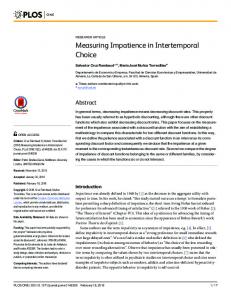
Γ(Δˆ t ) , using these parameters. ˆ ) predicts response time, we estimate To test our hypothesis that Γ(Δ t the linear regression model RTit = b0 + b1t + b2 Γ(Δˆ t ) + ε it .  ˆ ) is highly significant (p < 0.001) and positive in the The effect of Γ(Δ t regression. Figure 1 shows, for each of the three datasets, a plot of RTit − b1t (averaged by trial) against Γ(Δˆ t ) , and the corresponding regression lines. When we average by trial and control for the learning effect,

Γ(Δˆ t ) accounts for 51.2%, 49.8%, and 61.3% of the variance, respectively, in

the Weight, Cognition, and Web studies. When we estimate a different α for each of the different reward categories, the results are even more statistically significant—the corresponding R 2 values are 74.8%, 64.1%, and 70.8%.

4.2. Using response times to predict choice We also estimate the discount function using only the response time data. Specifically, we estimate equation (5) by minimizing the sum of squared residuals (6). Table 2 shows the estimates of αˆ and ωˆ for each of the three datasets, with the choice data columns showing estimates obtained by estimating the choice data model (2) and the RT data columns showing estimates obtained by estimating the RT model (5). Overall, the estimates based on choice data covary closely with the estimates based on response times. The correlation between the αˆ ’s estimated from choice data and the αˆ ’s estimated from response time data is 0.97.7                                                             

5

Response time is a very noisy variable because of the many ways in which it can be affected on any given trial. An example of an outlier is a 59-second response in the Weight study (compared to a mean of 3.4 and SD of 2.8 seconds in this dataset). In other analyses, varying the cutoff point from 2% yielded similar results to those reported here. 6 These estimates are nearly identical to those in Table 1.

  In contrast, the ωˆ  estimates do not move together because of a discrepancy that arises in the

7

ˆ ’s estimated from choice data and the Weight study. The correlation between the ω estimated from response time data is –0.66.  

ωˆ ’s

Additionally, we estimate α and ω for each of the three reward categories. We simply estimate the choice model separately for each reward size category. The response time model is similar to expression (6), except that we allow a distinct discount rate, αˆk , and precision parameter, ωˆ k , for each of the three reward size categories—small, medium, large. Therefore, we seek the vector (bˆ0 , bˆ1 , bˆ2 , αˆ s , αˆ m , αˆl , ωˆ s , ωˆ m , ωˆ l ) that minimizes

∑ [ RT

it

− (bˆ0 + bˆ1t + bˆ2 Γ(Δˆ tk ))]2 , 

it

where

Δˆ tk =

2 ωˆ k

1+ e

Yt − Xt 1+αˆ kτ t

,

and k ∈ {s, m, l} indexes the reward size categories. Table 3 shows the estimates of αˆ and ωˆ for each of the three reward categories in each of the three studies. Again, the estimates based on choice data covary closely with the estimates based on response times. The correlation between the αˆ ’s estimated from choice data and the αˆ ’s estimated from response time data is 0.82.8

4.3. Monte-Carlo horse race As a final test, we compare the predictive power of models estimated using choice data and models estimated using RT data. The idea of the procedure is to estimate α and ω on a subsample of the data using the choice model and also using the RT model, and then compare the out-of-sample predictions for choice data of the two estimated models. This places the RT model at a disadvantage because we are using RT data to make predictions about subsequent choice behavior. We run Monte Carlo simulations with 1000 trials for each of the three studies. On each trial, we choose M subjects randomly and without replacement from the N subjects in the study. Using data from those M subjects we find αˆ choice and ωˆ choice by maximizing expression (2) and we find αˆ RT and ωˆ RT by minimizing expression (6). For the other N–M subjects, we first calculate the mean squared residual from the choice-estimated and RT-estimated parameters. We define the squared residual on trial t of subject i induced by parameters α and ω as                                                              8   The correlation between the ωˆ ’s estimated from choice data and the ωˆ ’s estimated from response time data is 0.94.

 

2

⎡ ⎛ Y ⎞⎤ − X ⎟⎥ , ηˆ = ⎢ dit − FLogit ⎜ ⎝ 1 + ατ ⎠⎦ ⎣ where the variance of the logistic distribution is 1/ ω and where dit is a binary 0-1 variable that equals 1 if and only if subject i chooses the delayed reward on trial t . Next, we calculate the fraction of responses predicted correctly by the two sets of parameters. We say that a response dit is predicted correctly by the 2 it

discounting parameters α and ω if the probability of that response is at least ½ under the choice model:

⎛ Yt ⎞ − X t ⎟ ≤ 1/ 2 .  dit − FLogit ⎜ ⎝ 1 + ατ t ⎠   For each study, we run the Monte Carlo procedure for M = 25, M = 50, and M = 75 and we compute the average of the mean squared residual and the fraction of responses predicted correctly across the 1000 trials. Table 4 shows the mean squared residual and the fraction of responses predicted correctly for the two sets of parameters estimated from choice and RT data, respectively. The discounting parameters estimated using RT data predict out of sample responses almost as well as the parameters estimated using choice data. When we estimate the discounting parameters for each of the three reward categories, the results are qualitatively similar. The difference is that the discounting parameters estimated using RT data do not predict out of sample responses very well when the sample size is small (M = 25). This could be due to the addition of more parameters to the model and the inherently noisy nature of response time data. 5. Conclusion We have used two different approaches to measure preferences. First we adopted the classical approach of inferring preferences from choices. Second we adopted the novel approach of inferring preferences using only response time data. Remarkably, these two approaches yielded nearly identical preference estimates for our aggregated subjects. We conclude that response time data sheds light on both our preferences and on the cognitive processes that execute those preferences. Future work should extend this analysis by asking related questions at the individual subject level. Can response time data also predict variation in preferences at the subject level? Are there sources of data, whether response times or other indices of information processing such as neural activity, that can be used to improve our ability to predict an individual’s choice behavior? Fully exploiting all of the behavioral and physiological information that we can measure during intertemporal choice should enable us to construct more accurate models that yield more novel and precise predictions.

References Ainslie, George (1992). Picoeconomics. New York: Cambridge University Press. Chabris, Christopher F., David Laibson, Carrie L. Morris, Jonathon P. Schuldt, and Dmitry Taubinsky (2008). “Individual Laboratory-Measured Discount Rates Predict Field Behavior.” Forthcoming, Journal of Risk and Uncertainty. Cohen, Jonathan D., Brian MacWhinney, Matthew Flatt, and Jefferson Provost (1993). “PsyScope: A new graphic interactive environment for designing psychology experiments.” Behavioral Research Methods, Instruments, and Computers, 25, 257–271. de Quervain, Dominique J.-F., Urs Fishbacher, Valerie Teyer, Melanie Schellhammer, Ulrich Schnyder, Alfred Buck, and Ernst Fehr (2004). “The Neural Basis of Altruistic Punishment.” Science, 305, 1254–1258. de Wit, Harriet, Janine D. Flory, Ashley Acheson, Michael McCloskey, and Stephen B. Manuck (2007). “IQ and Nonplanning Impulsivity are Independently Associated with Delay Discounting in Middle-aged Adults.” Personality and Individual Differences, 42, 111–121. Edgeworth, Francis (1881). Mathematical Psychics: An Essay on the Application of Mathematics to the Moral Sciences. New York: Augustus M. Kelly. Gabaix, Xavier and David Laibson (2005). “Bounded Rationality and Directed Cognition.” Unpublished paper, Harvard University. Gabaix, Xavier, David Laibson, Guillermo Moloche, and Stephen Weinberg (2006). “Costly Information Acquisition: Experimental Analysis of a Boundedly Rational Model,” American Economic Review, 96, 1043–1068. Henmon, Vivian A.C. (1906) “The Time of Perception as a Measure of Differences in Sensations.” Archives of Philosophy, Psychology, and Scientific Methods, 8. Jaroni, Jodie L., Suzanne M. Wright, Caryn Lerman, and Leonard H. Epstein (2004). “Relationship between education and delay discounting in smokers.” Addictive Behaviors, 29, 1171–1175. Johnson, D.M. (1930). “Confidence and speed in the two-category judgment.” Archives of Psychology, 241, 1–52. Kirby, Kris N., and Nino N. Marakovic (1996). “Delay-discounting probabilistic rewards: Rates decrease as amounts increase.” Psychonomic Bulletin and Review, 3, 100–104. Kirby, Kris N., Nancy M. Petry, and Warren K. Bickel (1999). “Heroin addicts have higher discount rates for delayed rewards than non-drug-using controls.” Journal of Experimental Psychology: General, 128, 78–87.

Loewenstein, George, and Drazen Prelec (1992). “Anomalies in Intertemporal Choice: Evidence and an Interpretation.” The Quarterly Journal of Economics, 107, 573–597. Mazur, James E. (1987). “An adjusting procedure for studying delayed reinforcement.” In M.L. Commons, J.E. Mazur, J.A. Nevin, & H. Rachlin (Eds.), Quantitative Analysis of Behavior: The Effects of Delay and Intervening Events on Reinforcement Value, Vol. 5 (pp. 55–73). Hillsdale, NJ: Erlbaum. Moyer, Robert S., and Thomas K. Landauer (1967). “Time Required for Judgements of Numerical Inequality.” Nature, 215, 1519–1520. Myerson, Joel, and Leonard Green (1995). “Discounting of Delayed Rewards: Models of Individual Choice.” Journal of the Experimental Analysis of Behavior, 64, 263–276. Pinel, Philippe, Stanislas Dehaene, Denis Riviere, and Denis Le Bihan (2001). “Modulation of Parietal Activation by Semantic Distance in a Number Comparison Task.” Neuroimage, 14, 1013–1026. Pinel, Philippe, Manuela Piazza, Denis Le Bihan, and Stanislas Dehaene (2004). “Distributed and Overlapping Cerebral Representations of Number, Size, and Luminance During Comparative Judgments.” Neuron, 41, 983– 993. Rachlin, Howard, Andres Raineri, and David Cross (1991). “Subjective Probability and Delay.” Journal of the Experimental Analysis of Behavior, 55, 233–244. Rubinstein, Ariel (2007). “Instinctive and Cognitive Reasoning: A Study of Response Times.” The Economic Journal, 119, 1243–1259. Samuelson, Paul. (1938). “A Note on the Pure Theory of Consumers’ Behaviour.” Economica, 5, 61–71. Strotz, Robert H. (1957). “The Empirical Implications of a Utility Tree.” Econometrica, 25, 269–280.

Table 1: Discount rates estimated using choice data Weight Cognition Web 0.0090 0.0060 0.0050 Alpha [0.0005] [0.0003] [0.0001] 0.0248 0.0143 0.0104 Alpha small [0.0021] [0.0011] [0.0005] 0.0129 0.0063 0.0056 Alpha medium [0.0010] [0.0005] [0.0002] 0.0065 0.0045 0.0037 Alpha large [0.0006] [0.0003] [0.0001] Notes: Standard errors in brackets. Table 2: Estimated discounting parameters Weight Cognition Web Choice RT Choice RT Choice RT Alpha 0.0094 0.0112 0.0060 0.0043 0.0050 0.0051 [0.0005] [0.0013] [0.0003] [0.0003] [0.0001] [0.0003] Omega 0.0837 0.1545 0.1111 0.0845 0.1199 0.12457 [0.0028] [0.0339] [0.0039] [0.0158] [0.0024] [0.0121] Notes: Standard errors in brackets. For the RT model, observations are clustered by subject and robust standard errors are reported. Table 3: Estimated discounting parameters for each reward category Weight Cognition Web Choice RT Choice RT Choice RT 0.0207 0.0116 0.0147 0.0089 0.0106 0.0065 Alpha small [0.0018] [0.0017] [0.0012] [0.0012] [0.0005] [0.0006] 0.0102 0.0106 0.0061 0.0042 0.0057 0.0066 Alpha medium [0.0009] [0.0020] [0.0005] [0.0006] [0.0002] [0.0006] 0.0061 0.0073 0.0043 0.0040 0.0035 0.0055 Alpha large [0.0006] [0.0013] [0.0004] [0.0005] [0.0002] [0.0005] 0.1509 0.0945 0.1917 0.1345 0.1898 0.1144 Omega small [0.0079] [0.0368] [0.0106] [0.0262] [0.0059] [0.0176] 0.0804 0.0435 0.1125 0.0773 0.1195 0.0547 Omega medium [0.0046] [0.0156] [0.0066] [0.0152] [0.0040] [0.0082] 0.0699 0.0395 0.0892 0.0682 0.0979 0.0471 Omega large [0.0038] [0.0154] [0.0053] [0.0140] [0.0034] [0.0076] Notes: Standard errors in brackets. For the RT model, observations are clustered by subject and robust standard errors are reported.

Table 4: Monte-Carlo results Estimation Study Sample Size

Mean SR (Choice) 0.1344 Weight [0.0002] 0.1163 75 Cognition [0.0002] 0.1152 Web [0.0000] 0.1349 Weight [0.0001] 0.1168 50 Cognition [0.0001] 0.1155 Web [0.0001] 0.1361 Weight [0.0001] 0.1178 25 Cognition [0.0001] 0.1165 Web [0.0001] Notes: Standard errors in brackets.

Mean SR (RT) 0.1347 [0.0003] 0.1242 [0.0002] 0.1161 [0.0001] 0.1378 [0.0006] 0.1252 [0.0002] 0.1169 [0.0001] 0.1490 [0.0018] 0.1292 [0.0005] 0.1204 [0.0003]

Correct (Choice) 0.8338 [0.0004] 0.8471 [0.0005] 0.8390 [0.0002] 0.8329 [0.0003] 0.8475 [0.0005] 0.8404 [0.0002] 0.8282 [0.0004] 0.8477 [0.0005] 0.8418 [0.0003]

Correct (RT) 0.8315 [0.0005] 0.8352 [0.0003] 0.8400 [0.0002] 0.8263 [0.0007] 0.8362 [0.0003] 0.8414 [0.0003] 0.8181 [0.0010] 0.8385 [0.0004] 0.8427 [0.0003]

  Figure 1: Plots of RT − b1t versus Γ for each of the three studies