Measuring microscopic viscosity with optical tweezers as a confocal probe Boaz A. Nemet and Mark Cronin-Golomb
We demonstrate, what is to the best of our knowledge, a new method for studying the motion of a particle trapped by optical tweezers; in this method the trapping beam itself is used as a confocal probe. By studying the response of the particle to periodic motion of the tweezers, we obtain information about the medium viscosity, particle properties, and trap stiffness. We develop the mathematical model, demonstrate experimentally its validity for our system, and discuss advantages of using this method as a new form of scanning photonic force microscopy for applications in which a high spatial and temporal resolution of the medium viscosity is desired. © 2003 Optical Society of America OCIS codes: 180.5810, 180.1790, 170.3880, 140.7010.
1. Introduction
In the study of colloidal suspensions and polymer physics and in molecular and cell biology it is often desirable to have a direct observation in real time of the changes in the local viscosity that affect the dynamics of such objects as colloidal particles, cellular organelles, and macromolecules. For example, in cell biology the study of intercellular signaling is advancing rapidly.1 Tissue function heavily depends on the ability of neighboring cells to communicate. Cells communicate primarily by secreting cytokines, which are soluble proteins that diffuse through the surrounding medium and ultimately bind to receptors where the signal is received.2 These signals modulate the functional activities of individual cells and tissue. The diffusion of the signaling molecules is governed by the gradients in concentration and viscosity in the intercellular medium. Mapping the viscosity in such a medium is therefore important for understanding the processes involved in intercellular signaling that could have considerable implications for the interpretation of organ physiology and for tissue engineering. When this research was performed the authors were with the Department of Biomedical Engineering, Tufts University, 4 Colby Street, Medford, Massachusetts 02155. M. Cronin-Golomb 共
[email protected]兲 is currently with Biological Sciences, Columbia University, 1002 Fairchild Center, MC 2435, New York, New York 10027. Received 11 June 2002; revised manuscript received 2 December 2002. 0003-6935兾03兾101820-13$15.00兾0 © 2003 Optical Society of America 1820
APPLIED OPTICS 兾 Vol. 42, No. 10 兾 1 April 2003
Recently we have demonstrated3 that quantitative mapping of viscosity distributions can be achieved with a high spatial and temporal resolution by using a method that probes such viscous environments by use of photonic force. In that previous research, we have obtained a detailed map 共0.5-m resolution兲 of the relative viscosity in the extracellular environment of a high-molecular-weight-biopolymer-producing cell of Aureobasidium pullulans. In this paper we expand on the experimental and theoretical basis of this method and discuss advantages, limitations, and extensions, such as dynamic light scattering and flow and force measurements. Optical tweezers have proved a powerful tool in the investigation of biological systems, and many intriguing experiments have been performed on the physics of single molecules 共for reviews see, for example, Ref. 4 and references therein兲. Optical tweezers allow noninvasive probing and manipulation of cellular environments. In our device, we use the trapped particle as the probe to measure the local viscosity. We approach the detection of that particle in what is to the best of our knowledge, a new way that employs confocal optics. The use of confocal geometry is a natural choice since the setup for optical tweezers is so similar to the setup for confocal microscopy. It results in sensitive detection and facilitates fast scanning and beam steering. In this design, the optical tweezers is also the probe beam of an inverted confocal microscope. The trapped object scatters light from the focal region and is confocally detected through a pinhole 共or an optical fiber兲 placed in an image plane. To measure viscosity, we force the trapped particle periodically by moving the laser
tweezers back and forth across it at frequencies in the kilohertz range at small amplitudes 共⬃100 nm兲. This forcing results in periodic motion of the particle with the same frequency as the driving frequency and a phase lag due to the drag. By measuring this phase lag, we can determine the characteristic time constant of the motion, which is proportional to the medium viscosity. If at the same time the particle is moved through the field of view, a spatial map of the viscosity is obtained. If this is repeated at different times and at different depths, we have a full threedimensional 共3-D兲 mapping of the viscosity distribution and evolution. The outline of the paper is as follows. In Section 2 we describe the experimental procedure and the optical setup. In Section 3 we elaborate on some of the optical design considerations. In Section 4 we develop the physical model from first principles to the analytical solution, which is the main result and the basis of the measurement technique. The analytical solution is derived from a linearized equation under nonrestrictive simplifying assumptions. In Section 5 we show results from theoretical research on the signal-to-noise ratio 共SNR兲 and its dependence on the various parameters, as well as a comparison with experimental SNR. In Section 6 we show the change in trap stiffness with depth within the specimen and give an interpretation of it in terms of optical aberrations. Section 7 is the discussion. In Subsection 7A we review some of the existing methods and show similarities to and differences from our own method, and in Subsection 7B we discuss extensions to the method, such as localized dynamic lightscattering microscopy and flow measurement. Finally, we conclude in Section 8 with a summary of the main results, followed by an appendix detailing the signal-to-noise calculations. 2. Experimental Setup and Procedure
Figure 1 shows a schematic diagram of the optical layout. Linearly polarized light from a continuous wave 共cw兲 Ti-Sapphire laser 共Spectra Physics 3900, Mountain View, California兲 is focused by an objective lens 共Edmunds Micro Plan 100⫻ 1.25 NA, Edmund Industrial Optics, Barrington, New Jersey兲 to form the optical trap in the sample. An acousto-optic deflector 共AOD兲 共Isomet 1205C-2, Isomet Corporation, Springfield, Virginia兲 sets the beam into periodic motion, causing a trapped probe bead to oscillate in the transverse direction 共only the first-order diffracted beam is used, whereas the zero order is blocked兲. Backscattered light from the trapped particle is descanned by the AOD and is detected confocally by placement of a pinhole or single-mode fiber near an image plane in front of the photodetector.5 The trapped particle appears as an object in the focal point of the laser beam. As the particle moves about in the trap, the confocal signal varies. For a wellaligned TEM00 Gaussian beam the signal is maximum at the center and decreases as the particle moves away from the focal region. Because of the hydrodynamic drag, the particle lags behind the os-
Fig. 1. Experimental layout. The pinhole 共P兲 is placed in an image plane of the object, forming the confocal detection. These conjugate planes are marked with #. The AOD is placed at an optically conjugate plane of the back aperture of the objective lens 共OL兲. The conjugate planes are marked with *. Two galvanometer SMs are placed in another such conjugate plane 共*兲. The LIA drives the AOD with a sinusoidal waveform and measures the magnitude and phase of the APD signal at the second-harmonic frequency. The scene is viewed with a CCD camera in transmission through the dichroic mirror 共DM兲 that has high reflectivity in the IR. SL1 is the scan lens.
cillating beam. As a result, the beam traverses the particle twice in each cycle, and the confocal signal peaks twice per cycle, yielding a signal at the second harmonic. A digital lock-in amplifier 共LIA兲 measures the phase difference between the confocal signal and the second harmonic of the spatial oscillation frequency of the trap. The phase is then used to determine the local viscosity with the model in Section 4. The frequency and amplitude of the oscillations are set digitally by the LIA, which is used also as the function generator to supply the sinusoidal voltage to modulate the AOD carrier frequency.6 Two orthogonal scanning mirrors at location SM in Fig. 1 have four functions: 1. They can be used to form an image by x–y raster scan in the conventional use of the scanning confocal microscope. 2. They can be used to drag the particle in the sample, and with our measurement technique, to obtain an image of the viscosity. 3. They can be used to control and manipulate the laser trap’s position. To accomplish this, we use our own computer software that integrates the CCD camera, the frame grabber, and the galvanometer drivers and allows us to take measurements of the viscosity at desired locations in the field of view. We use the computer mouse for the manipulation of the trap in real time by moving a cross hair on the computer screen. The mouse coordinates are translated into mirror coordinates by a linear transformation and sent through the serial port to the x–y galvanometer drivers. 4. They can be used to manipulate biological cells, possibly for sorting, in applications in which the viscosity measurement is used as an indicator of highproducing cells. 1 April 2003 兾 Vol. 42, No. 10 兾 APPLIED OPTICS
1821
3. Optical Design
Optical tweezers and confocal geometry combine in a very natural and almost obvious way that is easy to implement. This arrangement is appealing for two main reasons: 共i兲 for detection purposes in that the particle whose position we wish to detect is automatically aligned with the beam since we use the same laser beam for both detection and trapping and 共ii兲 for steering capabilities in that the same optical design considerations that need to be addressed during construction of a steerable laser trap appear during construction of a confocal scanning laser microscope. The confocal design problem is how to move the beam at the sample plane without it walking off the back aperture of the objective lens, which would cause a reduction in light intensity and severe aberrations. By solving the confocal design problem, we also solve the problem for the steerable tweezers. The standard solution in designing a confocal microscope is to place the scan mirror or any other steering device 共e.g., AOD兲 at an optically conjugate plane to the back focal plane of the objective lens.7,8 In our case, a slight modification is to image the steering device onto the back aperture of the objective lens.9 This facilitates laser scanning with minimal loss of light and minimum aberrations since minimal lateral translation of the beam occurs at such a plane 关marked with an asterisk 共*兲 in Fig. 1兴. In practice this is implemented with a scan lens 共SL兲 that has three functions: 共i兲 imaging the SM onto the objective lens back aperture; 共ii兲 focusing the laser beam to a spot at a primary image plane, which is translated to a spot at the object plane by the objective lens 共the optical trap兲; and 共iii兲 overfilling the objective lens aperture by approximately 30% to ensure a diffraction-limited spot size,7 as required for a 3-D stable single-beam trap. Therefore, the focal length of the SL must satisfy the condition to yield the desired magnification for the beam width at the objective lens aperture. The three conditions can be stated in mathematical form as a system of three simultaneous equations for the parameters f1, u1, and v1, which are respectively the SL focal length, the SM to SL1 distance, and the SL to objective aperture distance. 共i兲 共ii兲
l兾f 1 ⫽ l兾u 1 ⫹ l兾v 1, v 1 ⫽ 150 mm ⫹ f 1,
共iii兲 v 1兾u 1 ⫽ M, where we used for 共i兲 the image formation formula for a thin lens; for 共ii兲, according to the DIN standard, the distance from the back aperture of the objective lens to the primary image plane is 150 mm, and we assumed that the beam is collimated before the SL; for 共iii兲 the magnification M is known from the width of the beam before the lens and the size of the objective lens pupil. For example, with a 2-mm-diameter beam and 6-mm-diameter pupil, we get M ⫽ 1.3 ⫻ 6兾2 ⫽ 3.9. 1822
APPLIED OPTICS 兾 Vol. 42, No. 10 兾 1 April 2003
Note that if the beam is not collimated before the SL then the calculation is a little more complicated, but we can still solve a system of simultaneous equations, taking into consideration the beam divergence, to obtain the information on the position of the SL and its focal length. Another consideration is the diameter of the SL. Since this lens also collects the backscattered light from the trapped object 共or alternatively the fluorescence light兲, it should be as large as possible for high throughput to optimize the amplitude of the detected signal. 4. The Model
In confocal detection we receive a signal from the particle whenever it is in the focal region of the trapping beam. We therefore develop a mathematical model for u ⫽ x ⫺ p, where x is the transverse position of the particle and p is the trap position.10 We expect a peak in the signal whenever u ⫽ 0. In the following, we describe the main features of our physical model that relate the measured phase and the microscopic viscosity. A particle trapped by the light force finds itself in, to a good approximation, a quadratic potential well 共in the transverse direction兲. In this paper, we will consider the analysis of Newtonian fluids, noting that it is straightforward to make an extension to cases for which the Stokes– Einstein relation may be generalized to account for viscoelasticity.11 In that case, the measured magnitude of the viscosity becomes frequency dependent. The generalized analysis is described elsewhere. The one-dimensional 共1-D兲 equation of motion of a particle in a viscous Newtonian fluid undergoing Brownian motion in an oscillating harmonic potential is ␥
dx ⫹ 关 x ⫺ p共t兲兴 ⫽ L共t兲, dt
(1)
where x is the particle’s position, p共t兲 is the timedependent position of the trap p共t兲 ⫽ a sin共0 t兲, and ␥ is the hydrodynamic drag coefficient. For a sphere far from any surface, ␥ is given by the Stokes formula 6r, where r is the radius of the sphere and is the dynamic viscosity.12 L共t兲 is the Langevin forcing function associated with Brownian motion, and is the tweezers spring constant. The inertial term 共mass times acceleration兲 that would normally be included on the left-hand side of Eq. 共1兲 can be neglected on the grounds that in common fluids the motion of micrometer-sized particles takes place at a small Reynolds number where viscous drag dominates inertial forces.12 In terms of u, Eq. 共1兲 becomes ␥
du ⫹ u ⫽ ⫺␥a 0 cos 0 t ⫹ L共t兲. dt
(2)
The assumption that the particle stays near the center of the trap also allows us to express the confocal signal as proportional to 1 ⫺ ␣u2, where ␣ is an expansion coefficient. In our measurement tech-
Fig. 2. Experimentally measured second-harmonic phase for 1.9-m diameter silica microsphere in water, for varying laser power 共15 to 60 mW at the sample兲 at a constant frequency of 600 Hz 共䊐兲 and for varying frequency 共200 to 2000 Hz兲 at a constant power of 46 mW 共E兲. Each measurement of 2 is the average of 512 samples from the LIA 共sampled at 64 Hz兲. The LIA time constant was 100 ms, corresponding to NEBW of 0.78 Hz. The errors in 2 from the standard deviations are smaller or equal to the size of the symbols and are omitted for clarity. Both sets of measurements are plotted together after a linear regression fit was done on each set separately to obtain b. The abscissa parameter 0 is calculated from 0 b兾P. The solid curve shows the theoretical curve for which the x axis is cot共2兾2兲. Inset: Linear regression fit to the frequency data, ⫽ slope ⫽ 1.290 ⫾ 0.003 ms with a correlation coefficient 0.99974. From a similar linear regression 共not shown兲, we obtain for the power measurements b ⫽ 59.48 ⫾ 0.27 J with a correlation coefficient 0.999.
nique, the dominant forcing comes from the periodic motion of the tweezers, and we detect only the motion associated with this periodicity in a narrow band set by the time constant of the LIA. The contribution of the Brownian motion in such a narrow band of frequencies is small but is the main source of noise. Therefore we solve the equation without the Langevin term and consider it only later in the discussion of the SNR. The solution of Eq. 共2兲 is u共t兲 ⫽ ⫺u 0 sin共 0 t ⫹ 1兲,
(3)
where 1 ⫽ cot⫺1 0 共 ⫽ ␥兾 is the relaxation time兲 and u0 ⫽ a0兾关1 ⫹ 共0兲2兴1兾2. We find that the phase of the second harmonic appearing in u2 is given by 2 ⫽ 2 1 ⫽ 2 cot⫺1 0.
(4)
We verified the validity of our model by measuring the second-harmonic phase 共2兲 as a function of the laser power 共P兲 and the trap oscillation frequency 共0兲. Figure 2 shows the results from two sets of measurements on a 1.9-m-diameter silica microsphere in water. In one set of measurements, we keep the frequency of the oscillations constant 共600 Hz兲 while varying the laser power between 15 and 60 mW. In the second set, the laser power is kept constant 共46 mW at the sample兲 while the oscillation
frequency is varied between 200 and 2000 Hz. If the theory is correct and the trap spring constant is approximately proportional to power ⫽ 0 P, where P is the laser power, then decreasing the power is equivalent to increasing the oscillation frequency. We can therefore collapse the data on one graph and plot both sets as a function of the normalized time constant 0. The parameter b, which is defined by b ⫽ P, has units of energy and is a characteristic constant of the physical conditions of the experiment. It is independent of the frequency of the oscillations and the laser power 共note that by definition is inversely proportional to , which by our assumption is proportional to P兲. This independence means that b remains constant for a given particle 共size, shape, and refractive index兲, the fluid medium 共viscosity and refractive index兲, and the optical microscope system being used 共objective lens, laser mode, wavelength, etc.兲. We interpret it as the amount of electromagnetic energy needed to make an unforced particle relax to 1兾e of any initial displacement from the center of the trap. The greater the optical power in the tweezers beam, the faster a trapped particle relaxes to the potential minimum. For the set of measurements in which the power was varied, we first get b ⫽ 59.48 ⫾ 0.27 J from the best fit to the slope of 0 ⫻ tan共2兾2兲 versus P. For the set of measurements in which the frequency was varied, we get ⫽ 1.290 ⫾ 0.003 ms from the best fit to the slope of cot共2兾2兲 versus 0 共see inset in Fig. 2兲, and using P ⫽ 46 mW we have b ⫽ 59.73 ⫾ 0.15 J.13 For this set of measurements the trap constant is ⫽ 1.38 ⫻ 10⫺5 ⫾ 3.2 ⫻ 10⫺8 N兾m, where we used ␥ ⫽ 1.79 ⫻ 10⫺8 kg兾s from the known viscosity and particle size. The main graph in Fig. 2 shows 2 versus 0 for both data sets for which we used 59.73 J for the value of b. Also plotted is the theoretical line cot共2兾2兲. One of the advantages of our technique is that it allows us to optimize the sensitivity of the measurement by varying P, 0, or both, enabling us to make measurements over a large range of medium viscosities without changing the apparatus while keeping the SNR high, as can be seen from Eq. 共5兲 below. The results show that Eq. 共4兲 holds and reaffirms the proportionality assumption between and laser power P. We also see that the parameter b is the same for both sets of measurements, which shows it is independent of both 0 and P as can be seen from Eq. 共5兲 below. Changes in the value of b thus represent real changes in the medium viscosity and can be used to monitor biological, physical, or chemical processes. To deduce the absolute viscosity of the fluid we need to measure the trap stiffness independently. This could be done either by another method, such as the escape force method,14 or by use of a standard medium for calibration. In many cases, only relative viscosities need to be determined, for example, in a cell-sorting application in which we are interested in the cell producing the highest viscosity in a given population. In cases in which an absolute measure1 April 2003 兾 Vol. 42, No. 10 兾 APPLIED OPTICS
1823
ment is required, we can calibrate the system using materials of known viscosity, such as water or glycerol. Calibration against standards is preferred over ab initio calculations because we do not need to take into account the physical parameters of the probe particle or the inaccuracies of the available theory regarding the trap stiffness . Once calibration is done, we need only one measurement of the phase 2 to determine the viscosity of a given medium. If 3-D measurements are needed in an inhomogeneous medium, then calibration of the trap stiffness needs to account for the variation in depth inside the medium 共see Section 6兲. We note that for accurate mapping of the viscosity, it is important that the variation in refractive index be small, such that the trap stiffness does not vary appreciably. If this is not the case, then the measurement is complicated by the inability of our method to decouple the change in index from the change in viscosity. 5. Signal-to-Noise-Ratio
A full analysis of the SNR of our measurement technique is given in Appendix A. Here we present the main ideas and the basic result from that research, which we believe is pertinent to understanding the advantages of the technique. The approach in the calculation is to look at the equation of motion of the particle and to include the Brownian motion as the main source of noise in the measurement under the assumption that the detector is not limited by the light intensity. The thermal excitation adds a randomly fluctuating component to the position of the particle. Since we are dealing with a linear system, the solution for the relative position u is a superposition of the purely sinusoidal function with low-pass filtered noise 共the Lorentzian spectrum兲. A quadratic approximation to the confocal point-spread function 共PSF兲 is used to relate the particle’s displacement to the signal voltage. Since the detection is nonlinear in relative displacement u, we find a modulation of the thermal noise at frequency 0 by a signal–noise cross term that is the main source of noise at the narrow measurement band 共2⌬兲 centered at 20. These considerations allow us to obtain an analytical expression for the viscosity SNR defined as SNR ⬅ 兾⌬, where ⌬ is the rms fluctuation of the viscosity , SNR ⫽
冉 冊 冉 冊
共 0兲 2 a 共 0兲 2 ⫹ 1 k B T
1兾2
1 8⌬
1兾2
.
(5)
We first note that the SNR is proportional to the ratio between the amplitude of the oscillation a and the rms thermal fluctuations 共kB T兾兲1兾2. We also note that for long time constants or high trap oscillation frequencies, the SNR approaches a constant value. We can rearrange Eq. 共5兲 and write SNR ⫽ 1824
SNR⬁ , 1 ⫹ 共 0兲 ⫺2
APPLIED OPTICS 兾 Vol. 42, No. 10 兾 1 April 2003
Fig. 3. SNR of the viscosity measurement for 0.9-m-diameter silica microsphere in water with 18 mW of laser power at 815 nm and a constant NEBW of 2.6 Hz. The characteristic frequency fc ⫽ 585 Hz is indicated by the dotted line. The solid curve is the theoretical curve 共see text for details兲.
where
冑
1 a F springrms 2 ⬁ ⫽ . SNR ⫽ 关2␥k B T共2⌬兲兴 1兾2 F Langevinrms
(6)
At high viscosities 共0 ⬎⬎ 1兲, for constant laser power, the sensitivity in the measurement of the viscosity saturates at a value 共SNR⬁兲 that is given by the ratio of the rms spring force of the laser trap to the rms Langevin force in the bandwidth 2⌬. In the other extreme in which 0 ⬍⬍ 1, the SNR increases like the square of the viscosity. We see that if we operate in the regime of high viscosity, we can reach high SNR where the only limiting factor is the amount of laser power that we have available 共since is proportional to the laser power兲. However, if speed of measurement is of concern then, as shown in Eq. 共5兲, we are also limited by the bandwidth of the LIA. In a typical experiment the laser power at the sample plane is 18 mW at 815-nm wavelength. We use a 0.9-m-diameter silica microsphere in water 共 ⫽ 1 ⫻ 10⫺3kg兾m兾s兲, an amplitude a ⫽ 100 nm, ⫽ 3.12 ⫻ 10⫺5 N兾m, and a bandwidth of 2.6 Hz, which is the noise-equivalent bandwidth 共NEBW兲 of the LIA when it is set with a time constant of 30 ms and a filter slope of 24 dB兾octave.15 Figure 3 shows the SNR measured under these conditions for a range of oscillation frequencies 共the laser power and measurement bandwidth were kept constant兲. The time constant ⫽ 0.272 ⫾ 0.0014 ms was found from a fit to Eq. 共4兲. Values for the experimental SNR were calculated with SNR ⫽ 共sin 2兲兾⌬2 关derived by the definition of SNR and by Eq. 共4兲兴, in which we used the mean and standard deviation from 1024 samples of 2 共sampled at 64 Hz兲 for each data point.16 The theoretical SNR is also shown by the
solid curve, where we fitted Eq. 共5兲 to the data with the free parameter SNR⬁. The value of SNR⬁ from the best fit to all the data points is 65, whereas the theoretical SNR⬁ calculated with the parameters above is 46.5. The discrepancy might be accounted for by the uncertainty in the value for the oscillation amplitude a and variations in the laser output power. The SNR sets a limit to the dynamic range of viscosities that can be accurately measured for a given optical power. We estimate the dynamic range using Eq. 共5兲 to be of the order of 2 decades. For a fluid of viscosity 200 times that of water, the SNR drops to 兾⌬ ⫽ 5. This estimate assumes the following parameters: a 0.9-m-diameter silica microsphere, an 800-nm trap wavelength, a ⫽ 2 ⫻ 10⫺5 N兾m trap constant, an f ⫽ 1100 Hz tweezers oscillation frequency, a trap oscillation amplitude 0.14 m, and a lock-in time constant 100 times the period of oscillation of the trap 共⌬ ⫽ 5 rad兾s兲. Note that a larger dynamic range can be achieved by one’s increasing the laser power or by one’s reducing the detection bandwidth, but the latter comes at the expense of reduced speed. From Eq. 共5兲 we see that by increasing the oscillation amplitude we can increase the SNR and as a result the dynamic range. Finally, we note that the SNR in the viscosity measurement is equivalent to the SNR in since
SNR ⫽
␥ ⫽ ⫽ . ⌬ ⌬␥ ⌬
If we know ␥ from a priori knowledge of particle radius and medium viscosity, then this equivalence of SNRs means that we can have a high-precision calibration of the transverse trap stiffness. For example, for an SNR of 65 in water, we get the value of with a precision of 1兾65 or 1.5% by a single measurement of the second-harmonic phase, which takes about a second to complete.
6. Trap Stiffness
In confocal microscopy 3-D visualization is made possible by the depth discrimination property.7,17 This property allows us, in this setup, to drag the probe particle to deeper depths far from the cover glass and to obtain 3-D information of the viscosity distribution in a given medium. To do that, however, we need to first determine how the transverse trap stiffness 共兲 varies along the axial 共z兲 dimension. A complication that arises is the fact that objects moving close to a surface experience an increase in the drag due to the no-slip boundary condition. For a sphere moving in a viscous fluid near a surface, it was shown in Ref. 18 that the modification to the Stokes drag coefficient is given by a multiplicative factor involving the ratio of
Fig. 4. Trap stiffness as a function of distance from the cover glass. is calculated by means of ␥⬁兾共䊐兲 and by means of ␥⬁g共z兲兾 共E兲 with Brenner’s formula for the correction near the two surfaces 共see text兲. We obtain from measurements of the second-harmonic phase for the following conditions: 1.9-mdiameter silica microsphere in water ␥⬁ ⫽ 6r ⫽ 1.79 ⫻ 10⫺8 kg兾s, constant laser power of 29 mW at the sample, 815-nm wavelength, constant frequency of oscillations of 500 Hz, objective lens 100⫻ magnification, and 1.25 NA oil immersion. Solid lines are drawn to guide the eye. Each data point is the mean of 512 samples 共sampled at 64 Hz where the time constant of the LIA was 300 ms and 0.26 Hz NEBW兲. Error bars obtained from the standard deviations.
the radius of the sphere 共r兲 and its distance from the surface 共z兲,
冋
g共 z兲 ⫽ 1 ⫺ ⫺
冉冊 冉冊 冉 冊册 9 r 1 r ⫹ 16 z 8 z
1 r 16 z
5 ⫺1
3
⫺
冉冊
45 r 256 z
.
4
(7)
Figure 4 shows results from a set of measurements of the second-harmonic phase taken at different distances 共z兲 from the bottom cover glass. We increased z in steps by moving the objective lens assembly using a stepper motor actuator. We plot as a function of z by calculating ␥⬁兾, where ␥⬁ ⫽ 6r ⫽ 1.79 ⫻ 10⫺8kg兾s is the value for the Stokes drag for 1.9-m-diameter silica microsphere in water far from any surface. We also plot after correcting for the drag near the bottom 共coverslip兲 and top 共glass slide兲 surfaces by calculating ␥⬁g共z兲兾. The correction factor is only important close to the surface, where the distance is of the order of the particle’s radius.19 The figure reveals a complicated relation of the transverse trap stiffness dependency on z. We find that the trap stiffness initially increases approximately linearly with distance from the coverslip. It then falls sharply in the middle of the chamber and then stays relatively constant until another final decrease close to the top surface. The variation in trap stiffness, we believe, originates in the severe spherical aberrations that result from the use of an oil1 April 2003 兾 Vol. 42, No. 10 兾 APPLIED OPTICS
1825
immersion objective lens. When the focus is immediately below the coverslip, there are minimal aberrations, but as the focus is moved further deep into the water, the ray paths do not converge since off-axis rays experience more refraction at the coverslip–medium interface.8 This results primarily in a decrease in axial trap efficiency, which moves the equilibrium position of the particle in the z direction further down the beam. This decrease, in turn, results in a change in transverse trapping since the particle experiences a different lateral gradient in the new z position.20,21 The interpretation of the trap stiffness measurements is not straightforward and is sometimes even counterintuitive.4 We find it rather surprising that the observed transverse trap stiffness actually increases with depth. This result suggests that as we increase z, the particle experiences a sharper gradient in intensity in the lateral 共x–y兲 plane. Whatever the reason for this dependency, it is clear that it must be considered when the method is applied to measure viscosity in an inhomogeneous medium at different depths. 7. Discussion A.
Comparison with Other Methods
To the best of our knowledge, there has been no previous study of optical tweezers as a confocal probe to monitor the position of a particle relative to the center of an oscillating trap or the associated use of second-harmonic phase detection to obtain . Visscher and Brakenhoff22 combined optical tweezers with a confocal microscope but not in the same way and not for the same purpose. In that arrangement there were two separate paths for confocal imaging and laser trapping with two different objective lenses from opposite sides of the sample. Their device attempted to use the laser to keep an object trapped and to manipulate it while at same time supplying confocal scanning imaging of the field of view to a CCD camera. A special trap objective lens was constructed to allow the 3-D manipulation of the object by moving the effective lens inside the objective lens itself. Their device does not make use of confocal detection to measure the displacement of the particle from the trap center. The confocal part is used strictly for 3-D sectioning, and there is no attempt to measure . There are numerous reviews in the literature of photonic force calibration techniques.4,14,23 Florin et al.23 divide these methods into two main categories: one, calibration against known forces 共such as Stokes friction and gravity兲 and two, analysis of thermal fluctuations. We can look at another subdivision for methods that require a well-calibrated position sensor of the trapped particle and methods that instead measure temporal changes in the signal and do not require an absolute distance measurement. Visscher et al.14 describe and compare the following methods: escape force, drag force, step response, power spectrum, and equipartition. With the exception of the last, all methods essentially measure . The 1826
APPLIED OPTICS 兾 Vol. 42, No. 10 兾 1 April 2003
trap stiffness is derived from knowledge of ␥ 共 ⫽ ␥兾兲, and one obtains force measurements by assuming a Hookian spring force for the trap and using a position sensitive detector. For accurate force measurements, both the trap stiffness and the position signal need to be well calibrated. For position detection most methods use a quadrant 共or split兲 photodiode placed in an image plane. In one example, Florin et al.23 use such detection to measure the position and use Boltzmann statistics to analyze the thermal noise and obtain the shape of the potential well of the trap. They deduce from the best fit to harmonic potential. To make a fair comparison requires accounting for the purposes of each technique so that its advantages and disadvantages can be evaluated. Although our method could be used to calibrate the trap stiffness, it was developed specifically to be fast and robust for scanning the laser beam 共as in confocal microscopy兲 and not for absolute position detection with the nanometer resolution, needed, for example, for picotensiometry. Advantages of our technique stem from the following: • The simplicity of the optical setup—its automatic alignment property and the solutions it provides for laser beam manipulation. • The active use of photonic force to move the particle at high frequencies 共kilohertz range兲 by the AOD. • The highly sensitive detection of the particle’s displacement from the trap center. • The scanning capability and the large photon fluence at the detector, all resulting from the confocal geometry. • The use of a digital LIA to accurately measure the second-harmonic phase with a narrow noise bandwidth, yielding a high SNR while maintaining a short data-acquisition time. • The fact that, unlike the techniques of power spectrum and Boltzmann statistics, there is no need to fit the data in our measurement. This factor allows for a real-time measurement without complicated analysis.
Methods belonging to the category of thermal fluctuations, use the wide Brownian spectrum of the trapped particle to deduce the stiffness from the Lorentzian spectrum corner frequency fc. The random fluctuations in the position of the particle are monitored typically by a position-sensitive quadrant photodiode arrangement.14,24,25 These methods could be used to measure microscopic viscosity in a similar way to that of our device. However, they are not suitable for fast scanning for two main reasons. First, they are not suited for beam scanning since as the trapping beam moves, the image of the particle moves off the center of the split photodiode. Therefore, they can scan the sample only using motors or piezoelements on the microscope stage, which are much slower than moving the laser itself. Secondly,
these methods are not fast owing to the long integration period inherent in a wideband spectral measurement. In most methods employing the positionsensitive detector, the trapped particle acts like a microlens that collimates the light. Different size particles have different effects on the light path, and as a result, realigning and recalibrating the position sensor is needed every time a new type of particle is trapped. In our opinion the use of an active periodic forcing, rather than the use of the Brownian spectrum, is more adaptive to environmental constraints; large variations in the medium viscosity can be handled by the ability to change the trap stiffness or oscillation frequency. Our method does not rely on thermal excitations to supply the forcing; it shifts the measurement away from the thermal Lorentzian noise and the low-frequency mechanical noise spectra to a much higher frequency of our choice. For example, without special isolation from mechanical noise and sound, vibrations from environmental disturbances would be picked up by the system and would appear in the power spectra as peaks at the harmonic frequencies. The technique described by Valentine et al.26 is the one that is most similar to ours. They also use an active force rather than a thermal noise and measure the response of a particle to periodic forcing by optical tweezers employing lock-in detection. The main difference between their device and ours is the use of a split photodiode and not confocal detection for the particle’s position. In addition, it is slower, as can be seen by considering the SNR. Using similar considerations to the ones leading to Eq. 共5兲, we calculated the SNR for the case of Valentine’s device 共see Appendix A兲 where we define c ⫽ 1兾: SNRValentine ⫽
冉 冊 冉 冊
0 c a 2 2 0 ⫹ c kB T
1兾2
c 8⌬
1兾2
.
(8)
The ratio between the SNRs of the two methods is simply 0. SNRConfocal ⫽ 0. SNRValentine
(9)
The advantage of applying high-oscillation frequency to the trap is the ability to make a quick measurement while integrating over many periods. This ability leads to the possibility of fast scanning viscosity microscopy.3 The shorter the integration time, the larger the measurement bandwidth. If we adjust the measurement bandwidth 共⌬兲 to be proportional to the tweezers oscillation frequency 共0兲, the SNR is maximized when 0 ⫽ 公3 for the confocal case and when 0 ⫽ 公1兾3 for Valentine’s method. In Fig. 5 we compare the signal-to-noise behavior of Valentine’s device to ours by plotting the SNRs as a function of frequency using Eqs. 共5兲 and 共8兲. Notice that at low frequencies, Valentine’s method is supe-
Fig. 5. Comparison of the theoretical SNR of the viscosity measurement for the confocal detection 共our device兲 and for the splitphotodiode position detection 共Valentine’s device兲. The measurement bandwidth was taken to be proportional to the oscillation frequency. The SNR of the two methods are equal at the characteristic frequency, which was taken to be fc ⫽ 585 Hz 共as used in Section 5兲. The confocal SNR peaks at 公3 fc ⫽ 1013 Hz, whereas Valentine’s SNR peaks at 1兾公3 fc ⫽ 338 Hz. The three frequencies are marked with dotted lines. From left to right these are the frequency of peak SNR for Valentine’s device, the frequency where the SNR of Valentine’s device is equivalent to ours, and the frequency of peak SNR for our device.
rior to ours, since the split photodiode ac signal is large when the bead can follow the trap, but the confocal ac signal is small since the particle stays close to the center of the trap. But at high frequencies, required for high data-acquisition rates, the confocal detection SNR significantly exceeds that of the split photodiode method. The SNR decreases as 0⫺1兾2 in the confocal case but as 0⫺3兾2 in the split photodiode case. Florin et al.27 combine optical tweezers and a twophoton fluorescence microscope to measure surface topography and stiffness. While they do not actively move the particle, they detect its position in a way similar to a confocal microscope. Their method eliminates the need for the pinhole, but it is limited by the need for an ultrafast laser. Meller et al.28 proposed the approach of localized dynamic light scattering 共LDLS兲 on a particle trapped by optical tweezers. They compute the temporal autocorrelation function 共ACF兲 of the scattered intensity and relate it to the particle position correlation function to obtain . In comparison with the other methods discussed, their method does not use a position sensor, but it requires careful alignment of the probe fiber and isolation from low-frequency noise that otherwise decreases the SNR. In addition, it requires a long integration time for the statistics to be reliable 共a few minutes as compared with less than a second for our method3兲. There are, however, advantages in getting the position ACF, which can reveal the existence of more than one relaxation time, 1 April 2003 兾 Vol. 42, No. 10 兾 APPLIED OPTICS
1827
since it probes a very wide spectral range 共microseconds to seconds兲. In the case of complex fluids, the information in the ACF can be used to obtain the viscoelastic and shear modulus.29
B.
Possible Extensions of the Technique
In complex fluids such as gels or entangled polymer matrices, the viscoelastic properties are a function of frequency. Our method could be modified to include measurements of the frequency dependence of the viscosity, but this would detract from its speed. For complex fluids, the ACF does supply the relevant information. We can, however, apply the approach of LDLS to our device in a mode that uses the trap in a stationary position with no external forcing. The backscattered light signal is fed to an autocorrelator rather than the LIA. Compared with the optical fiber detection used by Meller et al.,28 this arrangement is simpler, more robust, and provides a strong signal by the use of our confocal detection. The price for simplicity in optical design and implementation is the complexity of the data interpretation as noted by Kaplan et al.29 In traditional dynamic light scattering we collect light at a particular wave vector and from a volume containing, in general, many particles or molecules that are free to move in and out of this volume.30 By contrast, we have a single particle trapped in the tweezers, and the signal is made up of mixing of all wave vectors collected by the objective lens’ high numerical aperture. Another complication in the data interpretation arises when we consider the 3-D nature of the fluctuations and the asymmetry in the axial versus lateral trapping. These factors lead to different relaxation times for lateral and axial motions, which are reflected in the shape of the ACF. To simplify the interpretation of the ACF, we propose to view the fluctuations in the detected intensity as a random sampling by a point particle of the PSF of the confocal microscope. This is the same approach that was used in the derivation of the SNR, which seems to agree quite well with experiment. Thus the ACF of the confocal signal can be interpreted to first-order approximation as the ACF of the square of the displacement of a point particle from the geometric focal point. In many cases only the mean square fluctuations are important, so the fact that the confocal signal is insensitive to direction is unimportant, and we obtain all the relevant information. As an example for the use of this detection model to obtain the ACF, we can look at the simple case of a particle in a stationary trap undergoing Brownian motion in a Newtonian fluid. If u is the displacement from the trap center, the fluctuations in position for a stationary trap result from the thermal noise. In this case u共t兲 ⫽ N共t兲, where N共t兲 is assumed to be wide-sense stationary 共WSS兲 Gaussian 1828
APPLIED OPTICS 兾 Vol. 42, No. 10 兾 1 April 2003
noise with a Lorentzian power spectral density and an exponentially decaying ACF, R N共t兲 ⫽ N共t兲 N共0兲 ⫽
kB T exp共⫺ c兩t兩兲,
where c ⫽ 1兾
(10)
with a variance that is equal to the mean-square position fluctuations N 2共t兲 ⫽ R N共0兲 ⫽ k B T兾. Given these assumptions it can be shown that the ACF for the confocal signal from a Brownian particle in a stationary trap in a purely viscous medium is 共see Appendix A兲
冉 冊冉
kB T R yy共t兲 ⫽ y共t兲 y共0兲 ⫽
2
冉 冊冊
1 ⫹ 2 exp ⫺2
兩t兩
,
(11) where y ⬅ u2 is the time-varying confocal signal 共for correlation functions, t denotes the delay time not actual time兲. We believe that further research on the interpretation of the ACF from the confocal signal of trapped objects in different environments would make this mode of operation of the microscope very useful. This possibility could extend the capability of our device to microrheological measurements and to the study of the properties of complex fluids and systems such as Actin networks and entangled polymers. Apart from rheological data, LDLS on trapped particles could open the door for a totally different type of experiment in which the trapped particle itself is the subject of interest. We can, for example, obtain information on the particle size from the ACF, or in the case of a live object, learn something about its state. For instance, it is quite easy to trap bacteria in the laser tweezers 共near-infrared light is used to minimize photodamage兲. Since we expect the temporal statistics of the fluctuations in position of motile bacteria to be different from that of a nonmotile bacteria, we can use the ACF to differentiate between the two, and thus to distinguish between bacteria in different states, perhaps live or dead bacteria 共although death in bacteria is not strictly defined by lack of motion兲. The reasoning is that for an inanimate object 共such as a dead bacterium兲, trapped by the laser tweezers, the ACF should look like the Brownian particle’s ACF, in which the hydrodynamic size is the important parameter determining the correlation time. However, for a motile bacterium in the trap, the temporal correlation in position would be affected by the additional independent motion, which is not purely random but is correlated for some short interval, and would therefore extend over longer delay times. The optical tweezers could be used to rapidly scan and interrogate different bacteria to determine which cells are alive or dead, or alternatively, we can apply different antibacterial substances to a single trapped bacte-
rium and monitor the ACF for changes, thereby testing the efficacy of the drugs. Finally, we have recently shown31 that flow in the medium in the direction of oscillations, does not affect the second-harmonic phase but adds a fundamental frequency component, the magnitude of which is proportional to the flow velocity. The reason for this effect comes from the particle being pushed to one side by the drag force and the confocal detection being nonlinear. Thus, a measurement of the flow 共in one dimension兲 as well as the viscosity of the medium can be done simultaneously. Similarly, it can be shown that a constant force on the particle in the direction of the oscillation can be measured by use of the magnitude of the fundamental component. This fact could prove useful, for example, for measurements of the flexibility of single molecules, where the particle is pulled on one side by the force of the tweezers and on the other side by the tension force from the molecule being stretched. 8. Conclusion
We have presented a method to measure relative viscosity of a fluid on a microscopic scale. The combination of periodic forcing of trapped particles at high frequencies with confocal detection leads to a high SNR measurement, which facilitates fast scanning in three dimensions. Since the measurement is based on time and not distance, it requires no position calibration and is simpler to implement with the use of a phase-sensitive digital LIA. We have developed a model to relate this phase lag to the medium viscosity and trap stiffness and demonstrated experimentally that the linear model holds by measuring the dependence of the second-harmonic phase angle on the frequency of oscillations and laser power. The results show excellent agreement between the experiment and the theoretical prediction. A comparison to existing methods shows that our optical setup and detection technique allow fast dataacquisition and scanning capabilities, which are usually lacking in other techniques. We believe that these qualities of our device could make it a potentially important complementary imaging tool in such biological and medical applications that demand precision and high spatial and temporal resolution of viscosity distributions. Appendix A 1. Relative Position-Sensing Signal-to-Noise Ratio—Confocal Detection
To calculate the SNR in the viscosity measurement, we include the Brownian motion since this is the main source of noise; the detector is not limited by the light intensity. The fluctuations in the signal can be traced back to the fluctuations in the position of the particle that gives rise to intensity fluctuations of the scattered light. The intensity fluctuations depend on the position fluctuations through the PSF of the optical system, the Gaussian beam profile, and the particle form and size.
In general, one needs to calculate a convolution integral of the PSF with the field amplitude at the plane of the particle and to take into account the wave vector dependency and the particle’s curvature. For the sake of simplicity, supposing the bead stays close to the center of the trap, we can approximate the confocal signal as quadratic in the displacement u of the bead from the center of the trap. I共t兲 ⬀ 1 ⫺ ␣u 2共t兲,
(A1)
where ␣ is an expansion coefficient. Our approach is to calculate the PSD of y共t兲 ⫽ u2共t兲 and to identify in it the contributions to the signal and the noise in our experiment. We start with Eq. 共2兲, including the Langevin term L共t兲, L共t兲 du共t兲 ⫹ c u共t兲 ⫽ ⫺ a 0 cos 0 t. dt ␥
(A2)
L共t兲 is a random variable with the following properties32: 1. It is a WSS process with zero mean L共t兲 ⫽ 0 共where 关䡠兴 denotes ensemble average兲. 2. Its ACF is given by RLL共t⬘兲 ⫽ L共t⬘兲 L共0兲 ⫽ q ␦共t⬘兲, where q ⬅ 2␥kB T, kB is Boltzmann’s constant, and T is absolute temperature. 3. It has a Gaussian probability density function 共PDF兲 with the variance given by L2共t兲 ⫽ q. 4. It is WSS white noise with a constant PSD S L共兲 ⫽ 兩L˜ 共兲兩 2 ⫽ q. In terms of c ⫽ 1兾 the solution of Eq. 共A2兲 is u共t兲 ⫽ ⫺u 0 sin共 0 t ⫹ 1兲 ⫹ N共t兲,
(A3)
where u 0 ⫽ a 0兾共 c2 ⫹ 02兲 1兾2 1 ⫽ cot⫺1共 0兾 c兲 as in Eq. 共3兲, where N共t兲 represents the Brownian position fluctuations due to the stochastic forcing. It corresponds to filtered noise that is no longer white after passing through the low-pass filter formed by the restoring force of the trap. Like the input noise, it is a WSS Gaussian process with zero mean, but a PSD of a Lorentzian form, ˜ 共兲兩 2 ⫽ S N共兲 ⫽ 兩N ⫽
冉 冊
q 2k B T 2 ⫽ ␥ 共 ⫹ c 兲 ␥共 2 ⫹ c2兲 2
2
kB T 2 c , 2 ⫹ c2
共where we used ⫽ ␥c兲. decaying ACF R N共t⬘兲 ⫽ N共t⬘兲 N共0兲 ⫽
(A4)
It has an exponentially kB T exp共⫺ c兩t⬘兩兲,
1 April 2003 兾 Vol. 42, No. 10 兾 APPLIED OPTICS
(A5) 1829
and a variance equal to the mean-square position fluctuations N 2共t兲 ⫽ R N共0兲 ⫽
kB T .
SNRy ⫽
The solution for the ac component of the confocal signal is y共t兲 ⫽ u 共t兲 ⫽ u 0 sin 共 0 t ⫹ 1兲 ⫹ N 共t兲 ⫺ 2N共t兲 2
2
2
2
⫻ u 0 sin共 0 t ⫹ 1兲.
(A6)
The first term on the right-hand side of Eq. 共A6兲 represents the signal in the detected intensity, and we denote it as yS. We denote yNN ⬅ N 2 as the noise–noise term, and the last term ySN as the signal– noise cross term. The Fourier transform of the signal is y˜ S共兲 ⫽
冉 冊冉 kB T
2
␦共兲 ⫹
(A7)
冊
8 c , ⫹ 共2 c兲 2 (A8) 2
and its ACF RNN is R NN共t⬘兲 ⫽ y N共t⬘兲 y N共0兲 ⫽
冉 冊
2
kB T 关1 ⫹ 2 exp共⫺2 c兩t⬘兩兲兴.
(A9)
The cross term ySN ⫽ 2N共t兲 u0 sin共0 t ⫹ 1兲 can be treated as a modulation of the noise fluctuations by a sinusoid of frequency 0, which results in a shift of the Lorentzian spectrum to that frequency.33 Using Eq. 共A4兲 results in the PSD of ySN being ˜ 共 ⫺ 0兲兩 2 S SN共兲 ⫽ u 02兩N ⫽ u 02
冉 冊
2 c kB T 共 ⫺ 0兲 2 ⫹ c2
(A10)
plus a similar expression for negative frequencies. The amount of power in a small bandwidth 2⌬ around the second harmonic 20 in signal, noise– noise, and signal–noise cross terms are respectively, SP 20 ⫽
u 04 共a 0兲 4 , ⫽ 8 8共 02 ⫹ C2兲 2
冉 冊 冉 冊
NP 20 ⫽ 4 SNP 20 ⫽
kB T
2
c⌬ , 02 ⫹ c2
k B T 4a 2 c 02⌬ . 共 02 ⫹ c2兲 2
NP 20 ⫹ SNP 20
冊
1兾2
.
(A14)
SNRy ⬇
冉
冊 冉 冊 冉 冊 1兾2
SP 20 SNP 20
⫽
a kB T
1兾2
0 c c 32⌬
1兾2
.
(A15)
The PSD of the yNN derived from standard theory32 is S NN共兲 ⫽ 兩 y˜ NN共兲兩 2 ⫽
冉
SP 20
For all practical cases, SNP20 is much greater than NP20 共except for very small 0兲. The ratio of the square of the amplitude of the oscillation 共a2兲 to the mean-square thermal fluctuations 共kB T兾兲 is usually of the order 100. Therefore, the pure noise term NP can be neglected in the SNR calculation and we conclude that
u 02 关2␦共兲 ⫹ ␦共 ⫺ 2 0兲exp j2 1 4 ⫹ ␦共 ⫹ 2 0兲exp⫺j2 1兴.
1830
The SNR in the magnitude of the component detected at 20 is given by
(A11)
(A12)
(A13)
APPLIED OPTICS 兾 Vol. 42, No. 10 兾 1 April 2003
The last approximation not only simplifies the expression for the SNR but is important for another reason. Although thermal fluctuations occur randomly in all three dimensions, the scalar product in the last term of Eq. 共A6兲 ensures that only those fluctuations that are aligned with the axis of the oscillations of the trap will contribute to the noise in the measurement. The other fluctuations contribute only to the uncorrelated noise–noise term that we have neglected. Thus, the random movement of the particle in the z direction 共parallel to the optical axis兲 will not considerably contribute to the noise in the measurement when the particle is forced to oscillate in the transverse direction. The insensitivity to motion in the z direction is a consequence of the square law detection, which is a unique feature of the confocal 共relative兲 position sensing and of the fact that lock-in detection allows the measurement to be centered at frequencies away from those of the nonmodulated noise spectrum. Assuming that the in-phase and quadrature noise are of equal magnitude, the uncertainty in the measured phase angle ⌬2 can be approximated by ⌬2 ⬇ tan⫺1共⌬y20兾y20兲, where y20 is the average 共in the rms sense兲 amplitude measured by the LIA at 20 and ⌬y20 is the rms error 共standard deviation from the mean兲. For large SNR 共which is the case in our technique兲 we can safely make the small-angle approximation 关tan⫺1共兲 ⬇ 兴 and obtain ⌬ 2 ⬇
⌬y 20 y 20
⫽
1 , SNRy
where ⌬ 2 is in radians兲.
(A16)
To find the SNR in the viscosity measurement, defined as SNR ⬅ 兾⌬, we recall that the drag coefficient ␥ is proportional to viscosity. From our model
we know that ␥ ⫽ 共兾0兲cot共2兾2兲 关see Eq. 共4兲兴 and that a straightforward calculation shows that SNR ⫽ SNR ⫽ SNR␥ ⫽ ⫽
␥ sin 2 ⫽ ⌬␥ ⌬ 2
SP 0V ⫽
2 0 c 2 0 c 1 ⫽ 2 SNRy, 2 2 0 ⫹ c ⌬ 2 0 ⫹ c2
which gives us the final result SNR ⫽ ⫽
The mean-square amplitude of the sinusoid gives the power in the signal
冉 冊
02 a c 1兾2 2 2 0 ⫹ c 共k B T兾兲 8⌬
(A17)
SNRxV ⫽
(A18)
where SNR⬁ is the SNR at the infinite oscillation frequency.
冉 冊 冉 冊 冉 冊
L共t兲 dx共t兲 ⫹ c x共t兲 ⫽ ⫹ a c sin 0 t, dt ␥
(A19)
(A20)
where x0 ⫽
a c 共 0 ⫹ c2兲 1兾2 2
and 1 ⫽ ⫺cot⫺1
冉冊
c . 0
(A21)
(A22)
The noise PSD SN共兲 is as in Eq. 共A4兲. The noise power in a small band ⌬ around 0 is NP 0 ⫽
冉 冊
k B T 4 c⌬ . 02 ⫹ c2
(A23)
1兾2
NP 0
SNRValentine ⫽ ⫽
whose solution is given by x共t兲 ⫽ x 0 sin共 0 t ⫹ 1兲 ⫹ N共t兲,
SP 0V
⫽
a kB T
1兾2
c 8⌬
1兾2
,
(A25)
and as in Eq. 共A16兲 we use ⌬1 ⬇ ⌬x0兾x0 ⫽ 1兾SNRxV 共where ⌬1 is in radians兲. From Equation 共A22兲 we see that ␥ ⫽ ⫺共兾0兲 tan共1兲, yielding,
2. Absolute Position Sensing Signal-to-Noise Ratio—Valentine’s Method
We now turn to the SNR analysis for the device of Valentine et al.,26 which uses a similar technique to periodically force the bead and measure its response. In that device, the bead is imaged directly onto a split photodiode, and the differential signal is used as an indicator of the position. This is a common method to sense microprobes positions in many optical tweezers– based experiments. The derivation of the SNR is very similar; the main difference is that there is no cross term and that the magnitude of the noise and the signal is not squared since this is a linear detection of the position. However, since their device detects the absolute position, the amplitude of the signal decreases with frequency. The equation of motion under periodic forcing for the position of the particle 共x兲 with respect to a stationary reference at the origin is
(A24)
The SNR in the rms amplitude x0 is
1兾2
SNR⬁ , 1 ⫹ 共 c兾 0兲 2
x 02 c2a 2 ⫽ . 2 2共 c2 ⫹ 02兲
␥ sin 2 1 ⫽ ⌬␥ 2⌬ 1 0 c 0 c 1 ⫽ 2 SNRxV, 2 2 0 ⫹ c ⌬ 1 0 ⫹ c2 (A26)
which gives us the final result SNR
Valentine
冉 冊 冉 冊
0 c a ⫽ 2 2 0 ⫹ c kB T
1兾2
c 8⌬
1兾2
.
(A27)
We thank Joseph Noonan for useful discussions on the SNR and Amit Meller for his useful comments on LDLS. References and Notes 1. K. Francis and B. O. Palsson, “Effective intercellular communication distances are determined by relative time constants for cyto兾chemokine secretion and diffusion,” Proc. Natl. Acad. Sci. USA 94, 12258 –12262 共1997兲. 2. F. Yoshida, K. Horiike, and H. ShiPing, “Time-dependent concentration profile of secreted molecules in the intercellular signaling,” J. Phys. Soc. Jpn. 69, 3736 –3743 共2000兲. 3. B. A. Nemet, Y. Shabtai, and M. Cronin-Golomb, “Imaging microscopic viscosity with confocal scanning optical tweezers,” Opt. Lett. 27, 264 –266 共2002兲. 4. K. Svoboda and S. M. Block, “Biological applications of optical forces,” Annu. Rev. Biophys. Biomol. Struct. 23, 247–285 共1994兲. 5. Some axial offset is required since the particle is trapped slightly after the geometric focal point of the laser. In one realization of the optical design, the pinhole is replaced by a single-mode fiber, and the lens in front of it is replaced with a fiber collimator. Use of an optical fiber instead of a pinhole is sometimes more convenient since it allows us to switch from an avalanche photodiode, which gives an analog signal, to a photomultiplier tube with a built-in pulse discriminator, which gives the digital photon count signal needed for the autocorrelator board during DLS measurements. Thus the switching involves no realignment of the optics. 6. Instruments: AOD 共Model AOM 1205C-2, Isomet Corporation, Springfield, Va.兲; objective lens 共oil immersion 100⫻, 1.25 NA semiplan, Edmund Industrial Optics, Barrington, N.J.兲; digital LIA 共Model SR850, Stanford Research Systems, Sunnyvale, Calif.兲; galvanometer SMs 共Model Z1913兲, servo controller 共Model DX2003兲, and control bus 共Model DG1003兲 共GSI Lu1 April 2003 兾 Vol. 42, No. 10 兾 APPLIED OPTICS
1831
7. 8. 9.
10.
11. 12. 13.
14.
15.
16.
monics, Ottawa, Ontario兲; laser 共cw Ti-Sapphire laser, Model 3900S, pumped by Argon Ion laser stabilite 2017, Spectra Physics, Mountain View, Calif.兲; APD 共Model C5460 – 01, Hamamatsu, Bridgewater, N.J.兲; CCD camera 共Model 49152000, COHU, Inc., San Diego, Calif.兲 frame grabber 共Model DT3155, Data Translation, Inc., Marlboro, Mass.兲; microscope cover glass 共No. 1 Fisherfinest, Fisher, Pittsburgh, Pa.兲; Microspheres— uniform silica microspheres 共Bangs Laboratories, Inc., Fishers, Indiana兲; and dc motor actuator 共Model 850, Newport, Inc., Irvine, Calif.兲. J. B. Pawley, ed., Handbook of Biological Confocal Microscopy 共Plenum, New York, 1995兲. C. J. R. Sheppard and D. M. Shotton, Confocal Laser Scanning Microscopy 共Springer, New York, 1997兲. The back focal plane that is the desired plane is ⬃20 mm inside most objective lens packages 共unless an infinity-corrected lens is used兲; therefore, a compromise must be made for steering without light loss and vignetting effects. Similar analysis can be applied to the axial direction if the beam is set to oscillate axially. Since the confocal detection is sensitive to displacements in z as well as in x and y, the axial trap stiffness can be determined. A. J. Levine and T. C. Lubensky, “One and two-particle microrheology,” Phys. Rev. Lett. 85, 1774 –1777 共2000兲. M. Doi, Introduction to Polymer Physics 共Oxford University Press, New York, 1996兲. Before any analysis, the phase data was corrected for the overall system time delay that exists regardless of the motion of the particle. By observing the signal from a static reflective edge, we found experimentally that the fundamental phase decreases linearly as we increase the frequency with a proportionality time constant of 4.017 s, which is the time delay of the system 共the response of the AOD and the rest of the electronics兲. At low frequencies this proportionality time constant adds an unnoticeable phase delay, but as we go to high frequencies, this additional delay becomes large, and a systematic deviation from the theoretical line appears. The second-harmonic phase was corrected as follows 2corr ⫽ 2meas ⫹ 20共4.017 ⫻ 10⫺6兲 where 2 is in radians. Also note that in the model we use a sin function as the reference, but the LIA measures the in-phase component as the cos function; we therefore add 兾2 to the measured phase before we apply the analysis using our convention. K. Visscher, S. P. Gross, and S. M. Block, Construction of multiple-beam optical traps with nanometer-resolution position sensing. IEEE J. Sel. Top. Quantum Electron. 2, 1066 – 1076 共1996兲. Both the time constant and the slope of the low-pass filter at the reference frequency determine the actual NEBW. A sharper slope results in a smaller NEBW, allowing faster measurement for a given LIA time constant. Sampling faster than 64 Hz is, of course, possible but under the conditions of the experiment would lead to underestimating the standard deviation since we would be sampling much
1832
APPLIED OPTICS 兾 Vol. 42, No. 10 兾 1 April 2003
17. 18.
19.
20.
21.
22.
23.
24.
25.
26.
27.
28.
29. 30.
31.
32. 33.
faster than the response of the LIA, and the sampled points would not be reflecting the randomness of the noise. This underestimation, however, would not affect the result for the mean value. T. Wilson and C. Sheppard, Theory and Practice of Scanning Optical Microscopy 共Academic, London, 1984兲. J. Happel and H. Brenner, Low Reynolds Number Hydrodynamics with Special Applications to Particulate Media 共Prentice-Hall, Englewood Cliffs, N.J., 1965兲. In the graph of the corrected we decided to omit the endpoints that, owing to the uncertainty in the exact z position 共⬃1 m兲, give unreasonably large values close to the singularity at z ⫽ 0 共and at z ⫽ 95, the top surface兲. A. Ashkin, “Forces of a single-beam gradient trap on a dielectric sphere in the ray optics regime,” Biophys. J. 61, 569 –582 共1992兲. W. H. Wright, G. J. Sonek, and M. W. Berns, “Parametric study of the forces on microspheres held by optical tweezers,” Appl. Opt. 33, 1735–1748 共1994兲. K. Visscher and G. J. Brakenhoff, “Single beam optical trapping integrated in a confocal microscope for biological applications,” Cytometry 12, 486 – 491 共1991兲. E. L. Florin, A. Pralle, E. H. K. Stelzer, and J. K. H. Horber, “Photonic force microscope calibration by thermal noise analysis,” Appl. Phys. A: Mater. Sci. Process. 66, S75–S78 共1998兲. A. Pralle, E. L. Florin, E. H. K. Stelzer, and J. K. H. Horber, “Local viscosity probed by photonic force microscopy,” Appl. Phys. A: Mater. Sci. Process. 66, S71–S73 共1998兲. G. V. Shivashankar, G. Stolovitzky, and A. Libchaber, “Backscattering from tethered bead as a probe of DNA flexibility,” Appl. Phys. Lett. 73, 291–293 共1998兲. M. T. Valentine, L. E. Dewalt, and H. D. Ou Yang, “Forces on a colloidal particle in a polymer solution: a study using optical tweezers. J. Phys. Condens. Matter 8, 9477–9482 共1996兲. E. L. Florin, J. K. H. Horber, and E. H. K. Stelzer, “Highresolution axial and lateral position sensing using two-photon excitation of fluorophores by a continuous-wave Nd alpha YAG laser,” Appl. Phys. Lett. 69, 446 – 448 共1996兲. A. Meller, R. Bar-Ziv, T. Tlusty, E. Moses, J. Stavans, and S. A. Safran, “Localized dynamic light scattering: a new approach to dynamic measurements in optical microscopy,” Biophys. J. 74, 1541–1548 共1998兲. P. D. Kaplan, V. Trappe, and D. A. Weitz, “Light-scattering microscope,” Appl. Opt. 38, 4151– 4157 共1999兲. B. J. Berne and R. Pecora, Dynamic Light Scattering with Applications to Chemistry, Biology, and Physics 共Dover, New York, 2000兲. B. A. Nemet and M. Cronin-Golomb, “Microscopic flow measurements with optically trapped microprobes,” Opt. Lett. 27, 1357–1359 共2002兲. A. Papoulis, Probability, Random Variables, and Stochastic Processes, 3rd ed. 共McGraw-Hill, New York, 1991兲. S. Haykin, Communication Systems, 2nd ed. 共Wiley, New York, 1983兲.