that each data center hosts an increasingly complex mix of applications, from ... centers in a cost-effective manner requires that the scalability properties of the.
Measuring Software Systems Scalability for Proactive Data Center Management? Nuno A. Carvalho and José Pereira Computer Science and Technology Center Universidade do Minho Braga, Portugal {nuno,jop}@di.uminho.pt
Abstract. The current trend of increasingly larger Web-based applications makes scalability the key challenge when developing, deploying, and maintaining data centers. At the same time, the migration to the cloud computing paradigm means that each data center hosts an increasingly complex mix of applications, from multiple owners and in constant evolution. Unfortunately, managing such data centers in a cost-effective manner requires that the scalability properties of the hosted workloads to be accurately known, namely, to proactively provision adequate resources and to plan the most economical placement of applications. Obviously, stopping each of them and running a custom benchmark to asses its scalability properties is not an option. In this paper we address this challenge with a tool to measure the software scalability regarding CPU availability, to predict system behavior in face of varying resources and an increasing workload. This tool does not depend on a particular application and relies only on Linux’s SystemTap probing infrastructure. We validate the approach first using simulation and then in an actual system. The resulting better prediction of scalability properties should allow improved (self-)management practices. Keywords: Scalability, Self-management, Monitoring, Provisioning
1
Introduction
Managing current data-centers is an increasingly challenging task. On one hand, virtualization and cloud computing mean that there is more flexibility and more opportunities to act upon systems to optimize their performance. On the other hand, the sheer size and complexity of applications, along with the pace of change, means that chances of eventually getting to know their behavior are slim. As a consequence, there is a growing call for self-management [1], in which such complexity is managed by the system itself, and more recently, in applying systematic methods to enable informed management decisions [2]. Consider first the impact of virtualization and cloud computing in provisioning hardware resources. Traditionally, allocating server hardware was a lengthy process leading to acquisition of expensive systems that would last for quite some time. Moreover, each system would typically be dedicated to a fixed task throughout its useful ?
Partially funded by PT Inovação S.A.
life, until it became obsolete. Currently, one can perform such provisioning decision multiple times everyday and then be able to smoothly migrate application components, housed in virtual machines, between servers or even between multiple data centers. This flexibility can be used to closely match application demands with hardware characteristics. Consider the following example: An organization that has a diversity of hardware ranging from low end servers, with a small number of cores and a small amount memory to some large servers, with tens of cores and several hundred gigabytes of memory. A large application can be run on a cluster of independent servers or on a large partition of a powerful server. On the other hand, several small applications can take one small server each, or a number of smaller partitions of the larger server. The same must then be considered for other resources, such as network bandwidth and placement, storage bandwidth, and so on. Consider then the impact of continuous change in applications. For instance, a telecom operator is often proposing novel and more complex services, or the “eternal beta” approach to Web applications and on-line businesses. This means that the performance characteristics of an application can change frequently and often in ways that were unforeseen by developers, namely, by introducing dependencies on new resources or external services, or by intrinsically changing the processing complexity of common operations or the amount of time some mutual exclusion lock is held. Note that these changes can be subtle, but invalidate the basis on which provisioning decisions were made and lead to the disruption of service when, during peak periods, the system fails to scale as expected. Most self-management proposals that have been prototyped and can be applied in a real setting, reduce to a simple feedback control loops to adapt system parameters or structure [3], thus failing to properly address continuous change. The adaptation policy is defined explicitly by administrators for the system as a whole and the ability to foresee and cope with the impact of design and development decisions is thus limited. Therefore, such proposals are mostly useless for large scale systems since the ad-hoc definition and maintenance of the management component is not feasible. On the other hand, the most encouraging proposals focus on adaptation policies that can be derived from an abstract model of the system and high level goals. However, the effectiveness is only as good as the underlying understanding of the system as a whole and ability to keep the model current with system evolution. Unfortunately, a large portion of the effort is in accurately modeling specific systems [4]. In this paper we address this challenge with a contribution focused on the key issue of CPU scalability. In detail, we propose a method and a tool for assessing the CPU scalability curve of an application. In contrast to previous approaches [5], we rely only on passive monitoring of production systems and not on a set of benchmarks performed off-line. This allows us to continuously assess the impact of each change to the system and, using the scalability curve, derive at each time the most promising resource provisioning solution to cope with increasing traffic proactively. The rest of the paper is structured as follows. In Section 2 we briefly survey existing scalability assessment methods and the key scalability facts. In Section 3 we derive the main scalability formula from a queuing model of a computing system. Section 4
20
P = 0.50 P = 0.75 P = 0.90 P = 0.95
18 16 Speedup
14 12 10 8 6 4 2 0 1
2
4
8
16 32 64 128 256 512 1024 Processors
Fig. 1. The speedup of a program using multiple processors in parallel computing is limited by the sequential fraction of the program.
then shows the validation of the formula using simulation. Section 5 shows how passive monitoring can be implemented in real systems. Finally, Section 6 concludes the paper.
2
Related work
Scalability assessment is a key enabler for effectively managing Web applications that are able to cope with workload spikes and thus must be be built in at an early stage of design and development. The most common method to assess it is to use synthetic benchmarks such as TPC-W [6], where representative operations are tested and apportioned a weight to faithfully reproduce typical use. The benchmark is then scaled up until the maximum capacity of the system is determined. Besides requiring potentially a lot of resources to discover system capacity this method is only as reliable as the knowledge of the target system which causes the original benchmarks to lose their representativeness. If the benchmark does not adequately capture actual usage its result is hopelessly compromised, because all conclusions are supported on false assumptions. In fact, the scalability of computing systems is described by a simple equation known as Amdahl’s law [7], that models the relationship between the increase in the number of processors and the speedup of an parallel algorithm, while the implementation remains constant. More precisely the speedup is modeled as Eq. 1, where (1 − P ) represents the sequential portion of the algorithm, P the parallel one and N the number of processors, i.e., as N increases, the sequential part is being increasingly significant limiting scalability, as shown in Fig. 1. speedup =
1 (1 − P ) +
P N
.
(1)
This simple equation give us the maximum speedup, or scalability, that a system can achieve without software modifications, thus giving us a simple and determinis-
tic way of classifying systems. This relation has since been extended to model also shared resources and been called the Universal Law of Computational Scalability [8]. The number of benchmark runs can thus be reduced by fitting the expected curve to a small set of results using linear regression [5]. Nonetheless, this still shares the problems of standard synthetic benchmarks: The validity of results is directly proportional to the knowledge of the system and representativeness of the workload; it is necessary to stop the system to run the benchmark, which often is simply impossible; beyond that does not work for varying workloads, i.e., only works for constant workloads, because any reduction in throughput is interpreted as a loss of scalability and not workload variation. The same approach can be used for software scalability [9], in which the number of processors is a constant and the independent variable is the number of concurrent clients. This benchmark gives us, once again limited by the assumptions, the expected behavior of the system to increase the number of concurrent clients, in particular the point at which the system goes into thrashing.
3
Passive Observation
As stated in Section 2, benchmarks are impractical to use in production systems, due the constant evolution that makes very hard to effectively know all the system components and the lack of representativeness of the workload over time. Furthermore, we need to stop the system to run the benchmark, which in most cases is not an option. To solve this problem we present a tool to measure the software scalability regarding CPU availability, without stop or disturbing the system. It is based on passive observation, only depending on Linux’s SystemTap probing infrastructure and current CPU load. Our tool is a mix of three techniques: Amdahl’s law, operational laws [10] and queueing models [11]. 3.1
Relations between measurements
Recalling Amdahl’s law [7], we have two distinct types of processing, and therefore two types of resources utilization: sequential, denoted by Eq. 2; and parallel denoted by Eq. 3. In which X represents the throughput, D the CPU delay (time spent to perform a job), N the number of processors and p the parallel portion. U s = XD(1 − p) . Up =
XDp . Np
(2) (3)
As our tool allows direct measurements, we can use the operational laws to extract relations of the system properties. These laws are relations based on assumptions that can be proved by measurements, unlike the assumptions of the queuing models supported on statistical principles. The first law we use is the Little’s law [12], denoted by Eq. 4 in which Q is mean queue length, that includes the jobs being served, λ is the arrival rate and R is the mean time of jobs in the system.
Q = λR .
(4)
Since the systems we analyse have a balanced job flow [10], i.e., the number of jobs served equals the number of jobs submitted, we can use the variation denoted by Eq. 5, because the arrival rate is equal to the throughput. Q = XR .
(5)
From Queueing Models we know that in the case of M/M/1 queues, those used to model the sequential utilization, represented by Eq. 2, the average number of jobs in the system is given by Eq. 6, where in turn traffic intensity (ρ) is given by Eq. 7. Since the systems analyzed here adhere to the balanced job flow principle, once again, the arrival rate can be replaced by the throughput. The service rate in jobs per unit time can be calculated by the CPU delay, as we are in the case of sequential utilization, i.e., only one job can be done at a time, just divide that by the time necessary to execute the sequential portion of each job Eq. 8. Through these equivalences, Eq. 9, we can infer that the traffic intensity (ρ) for the sequential resources is equal to its utilization, causing the average number of jobs in system be equal to Eq. 10. ρ . 1−ρ
(6)
ρ=
λ . µ
(7)
µ=
1 Ds
(8)
X λ = 1 = XDs = XD(1 − p) = Us . µ Ds
(9)
E[n] =
ρ=
E[n] =
Us . 1 − Us
(10)
Applying the same reasoning to parallel utilization, using M/M/m queuing models, we know that the average number of jobs in the system is given by Eq. 11, where ρ is given by Eq. 12, where m represents the number of resources that can be used simultaneously. Again, given the balanced job flow principle, arrival rate can be replaced by the throughput. But now the aggregate service rate (mµ) is equivalent to the number of CPU resources over the delay Eq. 13, but in this case, the time spent by the parallel tasks. This means that the traffic intensity is given by Eq. 14, i.e., again given by the utilization, now parallel. This means that the average number of jobs in system is given by Eq. 15. E[n] = mρ + ρ=
ρ% . 1−ρ
λ . mµ
(11) (12)
mµ = ρ=
Np Dp
(13)
X XDp XDp λ = Np = = = Up . mµ Np Np
(14)
Dp
E[n] = mUp +
Up % . 1 − Up
(15)
Recalling the Little’s law on Eq. 5, with which we calculate the mean queue length, a value also achievable through queueing models with Eq. 10, for the sequential utilization we can say that this two formulas are equivalent, Eq. 16, and that the mean response time of jobs in the system is given by Eq. 17. E[n] = Qs ⇔ Qs = Rs = 3.2
Us . 1 − Us
Qs . X
(16) (17)
Asymptotic Bounds
With these relations we can estimate the typical asymptotic bounds of the systems under consideration, good indicators of the performance of a system, they indicate the factor that is limiting performance. The throughput bounds are Eq. 18; i) the case of sequential utilization, only limited by the sequential part of the job, because only one job can use the resource; ii) the parallel utilization, which is now limited not only by the service time of the system but also by the number of processors; iii) the case limited by clients Nc , which also depends on the CPU delay and clients interval between requests Z. X ≤ min{
1 Np Nc , }. , D(1 − p) Dp D + Z
(18)
But despite good indicators, these values are just that, what we want are real values and current performance of the system, ideally without having to stop or disrupt the system. 3.3
System Scalability
Lets recall once more the Amdhal’s law Eq. 1, in which the utilization of a system is modeled by Eq. 19, i.e., composed by sequential and parallel utilization. To measure the scalability of a system, besides being necessary to have precise measurements, the time at which they are obtained is also of extreme importance, to the point of if the moment is badly chosen is quite impossible to distinguish between bad scalability or a slow down in workload. U=
Us + Up . N
(19)
Our solution is based on the choice of times when the system is limited by the sequential part Eq. 20, which belongs to the first interval of the system asymptotic bounds. This makes that the system utilization, in this critical moment, is represented by Eq. 21, that through Eq. 3 can be written like Eq. 22. The throughput X is calculated by Eq. 23, in which the measure throughput of the system Ux is given by the ratio of the number of CPUs and CPU delay multiplied by the utilization of CPUs that are conducting parallel tasks. So, this makes that utilization is given by Eq. 24. Solving this equation in the order to p means that we can measure the scalability of the system by the Eq. 25, that only depends on processors number and measured utilization. Us = 1 . 1 + Up . N
(21)
1 + XDp . N
(22)
N Ux . D
(23)
U= U=
X=
U=
1+
(20)
N D Ux Dp
N p=−
=
1 + N Ux p . N
1 − N Ux . N Ux
(24) (25)
For example, if a node with 4 processors at the time that the sequential utilization is equal to 1, i.e., we have requests waiting to be able to use the sequential resource, and the measured utilization is 0.33, that means that its p is 0.24, which is really bad, because many of its processors are stalled waiting for sequential tasks, which means that this node does not scale out. p=−
4
1 − 4 ∗ 0.33 = 0.24(24) . 4 ∗ 0.33
Validation
We validate the applicability of our approach through simulation, using the architecture on Fig. 2, in which there is one sequential resource for which the requests sequential portion is directed and resources that can be used in parallel, in this case 4, to handle the requests parallel portion. Sequential portions, once inserted in a queue, are sent one by one to the parallel resources in order to faithfully mimic what happens in reality, including the dependency between sequential ans parallel portions. The queues contain requests that have been accepted but not yet been done due to lack of available resources. Being a simulation, usage of sequential and parallel resources can easily be accounted for.
CPU
SEQ Client
A
As CPU
Bs Bp
... Ap
CPU
B Client CPU
Fig. 2. Simulation architecture.
In Fig. 3 we see the accuracy of our approach, in this case we have a node with 4 processors that receives the load of 10 clients. The proportion of the parallel portion is 0.4, and hence the sequential part is 0.6. The points where the p value is calculated (green dots on the second chart) correspond to samples when there is contention on the sequential resource, i.e., there is queueing. Our tool has an error of only hundredths in the estimation of the value of p, due to the measurements being performed in the precise moments in which there is contention. Our tool only loses accuracy when the p value is high, above 0.6, which is supposed because all resources are suffering from contention, making the formula ineffective, since it assumes the only resource that suffers contention is the sequential. This is evident in Fig. 4, on which are shown the estimate p values, where the injected p goes from 0.1 to 0.9. Being in the x-axis the value of injected p and in the y-axis the estimated value, where the node contains 4 processors and receives requests from 10 clients.
Sequential 0.400 Parallel 0.395
Latency
p
0.390 0.385 0.380 0.375 0.370 10000 20000 30000 40000 50000 10000 20000 30000 40000 50000 t t 40 0.074 38 0.072 36 34 0.070 32 0.068 30 0.0660 10000 20000 30000 40000 50000 280 10000 20000 30000 40000 50000 t t Queues
Throughput
7 6 5 4 3 2 1 0
Fig. 3. Simulation for p = 0.4 with 4 CPUs and 10 clients.
0.8 0.7
Estimated p
0.6 0.5 0.4 0.3 0.2 0.1 0.00.1
0.2
0.3
0.4
0.5 0.6 Workload p
0.7
0.8
Fig. 4. Simulations for p between 0.1 and 0.9.
0.9
1.0
5 5.1
Implementation Challenges
After validating the approach, the implementation of the scalability assessment tool must address the challenge of measuring sequential and parallel resource utilization. The problem is that general purpose instrumentation and monitoring interfaces such as SNMP [13] or JMX [14] (the latter only for Java Virtual Machines) are not enough to estimate the scalability of a system. These provide real time access to statistical measurements such as resource usage occupancy or event counts, as well as notifications of exceptions and faults, but without knowing in which asymptotic bound the system is (Eq. 18), making its measurements uninteresting for this problem. The same problem occurs in the use of the Unix load average number, the average system load over a period of time, that despite being an interesting measure remains indifferent to critical areas. So, the more complicated challenge is the identification of the contention moments in sequential resources, which itself leads to another question “What resources are sequential?”, since in real environments there are no centralized points of contention. We resolve this matter considering the sequential resources areas of code protected by locks in concurrent tasks, but the problem to measure the contention still remains. In Linux in particular, locking is done using the kernel futex primitive. As this is invoked for contended cases only it provides the ideal triggering mechanism. The invocation of this primitive can be observed using the SystemTap infrastructure [15, 16], which allows us to activate and use in real-time traces and probes directly on the kernel. SystemTap eliminates the need to instrument, recompile, install, and reboot applications or system to collect data. As we evaluate the scalability in terms of CPU, the points of contention will be synchronized accesses to areas protected by locks in concurrent tasks, i.e., areas of code that can only be executed by a process or thread at a time. To identify these competition areas we use the SystemTap infrastructure, that allows insight on the contention zones, without having to know and/or edit the application that is running, allowing to be aware when is requested exclusive access to a given resource, when it is released and how many requests are waiting for access. To accurately estimate the scalability we need the CPU load in the same timeline as SystemTap probes, to do that we are continuously calculating the contention windows in order to obtain the lowest possible error, in most cases negligible, as we shall see in Sec. 5.4. 5.2
Hardware and Software
The experimental evaluation described in this paper was performed using three HP Proliant dual Dual-Core Opteron processor machines with the configuration outlined in Table 1. The operating system used is Linux, kernel version 2.6.24-28, from Ubuntu. Both clients and servers are programed in C and compiled with GCC 4.2.4 without any special flags.
Resource Processor RAM Operating System Network
Properties 2 × Dual-Core AMD Opteron Processor (64 bits) 12 GBytes Linux 2.6.24-28 (Ubuntu Kernel) Gigabit Table 1. System specifications.
5.3
Measurements
A run consists in having one multi-thread server, or several servers, deployed in one node that handles the workload generated by 12 clients that are located in another two nodes, as shown in Fig. 5. Clients submit requests to the server that need access to restricted areas to perform their operations, the portion of access to restricted areas depends on the value of parameter p. Although experiments have been reproduced with different workloads, this paper includes only results obtained by using the lightest workload that have a few points of contention on sequential resources, each request without concurrency takes on average 403ms to be executed (on server side, this time does not include network usage) and the clients think time is on average 100ms. We choose this workload because it is the more interesting one, if we choose a heavy workload, the sequential resources will be always suffering from queuing making the estimation trivial, on the other hand, if the workload was too light would be impossible to estimate the value of p, since any resources will be a bottleneck. CPU load is measured concurrently by running Dstat [17] every second. Dstat is a standard resource statistics tool, which collects memory, disk I/O, network, and CPU usage information available from the operating system kernel. All measurements therefore include all load on each of the machines. Locks measurements are also made concurrently by SystemTap probes, both CPUs and locks measurements are read continuously in order to discover the contention windows to allow the estimation of the p value for the running applications. The SystemTap probes adds a little latency to the system calls observed, however in this case specifically, as the two probes used only insert and remove the entry and exit timestamps of the several mutexes, being these information dumped through a periodic event, the added latency is almost negligible, as shown in Fig. 6 that plots the request rate per minute for the different p values with and without probes, allowing its use in production systems.
server
c1
...
c6
c7
...
c12
Fig. 5. Real system deployed.
Requests per minute
40
With SystemTap Without SystemTap
30
20
10
0 0.1
0.2
0.3
0.4
0.5
0.6
0.7
0.8
0.9
Workload p
Fig. 6. Request rate per minute with and without SystemTap probes for the different p values.
1.0 0.9 0.8
Estimated p
0.7 0.6 0.5 0.4 0.3 0.2 0.10.1
0.2
0.3
0.4
0.5 0.6 Workload p
0.7
0.8
0.9
1.0
Fig. 7. Real results for p between 0.1 and 0.9.
5.4
Results
In real environment our tool is even more precise than in simulation, due to SystemTap precision and real CPU load, in real environment it only loses accuracy when the p value is higher than 0.7, but once more, this is supposed to happens due the assumption that only the sequential resources are suffering from contention. The p estimations are plotted on Fig. 7, on which the injected p goes from 0.1 to 0.9, with a configuration of 4 CPUs and 12 clients.
6
Conclusions and Future Work
In this paper we present a novel solution to calculate the scalability of a system, in which is not necessary to know or change the applications that are running. This tool runs concurrently with the deployed system without the need to stop, interrupt or change settings thus respecting one of the major requirements of a production system. As it runs concurrently, it produces results that are calculated on live data and not just projections of possible behaviors, such as those offered by other solutions [5, 9]. As the scalability estimation is only carried out at critical moments of the system, more specifically when there is contention on sequential resources, these values are extremely accurate, especially for small values of p, where it is most meaningful to perform this analysis, because any small improvement will have a major impact on the
scalability of the system, reducing the weight of the sequential portion in the aggregate performance. The simulation module in addition to provide a proof of concept, also works as a workbench capable of answer questions like “What if?”. The parameters of the systems components under consideration are customizable, allowing to experience how the system behave, for example, with more processors and/or clients, or even with different architectures, simply by changing the way the components are connected together. Whether the scalability analysis itself or the chance to experience different settings allow improved proactive (self-) management practices. These key features pave the way for future development in several directions. First, it is interesting perform this same analysis for other types of resources, such as disk I/O, memory or network, ideally with the interference that each one causes to the others. Second, conducting analysis of multi-tier systems, being able to relate, for example, that the latency of component X is due to poor scalability of a resource located in another node or instance. Finally, estimate the system scalability taking all these factors into account, allowing the system classification as a whole.
References 1. Middleware: ACM/IFIP/USENIX 9th International Middleware Conference. http://middleware2008.cs.kuleuven.be/keynotes.php (2008) 2. Spector, A.: Distributed computing at multidimensional scale. http://middleware2008.cs.kuleuven.be/AZSMiddleware08Keynote-Shared.pdf (2008) 3. Bouchenak, S., Palma, N.D., Hagimont, D., Taton, C.: Autonomic management of clustered applications. In: IEEE International Conference on Cluster Computing, Barcelona, Spain (September 2006) 4. Jung, G., Joshi, K.R., Hiltunen, M.A., Schlichting, R.D., Pu, C.: Generating adaptation policies for multi-tier applications in consolidated server environments. International Conference on Autonomic Computing 0 (2008) 23–32 5. Gunther, N.J.: 5, Evaluating Scalability Parameters. In: Guerrilla Capacity Planning: A Tactical Approach to Planning for Highly Scalable Applications and Services. Springer-Verlag New York, Inc., Secaucus, NJ, USA (2006) 6. Transaction Processing Performance Council (TPC): TPC benchmark W (Web Commerce) Specification Version 1.7 (2001) 7. Amdahl, G.M.: Validity of the single processor approach to achieving large scale computing capabilities. In: AFIPS ’67 (Spring): Proceedings of the April 18-20, 1967, spring joint computer conference, New York, NY, USA, ACM (1967) 483–485 8. Gunther, N.J.: 4, Scalability - A Quantitative Approach. In: Guerrilla Capacity Planning: A Tactical Approach to Planning for Highly Scalable Applications and Services. SpringerVerlag New York, Inc., Secaucus, NJ, USA (2006) 9. Gunther, N.J.: 6, Software Scalability. In: Guerrilla Capacity Planning: A Tactical Approach to Planning for Highly Scalable Applications and Services. Springer-Verlag New York, Inc., Secaucus, NJ, USA (2006) 10. Jain, R.: 33, Operational Laws. In: The Art of Computer Systems Performance Analysis: Techniques for Experimental Design, Measurement, Simulation and Modeling. John Wiley & Sons, Inc, New York, NY, USA (1991) 11. Jain, R.: 31, Analysis of a Single Queue. In: The Art of Computer Systems Performance Analysis: Techniques for Experimental Design, Measurement, Simulation and Modeling. John Wiley & Sons, Inc, New York, NY, USA (1991)
12. Jain, R.: 30, Introduction to Queueing Theory. In: The Art of Computer Systems Performance Analysis: Techniques for Experimental Design, Measurement, Simulation and Modeling. John Wiley & Sons, Inc, New York, NY, USA (1991) 13. : A simple network management protocol (SNMP). RFC 1157 (1990) 14. : Java management extensions (JMX). http://java.sun.com/developer/technicalArticles/J2SE/jmx.html (2004) 15. Prasad, V., Cohen, W., Hunt, M., Keniston, J., Chen, B.: Architecture of systemtap: a linux trace/probe tool. http://sourceware.org/systemtap/archpaper.pdf (2005) 16. Red Hat, IBM, Intel, Hitachi, Oracle and others: Systemtap. http://sourceware.org/systemtap/ (2010) 17. Wieërs, D.: Dstat. http://dag.wieers.com/home-made/dstat/ (2009)