Measuring velocity field and heat transfer during ...

Experimental Thermal and Fluid Science 92 (2018) 184–201

Contents lists available at ScienceDirect

Experimental Thermal and Fluid Science journal homepage: www.elsevier.com/locate/etfs

Measuring velocity field and heat transfer during natural fire spread over large inclinable bench

T

⁎

X. Silvania, , F. Morandinia, J.L. Dupuyb, A. Sussetc, R. Vernetc, Olivier Lambertc a

SPE UMR 6134, CNRS, Université de Corse, BP 52, 20250 Corte, France INRA URFM, UR629 Site Agroparc Domaine St Paul F, 84914 AVIGNON Cedex 9, France c R&D Vision, 64 rue Bourdignon, 94100 St Maur des Fossés, France b

A B S T R A C T This study examines the spread of a natural fire over an inclinable bench for several vegetative fuel-load and slope conditions and on an intermediate scale (18 m2). A pioneering combination of heat flux measurements and a large-scale particle image velocimetry system is presented. Three different fuel loads and two slopes (0° and 30°) are investigated. The results provide new insights into the fluid mechanics of fire spread, elucidating the air entrained flow motion generated by the fire as a function of the fuel load and slope in particular. For horizontal fires, increases in the vertical velocities and the size of the mixing layer, which is formed by the elevation of hot gases in the atmosphere, are observed with increasing fuel load. The air ahead of the fire is aspired far from the fire, suggesting convective cooling of the unburned vegetation. For 30°-upslope fires, the measurements show a convective heat transfer generated by hot gases advancing towards the unburned vegetation, which is supported by the elongation of the fire head. The experimental technique presented in this study is, therefore, effective for extracting valuable data for fire modeling.

1. Introduction Fire remains a subject of intense research in mechanical engineering including vegetal areas as industrial activities. For every examined fire scenario, under confined conditions or in the open, the fire science community expects the production of robustly quantitative and valuable data on the heat and fluid flow within the complex fire flow, which is unsteady, reactive, and turbulent. In this framework, measuring the velocity field of the flow and the heat transfer from the fire to its surroundings is essential for a better understanding of fire physics and the development of accurate computational fluid dynamics. A series of important experiments focusing on heat transfer from a fire have been conducted in the past decade, for cases ranging from the lab to real scale [1–16]. Recent studies [17–21] have also illustrated the advantages provided by the use of optical diagnostics such as particle image velocimetry (PIV) in experiments on fires. One previous work [17] has demonstrated that PIV flow measurement facing a 50-m2 fire in outdoor conditions is feasible, if the PIV diagnostic seeding process is enhanced by a specific system. Such a system has been developed for smaller fire experiments (a 1-m2 fuel area) under indoor conditions [18], also allowing the combined use of a 0.5-m2 PIV with a chemiluminescence

⁎

visualization of the fire. However, although this indoor study advanced understanding of the structures of the flow and scalar fields during upslope fire spread, it was limited to small-scale fires. Therefore, the experiment reported in [18] should be upscaled by one order of magnitude to a larger working area and faster, more intense fires, while preserving the quality of PIV data; this upscaling problem is investigated in the present study. Note that fire upscaling under sloped conditions is also expected to promote higher flow dynamics and new flow structures such as vortices at the fire head [9]. Therefore, the required experimental upscaling is likely to generate more critical conditions for flow seeding and illumination, and a new technological implementation of the PIV is required, which is extensively described in this paper. In the present work, we investigate the flow and heat transfer ahead of a fire spreading on a large inclinable bed of natural fuel (18 m2; the DESIRE bench) [8,9,14], by considering velocity measurements obtained with a dedicated large-scale PIV system (PIV window: 3 m2). In addition, the usual measurement of the heat transfer ahead of the flame front is employed; hence, a pioneering dataset comprised of combined velocity-field and heat flux measurements obtained during the same large scale-fire experiment is obtained. (Note that, contrary to [18], the largest scale tested in this study did not allow the performance of OH∗

Corresponding author. E-mail address: [email protected] (X. Silvani).

https://doi.org/10.1016/j.expthermflusci.2017.11.020 Received 10 February 2017; Received in revised form 8 November 2017; Accepted 21 November 2017 Available online 24 November 2017 0894-1777/ © 2017 Elsevier Inc. All rights reserved.

Experimental Thermal and Fluid Science 92 (2018) 184–201

X. Silvani et al.

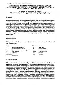
Fig. 1. Vertical and horizontal light planes in the 30° and 0° slope conditions. (a) Shows the bench in the 30° slope configuration. A technical personnel observes the plane jet by testing the smoke generator Thermocouples (b) and heat fluxmeters (c) are fixed on a Syporex support (white rectangle) at X = 8 m on the bench.

at X = 1 m using alcohol; the fire spread to a distance of up to X = 7 m. A complete schematic of the experimental setup is shown in Fig. 2. The optical methods used to determine the flow velocity are presented below.

chemiluminescence imaging, which would provide the location of the reaction area with respect to the flow field as measured by the PIV device.). The remainder of this paper is organized as follows. Section 2 presents the experimental fire protocol implemented on the DESIRE bench and all experimental diagnostic settings: the PIV and heat measurement systems are described in this section. The results are presented in Section 3 and discussed in Section 4, while the conclusions are presented in the last section.

2.1. Specific features of PIV in present work We recall that Particle Image Velocimetry (PIV) generates first a couple of tomographic images by synchronizing a PIV camera with a double pulse laser. Then, the displacement of particles from the first to the second image is measured by a statistical method called intercorrelation. Finally, the velocity field is computed from this displacement observed over an inter-image time interval. The conditions for performing large-scale PIV for a spreading natural fire are reported in [17]. Here, we discuss the method used to adapt the PIV technique to a fire spreading across vegetal fuel when the fire bed is increased from a 1- to an 18-m2 sloped bed for a comparable fuel load. First, these conditions require the generation of PIV images with a larger field of view compared to the 1-m2 case, because the flame height and fire size are greater. Indeed, for the 1-m2 fires with 0° or 30° slope examined previously, the flame length did not exceed 0.43 m for a 0.4-kg/m2 fuel load [18]. In this study, an 18-m2 fuel bed was considered and the fuel load was increased by a factor two, from 0.4 to 0.8 kg/m2. Thus, the flames were expected to be considerably longer. The previous size of the PIV measurement area was 0.7 × 0.7 m2 [18]; in the present study, this area is increased to 2 (length) × 1.5 (height) m2. This increased size generates another difficulty regarding the performance of measurements in

2. Experimental facility and devices In June 2013, a series of fire experiments were conducted on the DESIRE bench at the Institut National de la Recherche Agronomique (INRA) laboratory (Fig. 1). The INRA facility is described in detail in [8,9,14]. The large-scale DESIRE bench is 10-m long and 3-m wide, and has an inclinable plate made of an insulator (Siporex) that can be set at angles within the 0–30° range. Furthermore, the edges of the combustion bench are surrounded by four rulers with 25-cm gradations. The fuel bed consisted of a 6-m-long and 3-m-wide excelsior bed (18 m2). The fuel bed depth was measured at three random locations per square meter. The surface-to-volume ratio and density of the fuel were 4730 m−1 and 780 kg/m3, respectively. A constant fuel load, fuel homogeneity, and fuel-bed bulk density were maintained during the experiments. Three fuel loads of 0.4, 0.6, and 0.8 kg/m2 were used for the entire set of experiments. The fuel samples were not conditioned in an oven before the fire tests and their moisture content was ∼10%, being consistent with previous experiments [9]. A fire line was ignited 185

Experimental Thermal and Fluid Science 92 (2018) 184–201

X. Silvani et al.

Fig. 2. Scheme of the overall experiment.

a large-scale fire scenario. That is, for a given fuel load, these 18-m2 fires exhibit higher fireline intensity than that encountered in the 1-m2 case. They generate a stronger heat impact on their surroundings, both because of the high-heat smoke flows and a higher level of heat transfer via radiation. This level may reach up to 80 kW/m2 [9]. This behavior can cause irreversible damage to the expensive optical devices positioned adjacent to the fire, if the distance from the fire to optical setup is insufficient. Therefore, in this study, the positions of the laser sources and cameras were required to be increased significantly, from the approximately 2-m distance from the fire employed in [18] to a 6-m distance (Fig. 2). However, despite this precaution, measurement could not be performed for the most powerful experimental conditions, 0.8 kg/m2 at a 30° slope, in order to preserve the integrity of the PIV device and the measurement quality. Note that a safety distance for heat impact longer than 6 m could not be established in the experiment hall. Because of this change in the optics locations, it was necessary to adjust the cameras and lens systems to guarantee a pixel (px) resolution close to that provided by the 0.7 × 0.7 m2 PIV images presented in [18]. In particular, the PIV camera used in [18] (Hamamatsu C9300-

024, 2048 × 2048-px resolution, 12-bit dynamic range) offered a spatial resolution of 0.35 mm/px for a 1-m2 fire. In the experiment reported here, we used a ViewWorks PIV camera (resolution: 3280 × 2472 px, 12-bit dynamic range) to capture the Mie scattering signal from the vertical light plane. This camera combines a greater px resolution with a higher-bit dynamic range compared to the Hamamatsu device, allowing upgrading of the gradient contrast in the tomographic image. Further, the ViewWorks PIV camera uses a Nikon 50mm f2.8 lens coupled with an electro-mechanical shutter (EMS) to prevent flame and soot illumination in the second PIV image. It is important to note that the use of a liquid crystal shutter (LCS), which was recommended in previous works [17,18], was not technically possible for the ViewWork camera and Nikon 50-mm lens in this study, because of the modulation transfer function (MTF) on the LCS. Further, the flame and soot illumination control in the second PIV image is of weaker quality when the EMS is used compared to that obtained with the LCS; this is because the aperture intervals are longer with the EMS than those for the LCS, generating a longer exposure time to flame and soot illumination, which affects the contrast in the seed particle definition. Finally, the ultra-high definition of the ViewWork camera allows 186

Experimental Thermal and Fluid Science 92 (2018) 184–201

X. Silvani et al.

diagnostic for capturing the flame gradient in the light plane, one cannot accurately locate the position of the flame contour in the velocity measurement window. Therefore, because colored digital highdefinition (HD) video is easily available, we chose to observe the flame front using visible video data, by representing the position of the PIV window in each experiment.

a pixel resolution of 0.61 mm/px in a 2 × 1.5 m2 PIV measurement area for an 18-m2 fuel configuration. This resolution conveniently approaches the 0.35-mm/px setup obtained with the Hamatatsu camera used for the previous 0.7 × 0.7-m2 PIV measurement area for 1-m2 fires. Finally, the upgrade in pixel resolution is expected to compensate the lower quality of the EMS. Beyond, our experience indicates that a varied set of optical components is often required to achieve the optimal setup for such experiments, as there is no standard configuration for PIV under fire conditions. In addition, there is no trivial method of adapting the view system of the intensified charge-coupled device (ICCD) camera (Roper Princeton Instruments IMAX2, 512 × 512-px resolution, 16-bit dynamic range) used in [18] to the configuration employed in this study. This device allows observation of the scalar field via the OH∗ chemiluminescence. However, in [18], the viewing area captured by the ICCD camera did not exceed 0.7 × 0.7 m2 when the camera was located 2 m from the burning fire. In the present configuration, the ICCD camera was required to be set at least 6 m from the fire; thus, the spatial resolution of the digital camera was divided by a factor of three. This limitation prevented us from considering the OH∗ chemiluminescence under the experimental conditions in this study. Further, despite the stronger radiative environment compared to the 1-m2 lab-scale fires, the signalto- noise ratio was not expected to be sufficiently good for measurements to be performed with the ICCD camera.

2.3. Particle intercorrelation method Usually, it is necessary to set the size of the interrogation windows in PIV measurements, and to set the intercorrelation algorithm. In addition, the possible overlap and the threshold of the possible gray-level filter must be set. The instantaneous velocity fields are then post-processed via different spatial filters and, eventually, interpolated. Under these conditions, computation of the instantaneous velocity fields in this study, which involved three different fuel loads at a scale increased by one order of magnitude over that reported in [18], was considerably more difficult and time-consuming than similar computations in previous works. Indeed, each fuel load and each slope case required adaptation of the entire set of previous parameters to provide optimally computed velocity fields. If the natural seeders of the flow are not in sufficient concentration, an effective seeding is therefore required in order to guarantee the production of tomographic images with the best possible texture i.e. the greatest spotted in the image. We recall that the term “seeding” stands for the presence of solid particles injected at low initial velocity in the flow for generating a regular image of light spots: the spots are formed by the Mie scattering of the incident laser light over these particles. Such images are required for efficient computation of the displacement of the inter-correlation peak in the velocity determination method. Indeed, we previously demonstrated that PIV in the open over a 50-m2 fire with no slope conditions is feasible [17]. However, because of the complex aerology acting under outdoor conditions, the PIV may be affected by the dispersion of the seeding particles far from the light plane. In the indoor conditions considered in this study, the preliminary tests convinced us that the seeding particles should be injected directly from the fuel bed in the light plane (Fig. 2). However, the acquisition of a good texture in the tomographic images in small-scale fire experiments conducted under indoor conditions also requires a seeding system [18]. A similar system was employed in [21], using Al2O3 particles. These previous fire-facing PIV experiments therefore informed us that a dedicated seeding system was also required in the large-scale indoor fire study conducted in this study. Therefore, a system consisting of copper tubes as long as the PIV measurement field, each having a 30-cm aperture, was used. A slow flow blew the particles through the fuel bed to ensure the highest possible uniformity in the seeding of each light plane. The seeding material is zirconium oxide (ZrO2), with 5 μm diameter because, thanks to their high fusion temperature (2700 K), these particles are not consumed into the flame. A smoke fog provided by a fog machine completes the seeding of the overall hall. Under these conditions, we were required to determine whether the artificial flows for seeding were intrusive as regards the considered fire configuration. That is, we examined whether they had a significant effect on the overall surrounding flow generated by the fire. To examine this possibility, particle jets with the lowest possible mass rate were established to promote both a lower-momentum impact on the fire flow and good tomographic image quality. In the vertical tomographic images obtained for the 0°- and 30°-slope conditions (Fig. 3), natural entrainment of the particle jets induced by the flame fronts from the emitting tubes were clearly observed, even far from the fire. The particle were naturally aspirated by the flow induced by the flame front, even several meters ahead of the fire. Therefore, the seeding had a negligible influence on the flame front dynamics. The behavior of the particle flow far away from the fire front are also in accordance with the complex fire-induced air inflows reported in other works [11]: furthermore, its change with the approaching fire provides new insight on

2.2. Light planes and optical devices A pulsed laser plane was generated in the vertical direction, normal to the bench and at its centre (Fig. 2). In this study, the orthogonal direction only was considered, because the main focus was the differences compared to the 1-m2 case [18], for which the normal velocity field only was measured. We also planned to investigate the flow parallel to the plate at the top of the vegetal fuel bed; however, these findings will be discussed in a future paper. We inform the reader of the existence of the second light plane here, because this plane affected the heat measurement system deployment. However, the PIV in the vertical direction only is presented and discussed in this paper. The laser source used in the vertical direction for this experiment was a Quantel doublepulse 2 × 200-mJ laser, which was centered on the 532-nm ray. In order to observe the dependence of the tomographic image texture on the fire configuration, we conserved the flow illumination from the downstream side of the fire for all fuel loads and slope conditions. The vertical PIV window size was 2 × 1.5 m2 and each laser pulse illuminated the fire for a 7-ns period. The inter-image time was set to 3 ms in the vertical direction under 0°-slope conditions and 2 ms under 30°slope conditions. The laser-pulse couple was generated at a 14-Hz frequency; thus, the velocity field measurements were performed at a rate of 7 fields per second. The overall fire spread was observed from the side view using a Guppy F080C digital visible camera (28 fps) with a resolution of 1032 × 778 px (previously used in [18]). This optical device allowed measurement of the rate of fire spread (RoS) and flame height. These features are the kinematic and geometrical quantities conventionally measured in fire science. They respectively contribute to qualitative evaluation of the fire strength and the fire intensity, as a greater RoS and a higher flame indicate a bigger fire, i.e., a larger radiant volume indicates a greater upwind flow or slope effect. Thus, their values are usually correlated with the fire heat release. In this study, the RoS and flame height were measured from the visible video data. All these quantities are reported in Table 1. The RoS spread was measured from the propagation of the flame base over the fuel bed, along the ray of the green light plane intercept on the vegetal fuel bed at the bed centre. Note that the RoS values were rounded to upper units for convenience. The flame height was defined as the length of the normal to the plate passing through the flame top. It is important to mention that, in the absence of an optical 187

Experimental Thermal and Fluid Science 92 (2018) 184–201

X. Silvani et al.

Table 1 Fuel bed and kinematic/geometric features of the flame front during the 5 experiments. Slope

Fuel load 400 g/m2 Fuel height:

600 g/m2 Fuel height:

800 g/m2 Fuel height:

0°

ROS: 14 mm/s Flame height: 0.57 ± 0.03 m

ROS: 23 mm/s Flame height: 1.13 ± 0.15 m

ROS: 32 mm/s Flame height: 1.25 ± 0.31 m

30°

ROS: 91 mm/s Ball flame height: 0.625–0.75 m Elongated flame h.: 1.02–1.39 m

ROS: 194 mm/s Ball flame height: 1.08–1.38 m Elongated flame h.: 1.63–2.38 m

Not possible [Critical heat release: hazard!!] [ROS too important for PIV]

Therefore, the first line of heat sensors was positioned at X = 8.25 m (Fig. 2). Second, to avoid this interaction with the light plane parallel to the plate generated at the top of the vegetal fuel bed (Fig. 2), it was necessary to position the parallelepiped supports of these sensors 20 cm above the insulator ground, where the fuel bed was spread. Thus, unlike the experiments reported in [9], measurements for this experiment could not be performed at the top of the vegetal fuel beds but, rather, 20 cm above the ground. The temperature and heat flux measurements were recorded using an Agilent data logger combined with a VT1419A multifunctional measurement card, as in [9]. The temperature accuracy was computed for a constant range ( ± 1 °C), being dependent on the gain and offset of the data logger. Note that, when used under the nominal conditions recommended by the manufacturer, the error relative to the temperature data acquisition does not exceed 10% of the radiative loss/gain error of the thermocouple mentioned above. The acquisition error relative to the HFM input was approximately ± 0.01%, yielding a data acquisition error of 0.02 kW/m2. The HFM error was usually dominated by the calibration error of the HFM under pure black body irradiance, as previously mentioned (3% of the responsivity, with a coverage factor of 2 for a 95% confidence interval, according to the Medtherm black body calibration report [25]). Furthermore, considering the time constants of the thermocouples and devices, a sampling rate of 10 Hz was chosen. We also considered the fluctuating contribution of the thermal signals. In this study, the robust statistical analysis presented in [15] could

the flow motion information that can be yielded by laser tomographic images.

2.4. Experimental protocol for heat measurement The experimental protocol for heat measurement was close to that previously used on the bench and detailed in [9]. The reader may refer to that publication for details concerning the heat sensors and data acquisition system. In Fig. 2, each heat measurement point is represented by a violet disc, with the points being numbered S1–S4. Each point combines a heat fluxmeter (HFM; Medtherm Corporation) couple with a K-type thermocouple with a 250-µm-diameter grounded junction (50-µm wires). The HFM couple was formed using both total and radiative heat gauges. The radiative heat gauge differs from the total heat gauge in terms of the window placed in front of the sensitive element. In the radiative heat gauge, the spectrum transmitted by the sapphire window is 85% nominal from 0.15 to 5.0 µm; however, all convective effects are blocked. In other words, the radiative HFM is insensitive to heat convection. In the experiment conducted in this study, the use of a laser-based velocity measurement system for PIV required adaptation of the protocol used in [9]. First, heat measurements could not be performed at the upper edge of the vegetal fuel but, rather, at a distance of 1.25 m. In particular, we were required to avoid the intrusive effects of the solid instruments in the PIV window, as well as any possible reflection of intense laser light on these devices (sensors, wires, and cables).

Fig. 3. Fire-induced inflow effect on seeding jets at 0° (top)/30° (bottom) slope in the 0.4 kg/m2 experiments. The white arrow illustrates direction and sense of the particle flow. In both conditions, it follows the flow motion of air entrained by the fire.

188

Experimental Thermal and Fluid Science 92 (2018) 184–201

X. Silvani et al.

Fig. 4a. Heat measurement: time evolutions of heat quantities under 0° slope conditions: Temperature (left) and heat fluxes (right) for 0.4 kg/m2 (top), 0.6 kg/m2 (centre) and 0.8 kg/m2 (bottom).

convective heat transfer, with the direction of the transfer being indicated by the sign of ΔHFM. Thus, if ΔHFM = total HFM – radiant HFM is positive, the convective heat transfer warms the total heat sensor. In contrast, if it is negative, a cooling process of the sensor due to the surrounding flow is indicated. However, no calibration method for the total HFM facing the heat convection has been developed (as reported in the Round Robin Study for Gardon and Schmidt-Boelter Medtherm© gauges [4] and the International Standard Organisation report on HFMs [25]). That is, the HFMs are calibrated for pure black body irradiance only. Therefore, Gardon and Schmidt-Boelter Medtherm© gauges should not be used to quantitatively measure the convective heat flux.

not be performed, because of the limited number of replicates (only 3 replicates in each case). It was necessary to investigate the fluctuating features of the thermal data using a different approach, as demonstrated in the previous experiment conducted on the DESIRE bench [9]. Thus, the temperature and heat flux time curves were filtered using a 4th-order Butterworth filter in order to split the signal into long-term and fluctuating parts [5]. The selected cut-off frequency was 0.5 Hz, which was one order of magnitude smaller than the Nyquist frequency. Finally, the data logger recording the heat data was synchronized with the optical systems on the same reference clock to form a unique time base. In the fire science community, it is assumed that the difference between the total and radiant heat flux signals ΔHFM indicates the 189

Experimental Thermal and Fluid Science 92 (2018) 184–201

X. Silvani et al.

3. Results

The sensor position justifies the reasoning that the amplitude of each heat quantity in the present work cannot be directly compared to the findings of previous studies. However, qualitatively, the behavior of each quantity complies with previous experiments. An increase in temperature to a peak value as the fire approached can be immediately observed. For each thermocouple, the temperatures reached a maximum value when the flame front reached the end of the plot at X = 7 m. For sensor S2, located at the centre of the plot, the temperature ranged from 36.7 °C under the 0.4-kg/m2 fuel load and zero-slope conditions (Fig. 4a) to 420 °C under the 0.6-g/m2 fuel load and 30°slope conditions (Fig. 4b). Therefore, there was no direct flame contact on the sensors, as a temperature of approximately 800 +/− 300 °C is expected in the case of contact for these kinds of fire experiments [9]. The heat flux measurement results follow the same evolutionary trend, with maximum values of 3.5 and 70 kW/m2 being obtained for the 0.4kg/m2 fuel load and zero-slope conditions and the 0.6-g/m2 fuel load and 30°-slope conditions, respectively. One can also understand why the case of the 0.8-kg/m2 fuel load under a 30° slope could not be implemented on the bench, as heat fluxes greater than 70 kW/m2 damage the fragile optical devices and laser sources. For horizontal fire (Fig. 4a), the radiant heat flux (FR) and the total heat flux (FT) profiles are almost equal. Globally, these results confirm the findings for heat measurements performed in previous bench tests [8,9,14]. Under zero-slope conditions, the heat radiation strongly dominates the heat transfer process ahead of the flame front. [16] suggested that a turbulent diffusion process is associated with the natural convection close to the flame front. In the experiments conducted in this study (Fig. 4), FT and FR were identical for sensor S2, whereas FR was greater than FT for sensor S3. The FT results also exhibited negative values. Thus, it was necessary to detail the relative response of the total heat sensor to the expanded uncertainty. The HFM values were qualified against pure irradiance with 3% responsivity and a coverage factor of 2. For instance, when the recorded value was 0.5 kW/m2, there was a 95% probability that the measured value was within the [0.47; 0.53]-kW/m2 interval. Before reaching the maximum heat flux, the total HFM measured value and the radiant HFM measured value fell within the same 0.06-kW/m2-wide confidence interval under the zero-slope condition. In such a case, we cannot determine the sign of the difference between the total and radiant HFM signals (ΔHFM), which scales to approximately 0.5 kW/m2 (i.e., to approximately the size of the confidence interval). Therefore, we believe that the sign of ΔHFM cannot be interpreted as a clear indication of the cooling or warming convective mechanism of the vegetation ahead of the flame front (Fig. 4a; right, from top to bottom). Higher-accuracy HFMs are required in order to capture this subtle effect, which occurs more than a flame-length from the fire. Fortunately, the present work provides new insight on this mechanism via the PIV. In the case of the 30° slope, where the flames were elongated in the direction of the plate and where a hot smoke flow was generated, a significant positive ΔHFM appeared (Fig. 4b). For instance, for sensor S2 at t = 30 s, ΔHFM was greater than 3 kW/2m when the size of the 95% confidence interval was approximately 2 kW/m2. Therefore, in that case, the difference between the FR and FT was clearly positive and greater than the breadth of the HFM confidence interval. Thus, a positive convective flux was observed to flow to the HFMs located 1.25 m from the upper edge of the vegetal fuel bed. Further, the flame did not enter into prolonged contact with the sensor, because the temperature did not exceed 500 °C, even for the heaviest load (0.6 kg/m2). Further, the gas temperature reached 450 °C, illustrating that the gaseous environment of the sensor was considerably hotter than that in the 0°slope case. Therefore, it is likely that a hot flow was responsible for the convective heat flux, which warmed the FT.

3.1. Rate of fire spread (RoS), flame geometry, and heat quantities In [9], RoS was measured from a top view of the bench, by tracking the longitudinal position of the fire head versus time in a 0.4 kg/m2 scenario. In this case, the RoS was estimated by fitting a linear regression of these data. Because steady correlation factors (R2) were greater than 0.99, we concluded to a quasi-steady state of the fire spread. In the present work, it is estimated from the side view, as the velocity for a 1 m long displacement. The results for the RoS (and flame geometry) are listed in Table 1. The RoS increases with both the fuel load at a given slope angle and the slope angle, matching the values measured in [9] with another method. Furthermore, at 30° slope and a 0.6-kg/m2 fuel load, the RoS was up to 194 mm/s, which is comparable to that observed in fire experiments conducted under outdoor conditions and over large plots (e.g., experiment 4 in [13], all experiments in [23], S13 in [26]). Under zero-slope conditions, the flame front adopted a U-shape and the flame height was taken as the average value of 50 instantaneous flame-height measurements from the images acquired by the visible video camera. These values can be considered as statistically homogeneous around the averaged value with the root mean square (RMS) reported in Table 1. However, under 30°-slope conditions, this “statistical homogeneity” is no longer guaranteed, as the flame fluctuated strongly between two extreme shapes during the spread. A “spherical flame” configuration describes a situation where the fire head is compact at the tip of the V- shape fire, forming a “ball”. An “elongated flame” configuration described a flame elongated along the longitudinal direction of the inclined plate, forming an angle with the inclined fuel bed. In both cases, the fire head propagates in the light plane, at the centre of the bench. Under 0°-slope conditions, the flame height ranged from 0.57 to 1.25 m for fuel loads of 0.4 and 0.8 kg/m2, respectively. The flame height increased with the fuel load and, also, with the slope. Indeed, under 30°-upslope conditions and a 0.6-kg/m2 fuel load, the flame height increased up to 2.38 m in the elongated flame configuration. This value illustrates how the increase in the heat impact distance in response to increases in the fuel-load and slope conditions generates a safety problem. The time evolutions of the heat quantities, i.e., the temperature and heat flux, are shown in Figs. 4a and 4b for a 0° and a 30° slope, respectively. Each plot associates a visible video image (Fig. 5, left) and its corresponding velocity field (Fig. 5, right). The position of the PIV window is represented by a red rectangle in each visible digital image of the fire. In heat plots (Fig. 4), a green (resp. blue) vertical line indicates the instant when the flame base enters (resp. leaves) the PIV window in the visible image. This provides a relatively accurate indication of the flame position in the velocity field, but does not provide the plot of the flame intercept in the light plane. Data from S1 and S4 (Fig. 1) are not provided so as to facilitate a clearer reading of the results; note that the S1 data are symmetrical to those of the S3 sensor and the levels of the S4 sensor data are consistently lower than the other signals. Thus, these supplementary measurements do not provide any further comprehensive information about the physics investigated here. The measurements provided in this paper are consistent with experimental heat measurements reported in the literature [8,15,16], but some significant differences exist. First, in [15,16], the measurements were intrusive, i.e., the spreading fire passed through the sensor location. Contact between the fire and sensors was also observed in [9]. In the present study, no contact between the sensors and fire was allowed, as the metallic supporting rods could induce perturbation of the downwind flow, which is observed in the PIV measurement area. Recall that this is the reason why the heat sensors were installed at X = 8.25 m, i.e., approximately 2 m from the upper edge of the PIV window (X = 4.25–6.25 m at 0° slope and X = 4.50–6.50 m at 30° slope; Fig. 2).

3.2. Velocity field normal to fire plane under 0°-slope condition Obviously, the primary new insight provided by the PIV under these 190

Experimental Thermal and Fluid Science 92 (2018) 184–201

X. Silvani et al.

Fig. 4b. Heat measurement: time evolutions of heat quantities under 30° slope conditions: Temperature (left) and heat fluxes (right) for 0.4 kg/m2 (top) and 0.6 kg/m2 (bottom) – Red (resp.blue) down arrow indicate local maxima (resp. inflexion) of total heat fluxes. (For interpretation of the references to colour in this figure legend, the reader is referred to the web version of this article.)

conditions concerns the velocity field in the flame front and its surroundings. Under 0°-slope conditions, the flame front spread as a single line that was slightly curved near the edges of the plot. This front featured oscillating vertical buoyant flames and exhibited a U-shape [8,9,14]. Therefore, the velocity field resulting from a buoyant mixing layer was observed, which was driven by the natural elevation of the reactive hot gases in the cooler atmosphere through a gas-phase combustion process. The corresponding velocity field is represented in Fig. 5. To help the reader locate the flame in the velocity field, even roughly, we used tiny black vertical lines to indicate the X-positions of the flame heads in the PIV images. Each of these plots contain regions in which the velocity vectors are computed, along with smaller regions in which they cannot be calculated. The latter are “sink” regions, i.e., regions in which the particle concentration is insufficient to provide relevant velocity data. Significant attenuation of the laser was also observed after the fire, reducing the Mie scattering intensity recorded by the camera. The maximum velocity increased with increasing fuel load. Thus, the height at which this maximum was located also increased. Regarding the streamlines of the velocity fields under the 0°-slope condition (Fig. 5), the structure of a convective flow of fresh air toward the hotter regions of the fire was apparent. On the right side of each image in Fig. 5 and despite the presence of sink regions, the flow is clearly oriented from the surroundings toward the vertical buoyant convective column. Further, the flow behind the fire (Fig. 5, (left) was hotter than the region ahead, because it was also formed by hot smoke flows

proceeding from the fuel combustion process. This indicates that fewer sink zones with unresolved velocity vectors were located behind the fire than in front. Note that smoke strongly increases the seeding of the light sheet in the particles and, therefore, the resulting PIV resolution. This behavior was particularly visible when the fire was about to leave the PIV window (Fig. 5). Under 0°-slope conditions, the PIV allows the computation of several new quantities related to the velocity field. Thus, we examined whether the PIV could provide a statistical decomposition of the field in order to support the modeling strategies. At these scales and under real conditions, the fire is a turbulent flow. Computational fluid dynamics approaches regard this turbulent flow as resulting from mass, momentum, and energy balances. In this description, each quantity is decomposed into an “averaged” part and a fluctuating part in Reynolds or Favre averaging [27–32]. Each conservative field, i.e., the mass, momentum, and energy, is also split according to the large eddy simulation approach [33,34], through a spatially filtered and sub-grid scale component. Fig. 6 presents an attempt to produce time-averaged velocity fields for each load, based on 10 fields roughly acquired from either side of the central position of the mixing layer in the PIV window. The 10 consecutive velocity fields were obtained within a 1.4-s period, because 7 image couples are generated each second for a 14-Hz PIV. During this time interval (1.4 s), with respective ROS values of 14, 23, and 32 mm/s (Table 1, first line), the displacements of the naturally convective mixing layer due to the flame were 19.6, 32.2, and 44.8 mm for the 0.4-, 0.6-, and 0.8-kg/m2 experiments, respectively. Hence, these

191

Experimental Thermal and Fluid Science 92 (2018) 184–201

X. Silvani et al.

Fig. 5a. Vertical velocity field in 0° slope and 0.4 kg/m2 conditions (t = 103 s (top) – 158 s (centre) – 181 s (bottom)) White (resp.black) line set the X position of the fire heat in the visible (resp.velocity) image.

corresponds to a negligible error due to the fire spread. We then considered whether the fire can be observed as statistically stationary during the 1.4-s period for which averaging was performed. Here, the vertical momentum of the gases increased with increased fuel load, as

displacements were small in comparison with the length of the vertical mixing layer. These values also correspond to 0.98, 1.61, and 2.24% of the 2-m PIV window length, respectively. Ultimately, this means that averaging 10 velocity fields along these small displacements 192

Experimental Thermal and Fluid Science 92 (2018) 184–201

X. Silvani et al.

Fig. 5b. Vertical velocity field in 0° slope and 0.6 kg/m2 conditions (t = 72 s (top) – 121 s (centre) – 135 s (bottom)).

Overall, stronger velocity maxima and fluctuations and a departure from the assumption of fire stationarity during the averaging time interval are the consequences of a greater fuel load. The above attempt to produce the statistical moments of the velocity field so as to adhere to fire turbulence modeling approaches indicates a limitation of the present PIV. However, even if the results are not entirely satisfying, the present experiment indicates that a significant enhancement of the data

indicated by stronger velocity maxima. This increase of the vertical momentum also generated stronger local fluctuations. One can therefore conclude that the fuel load increase generated increasingly strong fluctuations; thus, it became increasingly difficult to smooth these fluctuations in the average profile. Hence, the stationary feature of the flow was weakened and the velocity gradients were stronger. The corresponding time-averaged fields are presented in Fig. 6. 193

Experimental Thermal and Fluid Science 92 (2018) 184–201

X. Silvani et al.

Fig. 5c. Vertical velocity field in 0° slope and 0.8 kg/m2 conditions (t = 52 s (top) – 80 s (centre) – 99 s (bottom)).

varied between two extreme topologies, namely “spherical” and “elongated” flames. In both cases, the fire head propagates in the light plane at the centre of the bench. Spherical and elongated flames are shown in Figs. 7a and 7b, respectively, for a fuel load of 0.4 kg/m2 and in Figs. 8a and 8b, respectively, for a fuel load of 0.6 kg/m2. In the 30°-slope fire experiments, we considered the velocity fields for both the observed spherical and elongated flame configurations. In

can be expected for a faster PIV setup in future experiments. 3.3. Velocity field under 30°-slope condition Under sloped conditions, there is no statistical homogeneity. Indeed, during fire spread for the 30° slope, we observed that the flame front exhibited a V-shape and the fire head in the light plane strongly 194

Experimental Thermal and Fluid Science 92 (2018) 184–201

X. Silvani et al.

conducted on the DESIRE bench [8,9,14] have shown that flame elongation at the forefront of the fire coincides with the ejection of strong flaming helical whirls, which roll upwards along the flanks of the V-shaped flame under 30°-slope conditions. A photograph obtained using a 500-image/s camera focused on the flame front flank illustrates the detailed structures of these whirls (Fig. 9), which contribute to the dynamics of the flame head elongation. For the 30°-slope case, the velocity field was more or less tilted with regard to the fire propagation plane. This tilt resulted from the combination of both the vertical impulse of the hot flow in the colder atmosphere and the fire-induced draft behind the flame front, which drew fresh air along the inclinable bench. It is apparent that, in every configuration, the velocity field upwind of the flame front was well resolved. The mechanical stirring induced by the sloped fire aided the homogeneous mixing of the seeding particles behind the flame front, thereby facilitating a higher-accuracy velocity computation. It is apparent that, despite the 3D structure of the V-shaped fire under the 30°slope conditions, the fire head spread inside the light plane. Therefore, although the visible video of the fire and the planar PIV pictures could not be matched, the global position of this flame head in the PIV window could be qualitatively used to appreciate the sloped-fire effect on the velocity field. The maximum velocity values increased significantly with increasing slope. During the elongated flame phase, the maximum velocity also increased with the fuel load, ranging from 4.5 to 5.5 m/s for a 0.4-kg/m2 load to more than 7.5 m/s in the 0.6-kg/m2 case (Fig. 7b). One can reasonably assume that this increase resulted from the stronger momentum provided by the heaviest fuel load. Indeed, Fig. 4b illustrates that the 0.6-kg/m2 fuel-load case yielded stronger heat fluxes. Table 1 lists the largest RoS values. Both indicate a stronger heat release, which generated greater vertical impulses of hot gases in the colder atmosphere, along with stirrer-induced upwind flow with stronger transversal velocity gradients (Fig. 7b). These maxima seem to have been located at the upper edge of the elongated flame, where hot gases were ejected. However, it is considerably more difficult to assess their location for the spherical flame configuration. This finding again indicates the need for the development of an optical diagnostic method for the scalar field temperature or chemical radicals, to allow their observation in the measurement window in conjunction with the computed velocity field. The slope effect on the heat transfer ahead of the flame front has been discussed in previous studies conducted on both the intermediate [9,11] and field scales [23]. In those cases, a significant convective warming flow was detected by the total HFM. That measurement result indicates an actual change in the flow motion ahead of the fire in comparison with the behavior for the 0° slope described in the previous subsection. Indeed, in the 30°-slope fire, fresh air was no longer aspirated from the immediate surroundings toward the flame front and entrained in a vertical buoyant layer. The streamlines illustrate that the flow traveled from the fire to the region ahead, carrying hot gases towards the heat sensor and promoting convective warming of these regions. This is consistent with the positive convective heat transfer detected by the HFMs on S2, i.e., at the centre of the plot facing the periodically elongated flame head. Indeed, the positive value of ΔHFM at the S2 location confirms that the air flow on S2 was hotter than the surrounding air. In Figs. 7b and 8b, one can clearly observe the orientation of the streamlines ahead of the flame front. Thus, the PIV here elucidates a mechanism that was detected by analog sensors throughout the past decade, but for which a fine explanation was lacking. That is, the fresh air aspirated by the fire and the plume from behind and way ahead is warmed in the fire and transports heat near ahead. This behavior was only detected but not measured by the differential heat flux device (because the difference between FT and FR was positive). The length scales corresponding to “way ahead” and “near ahead” must still be identified.

Fig. 6. Time average velocity field in 0° slope condition (0.4 kg/m2 - top- 0.6 kg/m2 -centre- 0.8 kg/m2 -bottom).

Figs. 7 and 8, the visible video images of the flames obtained for the first laser shots of each PIV couple are shown along with the corresponding velocity field for each case. Previous fire experiments 195

Experimental Thermal and Fluid Science 92 (2018) 184–201

X. Silvani et al.

Fig. 7a. Vertical velocity field in 30° slope and 0.4 kg/m2 conditions – ball-like fire head (X location of the fire head in meters - time in seconds) from top to bottom: (4.69 m; 24 s) -(5.24 m; 26.4 s)- (5.6 m; 30.1 s).

front and the air flowing: as a consequence, the experimental design of a PIV protocol for outdoor fire involved powered laser sources, emitting in the visible (green) and a dedicated seeding system for avoiding the seeding particles dispersion far away from the light plane due to local air flow. If electrical alimentation of these different complex devices (laser source, camera and seeding systems) as their deployment is easier in an indoor hall, the experimental data in an 18 m2 indoor fire with flame height greater than 2.5 m remains reliable regarding larger outdoor fires. Indeed, the heat fluxes measured over the inclinable bench [9,22] are close to the ones measured in the field [3,5,10,12,13,23,24]. In another words, if the fire scales over the inclinable bench are not the real ones, they remain more realistic than smaller ones, regarding the

4. Discussion Fire is a scale dependent process [35]: the scale of the present experiments must first be discussed in order to appreciate the potential of these considering larger ones that have more practical importance. Let us discuss first the place of the present results in a broader conceptual context: the ambition of fire experiments is the measurement of coupled quantities involved in the conservation of mass, momentum and energy over time. PIV and HFMs allow to gain simultaneously the velocity field and the heat flux during a fire. In this framework, possibilities and limitations are investigated here. Indeed, previous work [17] showed that PIV measurements on natural fire was possible in the open, but suffering from light extinction across the flame 196

Experimental Thermal and Fluid Science 92 (2018) 184–201

X. Silvani et al.

Fig. 7b. Vertical velocity field in 30° slope and 0.4 kg/m2 conditions – elongated fire head (xfire;t) from top to bottom: (5.1 m; 26.3 s) -(5.6 m;29.6 s)- (6.18 m; 30.2 s).

especially, computational fluid dynamics strategies on a similar scale. Indeed, under 0°-slope conditions, the experimental results exhibit an original relationship between the velocity field and heat radiation ahead of the fire. Under zero-slope conditions, the fire was structured as a vertical buoyant mixing layer and aspired the fresh air ahead. The streamlines from the PIV data indicate that this buoyant mixing layer generated convective cooling of the vegetation ahead of the vegetal fuel bed through this air entrainment. This is clear for every velocity field in the 0° case. However, the HFM sensitivity was insufficient for clear detection of this convective cooling of the region ahead of the fire, because the order of magnitude of ΔHFM scaled to the size of the confidence interval. This limitation indicates the need for enhanced HFM accuracy and enhanced temporal resolution of the analog data gained on the

heat flux emitted in these indoor experiments. Indoor conditions make the use of the PIV possible, in safer and reusable conditions when outdoor ones only make the PIV feasible with no guarantee of reliable results. In a close future, the use of PIV versus a large scale fire in outdoor conditions would be technically possible with higher quality results once the dispersion of the seeding particles and the effect of light extinction through the fire front will be solved in the open. In this context, the present results mainly illustrate the new insights into fire physics provided by the combined use of optical diagnostics for velocity measurement and analog diagnostics for heat measurement. We can now provide synchronized velocity and heat data from a largescale inclinable fire bench, with the effect of the slope on these data being incorporated. This is a pioneering feature of our experimental work, which has immediate implications for fire modeling and, 197

Experimental Thermal and Fluid Science 92 (2018) 184–201

X. Silvani et al.

Fig. 8a. Vertical velocity field in 30° slope and 0.6 kg/m2 conditions – ball-fire head (xfire;t) from top to bottom: (5.05; 20.9 s) -(5.24 m;22.8 s)- (5.97 m; 25.5 s).

while considering the extreme topology of the fire head. Furthermore, regarding the time evolution of the heat data, the relationship between the local variations of the temperature and heat fluxes, the instantaneous flame topology, and the velocity field could be considered. For instance, three local maxima of the total heat fluxes on sensor 2 were particularly visible on the heat flux plot obtained under the 0.4kg/m2 fuel load (Fig. 5b, right; red arrow). These maxima were less apparent in the 0.6-kg/m2 case, where their local inflexions were almost undetectable (Fig. 5b, right; blue downward-pointing arrows). This damping of the local total HFM in the 0.6-kg/m2 case was due to a faster fire spread and a stronger overall amount of heat flux. As a result, the local maxima in the 0.6 kg/m2 had a weaker amplitude with regard

digital recorder. An overall increase in the measurement accuracy would allow these fine transport phenomena to be captured ahead of the flame front for 0°-slope experiments. Furthermore, the need to produce a converged statistical velocity field indicates the necessity of advancing the PIV system towards higher frequencies. This development requires establishment of an analog and optical measurement system that is faster overall, the design of which could be planned for future experiments. The contributions of the experiments conducted under 30°-slope conditions are also valuable. The statistically non-homogeneous nature of the flow rendered the addition of average-based velocity profiles impossible in this case; however, we could measure the velocity fields 198

Experimental Thermal and Fluid Science 92 (2018) 184–201

X. Silvani et al.

Fig. 8b. Vertical velocity field in 30° slope and 0.6 kg/m2 conditions – elongated- fire head (xfire;t) from top to bottom: (4.6 m; 18.2 s) -(5.24 m; 24.9 s)- (6.09 m; 26.5 s).

to this overall level (70 kW/m2). Regardless, the local maxima are indicated by downward-pointing arrows on the FT2 curves in the corresponding parts of Fig. 5b. If we focus on the 0.4-kg/m2 sloped scenario, for instance, Fig. 4b shows that the local maxima of the total heat fluxes were reached at t = 23.45, 26.75, and 27.95 s. Each of these instants coincides with a flame elongation observed for the sloped fire in the image sequence captured by the Guppy digital video camera (Fig. 10). Thus, the local peaks of the total HFMs resulted from elongation of the flame in the sloped configuration. These local maxima of the heat fluxes contributed significantly to the overall spread and heat budget [5]. Unfortunately, only the first flame elongation image with local HFM maxima coincides

with a PIV computation. The last two images are not synchronized with the laser pulse. Therefore, only the velocity field relative to the first local HMF maximum could be computed. However, the present work demonstrates that the combination of heat flux and PIV measurements is valuable as regards investigation of the fine heat transfer due to largescale structures in a complex reactive flow and on an intermediate fire scale. One can therefore predict that upgrading the present setup will facilitate investigation of this phenomenon on shorter time scales. Thus, considerable improvements can be expected for future experiments with higher sample-rate measurement systems than those used here. For instance, Fig. 9 illustrates the level of detail we can expect from a 500-Hz data acquisition. Furthermore, under sloped conditions, the 199

Experimental Thermal and Fluid Science 92 (2018) 184–201

X. Silvani et al.

Fig. 9. Digital images of fire whirls and fire head at 200 frames per seconds: successive photographs of a fire whirl rolling along fire flank up to the fire head (time interval: 20 ms).

bench size limits the observation period for the fire spread. A larger PIV window would facilitate superior understanding of the fire dynamics under sloped conditions. The study also reveals the difficulties and limitations encountered when performing PIV during a fire spread on this scale. The first limitation concerns the damping of the light intensity by the gaseous reacting medium. That is, the sink regions observed ahead of the flame front in certain PIV images are regions from which the particles were absent or where the light scattering was insufficient for particle tracking. In particular, consideration of Figs. 5–8 indicates that the experiments suffer from a global lack of illumination ahead of the flame front (on the right side of the computed velocity field). This was due to the local damping up to extinction of the incident pulsed light, as a result of its absorption by the flame, the soot filaments, and the smoke. A possible solution to this problem is the use of a double laser plane yielding greater illumination of the flame front both upwind and downwind, simultaneously. However, this change would significantly increase the cost of the overall experiment and would necessitate adjustment of the heat sensor position downwind to a second laser source. The second limitation concerns the difficulty in providing a non-intrusive diagnostic of the scalar field, for correlation with the velocity fields.

5. Conclusion The present paper reports on the combined use of heat flux and temperature measurements coupled with a PIV system to examine the velocity field during the spread of an 18-m2 natural fire under zeroslope and 30°-upslope conditions. This study extended the results previously obtained at lab scale to an intermediate scale, in which the larger fire approaches real outdoor conditions in terms of rate of spread, flame size, and heat flux levels (0.6 kg/m2 at 30° slope). The first set of heat/velocity measurements were produced, which are valuable for an improved understanding of the fire physics. At 0° slope, the flow of air entrained from the surroundings in the buoyant mixing layer due to the fire was captured by the PIV, despite uncertainty in the heat flux measurement. At 30° slope, the positive convective transfer from the fire to the region ahead was clearly observed by both the analog and optical systems; the flow structure was captured by the PIV device and the difference between the total and radiant heat fluxes measured by the thermal device was unambiguously positive. At 0° slope, some firstorder statistics of the velocity field were produced when fire steady state could be assumed. At 30° slope, the effects of flame elongations on the heat transfer could also be qualified. In the future, an improved understanding of these two key conditions will be possible with an upgrade of the time resolution and the spatial accuracy of both measurement systems. Finally, some additional limitations exist. Specifically, simultaneous measurement of the scalar field in the PIV windows (the OH∗ radical or temperature field) with chemiluminescence or PLIF systems is not trivial. Further, it does not seem possible at present to export the coupled

Fig. 10. Photographs of the flame front in 0.4 kg/m2/30° slope conditions at the nearest instant from 23.45 s, 26.75 s and 27.95 s These instants of capturing an elongated flame head coincide with time of local peaks on the total heat flux and reported by the red down arrows in Fig. 4b right. (For interpretation of the references to colour in this figure legend, the reader is referred to the web version of this article.)

200

Experimental Thermal and Fluid Science 92 (2018) 184–201

X. Silvani et al.

diagnostics setup used in this study to real fire scenarios [22]. First, the use of a powerful laser source in the open requires a guarantee of absolute eye safety for the entire local population, beyond the staff involved in the experiment. Second, further mechanical adaptations of the optical tools, i.e., the laser sources and digital cameras, are necessary, and the need for an electrical energy supply requires that the experiments are conducted near closed infrastructures. Based on these requirements, it can be stated that velocity-field investigation using PIV in a real “ad hoc” outdoor fire scenario, i.e., far away from any infrastructure, cannot yet be performed.

[12]

[13] [14] [15]

[16]

Acknowledgements [17]

The study was performed in the frame of the CORSiCA project, a Corsica Island FeDER funded project for studying the natural hazards in the Western Mediterranean (http://corsica.obs-mip.fr/). This work resulted from the collaboration of French public laboratories under INRA and the Centre National de le Recherche Scientifique (CNRS) with a private research and development (R&D) company with expertise in optical diagnostics (R&D Vision). The research was supported by the Collectivité Territoriale de Corse and the European Union. The authors gratefully thank Monsieur Antoine Pieri for valuable technical support during the experiments. They also thank Messieurs Joel Maréchal and Denis Portier for their assistance.

[18]

[19]

[20] [21]

[22] [23]

References

[24]

[1] F. Morandini, P.A. Santoni, J.H. Balbi, The contribution of radiant heat transfer to laboratory-scale fire spread under the influences of wind and slope, Fire Saf. J. 36 (2001) 519–543. [2] R. Bryant, C. Womeldorf, E. Johnsson, T. Ohlemiller, Radiative heat flux measurement uncertainty, Fire Mater. 27 (2003) 209–222. [3] F. Morandini, X. Silvani, L. Rossi, P.-A. Santoni, A. Simeoni, J.-H. Balbi, J. Louis Rossi, T. Marcelli, Fire spread experiment across Mediterranean shrub: Influence of wind on flame front properties, Fire Saf. J. 41 (2006) 229–235. [4] W.M. Pitts, A.V. Murthy, J.L. de Ris, J.-R. Filtz, K. Nygård, D. Smith, I. Wetterlund, Round robin study of total heat flux gauge calibration at fire laboratories, Fire Saf. J. 41 (2006) 459–475. [5] X. Silvani, F. Morandini, J.-F. Muzy, Wildfire spread experiments: Fluctuations in thermal measurements, Int. Commun. Heat Mass Transfer 36 (2009) 887–892. [6] D. Frankman, B.W. Webb, B.W. Butler, Time-resolved radiation and convection heat transfer in combusting discontinuous fuel beds, Combust. Sci. Technol. 182 (2010) 1391–1412. [7] W.R. Anderson, E.A. Catchpole, B.W. Butler, Convective heat transfer in fire spread through fine fuel beds, Int. J. Wildland Fire 19 (2010) 284–298. [8] J.L. Dupuy, J. Marechal, Slope effect on laboratory fire spread: contribution of radiation and convection to fuel bed pre-heating, Int. J. Wildland Fire (2010) in press. [9] X. Silvani, F. Morandini, J.-L. Dupuy, Effects of slope on fire spread observed through video images and multiple-point thermal measurements, Exp. Therm Fluid Sci. 41 (2012) 99–111. [10] D. Frankman, B.W. Webb, B.W. Butler, D. Jimenez, M. Harrington, The effect of sampling rate on interpretation of the temporal characteristics of radiative and convective heating in wildland flames, Int. J. Wildland Fire (2012). [11] N. Liu, J. Wu, H. Chen, L. Zhang, Z. Deng, K. Satoh, D.X. Viegas, J.R. Raposo,

[25] [26]

[27] [28]

[29] [30]

[31] [32] [33]

[34]

[35]

201

Upslope spread of a linear flame front over a pine needle fuel bed: The role of convection cooling, Proc. Combust. Inst. 35 (2015) 2691–2698. B.W. Butler, Experimental measurements of radiant heat fluxes from simulated wildfire flames, in: S.O.A. Foresters (Ed.), 12th International Conference on Fire and Forest Meteorology, Jekyll Island, Ga., 1993. X. Silvani, F. Morandini, Fire spread experiments in the field: temperature and heat fluxes measurements, Fire Saf. J. 44 (2009) 279–285. J.L. Dupuy, J. Maréchal, D. Portier, J.C. Valette, The effects of slope and fuel bed width on laboratory fire behavior, Int. J. Wildland Fire (2010) (in press). V.J.M. Mendes-Lopes J. M, A.J. M, Flame characteristics, temperature-time curves and rate of spread in fires propagating in a bed of Pinus Pinaster needles, Int. J. Wildland Fire, 12 (2003) 67. W. Anderson, E. Pastor, B. Butler, E. Catchpole, J.-L. Dupuy, P. Fernandes, M. Guijarro, J.-M. Mendes-Lopes, J. Ventura, Evaluating models to estimate flame characteristics for free-burning fires using laboratory and field data, For. Ecol. Manage. 234 (2006) S77. F. Morandini, X. Silvani, A. Susset, Feasibility of particle image velocimetry in vegetative fire spread experiments, Exp. Fluids 53 (2012) 237–244. F. Morandini, X. Silvani, D. Honoré, G. Boutin, A. Susset, R. Vernet, Slope effects on the fluid dynamics of a fire spreading across a fuel bed: PIV measurements and OH* chemiluminescence imaging, Exp. Fluids 55 (2014) 1–12. A. Koched, H. Pretrel, O. Vauquelin, L. Audouin, Experimental determination of the discharge flow coefficient at a doorway for fire induced flow in natural and mixed convection, Fire Mater. (2014) n/a–n/a. R. Bryant, The application of stereoscopic PIV to measure the flow of air into an enclosure containing a fire, Exp. Fluids 47 (2009) 295–308. J. Lozano, W. Tachajapong, D.R. Weise, S. Mahalingam, M. Princevac, Fluid dynamic structures in a fire environment observed in laboratory-scale experiments, Combust. Sci. Technol. 182 (2010) 858–878. X. Silvani, Metrology for Fire Experiments in Outdoor Conditions, Springer, London, Limited, 2013. F. Morandini, X. Silvani, Experimental investigation of the physical mechanisms governing the spread of wildfires, Int. J. Wildland Fire 19 (2010) 570–582. B.W. Butler, J. Cohen, D.J. Latham, R.D. Schuette, P. Sopko, K.S. Shannon, D. Jimenez, L.S. Bradshaw, Measurements of radiant emissive power and temperatures in crown fires, Can. J. For. Res. 34 (2004) 1577–1587. ISO, Fire tests — Calibration and use of heat flux meters — Parts 1-4, in: I.-I.O.o. Standardisation (Ed.) ISO 14934, ISO, 2014, pp. 16. X. Silvani, F. Morandini, E. Innocenti, S. Peres, Evaluation of a wireless sensor network with low cost and low energy consumption for fire detection and monitoring, Fire Technol. 51 (2014) 971–993. D. Morvan, J.L. Dupuy, Modeling of fire spread through a forest fuel bed using a multiphase formulation, Combust. Flame 127 (2001) 1981–1994. D. Morvan, J.L. Dupuy, Modeling the propagation of a wildfire through a Mediterranean shrub using a multiphase formulation, Combust. Flame 138 (2004) 199–210. J. Dupuy, D. Morvan, Numerical study of a crown fire spreading toward a fuel break using a multiphase physical model, Int. J. Wildland Fire 14 (2005) 141–151. D. Morvan, J.L. Dupuy, B. Porterie, M. Larini, Multiphase formulation applied to the modeling of fire spread through a forest fuel bed, Proc. Combust. Inst. 28 (2000) 2803–2809. B. Porterie, J.-L. Consalvi, J.-C. Loraud, F. Giroud, C. Picard, Dynamics of wildland fires and their impact on structures, Combust. Flame 149 (2007) 314–328. N. Sardoy, J.-L. Consalvi, B. Porterie, A.C. Fernandez-Pello, Modeling transport and combustion of firebrands from burning trees, Combust. Flame 150 (2007) 151–169. Y. Xin, J.P. Gore, K.B. McGrattan, R.G. Rehm, H.R. Baum, Fire dynamics simulation of a turbulent buoyant flame using a mixture-fraction-based combustion model, Combust. Flame 141 (2005) 329–335. W.E. Mell, S.L. Manzello, A. Maranghides, D. Butry, R.G. Rehm, The wildland–urban interface fire problem – current approaches and research needs, Int. J. Wildland Fire 19 (2010) 238–251. W.M. Pitts, Wind effects on fires, Prog. Energy Combust. Sci. 17 (1991) 83–134.