Media Segmentation using Self-Similarity Decomposition - fxpal

Media Segmentation using Self-Similarity Decomposition Jonathan T. Foote and Matthew L. Cooper FX Palo Alto Laboratory Palo Alto, CA 94304 USA {foote, cooper}@fxpal.com ABSTRACT We present a framework for analyzing the structure of digital media streams. Though our methods work for video, text, and audio, we concentrate on detecting the structure of digital music files. In the first step, spectral data is used to construct a similarity matrix calculated from inter-frame spectral similarity. The digital audio can be robustly segmented by correlating a kernel along the diagonal of the similarity matrix. Once segmented, spectral statistics of each segment are computed. In the second step, segments are clustered based on the selfsimilarity of their statistics. This reveals the structure of the digital music in a set of segment boundaries and labels. Finally, the music can be summarized by selecting clusters with repeated segments throughout the piece. The summaries can be customized for various applications based on the structure of the original music. Keywords: Digital media and audio processing, video and audio segmentation, music and audio summarization and thumbnails

1. INTRODUCTION Recently, decreasing storage costs, increasing bandwidth, improved compression technology, and peer-to-peer file sharing services have allowed many individuals to amass large collections of digital audio files. In a recent IpsosReid survey, more than half of consumers aged 25–34 have downloaded MP3 files onto home computers, storing on average more than 700 files.1 This is a substantial data management problem, and research and development of tools supporting music database management and music-related e-commerce has become increasingly active. Here we present an analytical framework to determine the structure of digital music streams. In particular, we demonstrate techniques for music segmentation, segment clustering, and summarization based on self-similarity analysis. Given structural characterizations of digital music files, appropriate summary excerpts and “retrieval proxies” can help to automatically organize personal or commercial music collections. Our methods depend on the analysis of a similarity matrix.2, 3 The matrix contains the results of all possible pairwise similarity comparisons between time windows in the digital stream. The matrix is a good way to visualize and characterize the structure in digital media streams. Throughout, the algorithms presented are unsupervised and contain minimal assumptions regarding the source stream. A key advantage here is that the data is effectively used to model itself. The framework is extremely general, and should work on any ordered media such as video or text as well as audio. In particular, we have demonstrated results on segmenting both speech audio4 and video streams5 as well as music. In this paper, Section 2 introduces similarity analysis and details how similarity matrices are constructed from audio. We then describe how the audio is segmented using kernel correlation. Section 3 describes how audio segments are clustered using a hierarchical similarity-based approach. The result is a comprehensive structural characterization of audio structure, including the locations and durations of repeated segments. As an example, the structure of a popular song is analyzed to determine repeated verses and refrains. The final Section 4 describes how the structure just determined can be used to automatically construct a representative music summary or “audio thumbnail”.

1

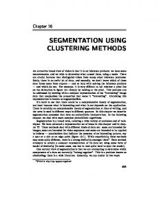
2. SIMILARITY ANALYSIS FOR MULTIMEDIA 2.1. Constructing the similarity matrix Self-similarity analysis is a non-parametric technique for studying the global structure of time-ordered streams. The first step is to parameterize the source audio. For this, we calculate spectral features from the short time Fourier transform (STFT) of 0.05 second non-overlapping windows in the source audio. We have also experimented with alternative parameterizations including Mel Frequency Cepstral Coefficients (MFCCs), and subspace representations computed using principal components analysis of spectrogram data. The window size may also be varied, though in our experience, robust audio analysis requires resolution on the order of 20 Hz. Here, the parameterization is optimized for analysis, rather than for compression, transmission, or reconstruction. The sole requirement is that similar source audio samples produce similar features. The analysis proceeds by comparing all pairwise combinations of audio windows using a quantitative similarity measure. Represent the B-dimensional spectral data computed for N windows of a digital audio file by the vectors {vi : i = 1, · · · , N } ⊂ IRB . Using a generic similarity measure, d : IRB × IRB → IR, we embed the resulting similarity data in a matrix, S as illustrated in the right panel of Figure 1. The elements of S are S(i, j) = d(vi , vj ) i, j = 1, · · · , N .

(1)

The time axis runs on the horizontal (left to right) and vertical (top to bottom) axes of S and along its main diagonal, where self-similarity is maximal. A common similarity measure is the cosine distance. Given vectors vi and vj representing the spectrograms for sample times i and j, respectively, dcos (vi , vj ) =

< vi , vj > . |vi ||vj |

(2)

There are many possible choices for the similarity measure including measures based on the Euclidean vector norm or non-negative exponential measures, such as dexp (vi , vj ) = exp (1 − dcos (vi , vj )) .

(3)

The right panel of Figure 1 shows a similarity matrix computed from the song “Wild Honey” by U2 using the cosine distance measure (see (2)) and low frequency spectrograms. Pixels are colored brighter with increasing similarity, so that segments of similar audio samples appear as bright squares along the main diagonal. Brighter rectangular regions off the main diagonal indicate similarity between segments. PCA/Spect Similarity

stream

i

start

j

end

20

start

0.8

40

D(i,j)

0.6 60 0.4

Time (sec)

80

i

100

0.2

120 0 140 −0.2 160 −0.4

180

similarity

200

matrix S

j

end

−0.6

220 −0.8 20

40

60

80

100 120 Time (sec)

140

160

180

200

220

Figure 1. The left panel depicts the embedding of the linear media into the two dimensional similarity matrix. The right panel shows a similarity matrix computed from the song “Wild Honey” by U2.

2

2.2. Audio Segmentation Segmentation is a crucial first step in many audio analysis approaches. The structure of S suggests a straightforward approach to segmentation.6 Consider a simple “song” having two successive notes of different pitch, for example a cuckoo call. When visualized, S for this example will exhibit a 2 × 2 checkerboard pattern. White squares on the diagonal correspond to the notes, which have high self-similarity; black squares on the off-diagonals correspond to regions of low cross-similarity. The instant when the notes change corresponds to the center of the checkerboard. More generally, the boundary between two coherent audio segments will also produce a checkerboard pattern. The two segments will exhibit high within-segment (self) similarity, producing adjacent square regions of high similarity along the main diagonal of S. The two segments will also produce rectangular regions of low between-segment (cross) similarity off the main diagonal. The boundary is the crux of this checkerboard pattern. To identify these patterns in S, we take a matched-filter approach. To detect segment boundaries in the audio, a Gaussian-tapered “checkerboard” kernel is correlated along the main diagonal of the similarity matrix. Peaks in the correlation indicate locally novel audio, thus we refer to the correlation as a novelty score. An example kernel appears in the left panel of Figure 2. The right panel shows the novelty score computed from the similarity matrix in Figure 1. Large peaks are detected in the resulting time-indexed correlation and labelled as segment boundaries.

2.3. Processing in the lag domain For segmentation, we need only calculate a diagonal strip of the similarity matrix with the width of the checkerˆ such that board kernel. Using a simple change of variables, we compute the N × K matrix S
 ˆ l) = S(i, i + l − K ) i = 1, · · · , N l = 1, · · · , K . S(i, (4) 2 ˆ in the “lag domain” to reduce computation and storage requirements, We refer to l as the lag, and compute S which can be substantial at high resolutions. Considering only the band of width K = 256 centered around the main diagonal reduces the computational requirements by over 96% for a three minute song sampled at 20 Hz. Kernel Correlation: Wild Honey

Gaussian Novelty Filter 1

0.9

0.02

0.8

0.015 0.7

0.01 0.6

0.005 0

0.5

−0.005 0.4

−0.01 −0.015

0.3

−0.02 80

0.2

80

60

0.1

60

40 40 20

0

20 0

0

0

50

100

150

200

250

Time (seconds)

Figure 2. Left: the Gaussian-tapered checkerboard kernel used for audio segmentation. Right: the time-indexed novelty score produced by correlating the checkerboard kernel along the main diagonal of the similarity matrix of Figure 1.

3. SIMILARITY-BASED CLUSTERING Many approaches to audio analysis start with a segmentation step followed by clustering. As above, we first compute a partial time-indexed similarity matrix to detect audio segment boundaries. In a second step, we use similarity analysis to efficiently cluster the detected segments. This will find repeated segments separated by time, as well as repair any over-segmentation errors. Given segment boundaries, we can easily calculate a 3

full similarity matrix of substantially lower dimension, indexed by segment instead of time. To estimate the similarity between variable length segments, we use a statistical measure. We assume only that the audio or music exhibits instances of similar segments, possibly separated by other segments. For example, a common popular song structure is ABABCAB, where A is a verse segment, B is the chorus, and C is the bridge or ”middle eight.” We would hope to be able to group the segments of this song into three clusters corresponding to the three different parts. Once this is done, the song could be summarized by presenting only the novel segments. In this example, the sequence ABC is a significantly shorter summary containing essentially all the information in the song.

3.1. Clustering via similarity matrix decomposition To cluster the segments, we factor a segment-indexed similarity matrix to find repeated or substantially similar groups of segments. The Singular Value Decomposition (SVD) turns out to be a natural way to do this. (For additional details on the SVD, see reference.7 ) Clustering via factorized similarity matrices is a technique originally developed for still image segmentation; for a survey see.8 This work suggests that we simply apply the SVD to the full sample-indexed similarity matrix to detect clusters of similar samples, like those visible in Figure 1. This is computationally intensive, however; a three minute song requires the computation and factorization of a 3600 × 3600 similarity matrix. This motivates our approach of computing local novelty to find segments followed by segment-level clustering. In this case, the SVD is computed for a similarity matrix whose dimension is on the order of 10 × 10. This results in an overall computational savings of several orders of magnitude.

3.2. Statistical Segment Clustering To cluster the segments using the SVD, we start with a set of segments {p1 , · · · , pP } of variable lengths as found above. Each segment is determined by a start and end time. We then compute a segment-indexed similarity matrix, denoted SS , which quantifies similarity between segments. For this, we compute the mean and covariance for the spectral data in each segment. Intrasegment similarity is computed from the Kullback-Leibler (KL) distance9 between the Gaussian densities with the statistics of the segments. The KL distance between the B-dimensional normal densities G(µi , Σi ) and G(µj , Σj ) is   |Σj | 1 1 log dKL (G(µi , Σi ) G(µj , Σj )) = (5) + Tr(Σi Σ−1 j ) 2 |Σi | 2 1 B + (µi − µj )t Σ−1 . j (µi − µj ) − 2 2 Here, Tr denotes the matrix trace. The KL distance is not symmetric, but it is common to construct a symmetric variation is constructed from the sum of the two KL distances as dˆKL (G(µi , Σi ) G(µj , Σj ))

≡ dKL (G(µi , Σi ) G(µj , Σj )) + dKL (G(µj , Σj ) G(µi , Σi )) 1 −1 [Tr(Σi Σ−1 = j ) + Tr(Σi Σj ) + 2 −1 (µi − µj )t (Σ−1 . i + Σj )(µi − µj )] − B

(6) (7)

Thus, each segment pi is characterized by the empirical mean µi and covariance Σi of its spectral data, and the similarity between segments pi and pi is dseg (pi , pj ) = exp(−dˆKL (G(µi , Σi ) G(µj , Σj ))) .

(8)

where dseg (·, ·) ∈ (0, 1] and is symmetric. These properties are desirable for the clustering technique detailed below. For clustering, we compute the inter-segment similarity between each pair of segments. This is embedded in a segment-indexed similarity matrix, SS , analogous to the sample-indexed similarity matrices of Figure 1: SS (i, j) = dseg (pi , pj ) 4

i, j = 1, · · · , P .

Segment−Level Similarity Matrix: U2 Wild Honey 1 1 0.9 2 0.8 3 0.7

Segment Index

4 5

0.6

6

0.5

7

0.4

8

0.3

9 0.2 10 0.1 11 1

2

3

4

5 6 7 Segment Index

8

9

10

11

0

Figure 3. Segment-indexed similarity matrix SS computed for “Wild Honey”. The original song is 227 seconds long. The sample-indexed similarity matrix is 4540 × 4540, while the segment-level similarity matrix is only SS is 11 × 11.

SS is typically two orders of magnitude smaller than its sample-indexed counterpart. Figure 3 shows the segment similarity matrix SS for the song “Wild Honey” by U2. The segment boundaries used appear in Table 1. We then compute the SVD of SS : (9) SS = U ΛV t . where U and V are orthogonal matrices and Λ is a diagonal matrix whose diagonal elements are the singular values of SS : Λii = λi . The SVD implicitly decomposes SS into a matrix sum. SS (i, j)

=

P 

λp U(i, p)V(j, p)

(10)

Bp (i, j)

(11)

p=1

=

P  p=1

The terms in this sum are ordered by decreasing singular value, and hence, by the amount of structure in SS for which they account. The individual terms in this matrix sum provide visualizations of the segment clusters, as shown in Figure 4. To cluster the segments, we sum the rows of the terms in the sum of (11): bp (j) =

P 

Bp (i, j) , p, j = 1, · · · , P .

(12)

i=1

The values of bp (j) indicate the similarity of segment j to (all) the segments in the pth segment cluster, represented in (11) by Bp . Figure 5 shows b1 , · · · , b5 for “Wild Honey”. The maximal vector indicates the cluster to which each segment in the song is assigned. The terms Bp are unit norm matrices scaled by λp . As a result, clustering using the vectors of (12) favors terms with larger singular values, which correspond generally to the clusters accounting for the most segments. In our example, the clusters corresponding to λ1 and λ2 are the verse and chorus clusters, respectively, each comprised of three segments. The clustering method is summarized in Algorithm 1. Algorithm 1. Segment Clustering 1. Calculate P × P segment-indexed similarity matrix SS using (8). 2. Compute the SVD of SS and the set of vectors {bi : i = 1, · · · , P } per (12) ordered by decreasing singular values. 5

3. Associate the ith segment with cluster c such that c = ArgMax bp (i) . p=1,··· ,P

B1

B2

2

0.6

2

0.6

4

4

6

0.4

8

0.2

0.4

6 8

10

0.2

10 2

4

0

0

6 8 10 B3

2

2 0.4

4 6

4

6 8 10 B4

2

0.6

4

0.4

6 0.2

8

0.2

8

10

0

10 0 2

4

6 B

8 10

2

4

6

8 10

5

2

0.4

4 6 0.2

8 10 2

4

6

0

8 10

Figure 4. The figure shows the first five terms in the SVD-based decomposition of SS computed for “Wild Honey” per (11). Wild Honey: Submatrix Rowsums 2 b 1 b2 b3 b4 b5

1.5

Rowsums

1

0.5

0

−0.5

1

2

3

4

5

6 7 Segment Index

8

9

10

11

Figure 5. The figure shows the vectors b1 , · · · , b5 computed according to (12). The maximal vector is used to assign each segment to a segment cluster using Algorithm 1.

Table 1 compares the automatic segmentation and clustering results to a manual segmentation determined by the authors. The automatic and manual results show good agreement. The cluster corresponding to the the 6

largest singular value corresponds to the verse segments. The cluster labelled “intro” in the manual segmentation is divided into two clusters (3 and 5) by the automatic algorithm. This is caused by the fact that the segments of cluster 5 don’t include bass or drum sounds, unlike those in cluster 3. Table 1. Segmentation results for “Wild Honey”.

Segmentation Results: “Wild Honey” by U2 Manual Segmentation Automatic Segmentation Segment Label Boundaries (Sec.) Segment Label Boundaries (Sec.) Intro 0-9 Cluster 5 0 - 8.6275 Verse 10-40 Cluster 1 8.63 - 39.575 Chorus 41-55 Cluster 2 39.6 - 55.475 Intro 56-61 Cluster 3 55.5 - 62.075 Verse 62-93 Cluster 1 62.1 - 93.825 Chorus 94-124 Cluster 2 93.85 - 124.25 Intro 125-132 Cluster 3 124.275 - 131.325 Verse 133-162 Cluster 1 131.35 - 162.825 Bridge 163-178 Cluster 4 162.85 - 174.375 Chorus 179-208 Cluster 2 174.4 - 209.175 Intro 209-227 Cluster 5 209.20 - 227

4. AUTOMATIC SUMMARIZATION In this Section, we explore ways to construct musical summaries from a song’s segments and clusters. Intuition suggests that often-repeated segments like the verse or chorus would serve as a good summary of the song. We consider a two stage approach. First we select the two clusters with the largest singular values. For each of these clusters, we add the segment with the maximal value in the corresponding cluster indicator bi of (12) to the summary. For dominant cluster i, this segment will have index ji∗ such that ji∗ = ArgMax bi (j) . j=1,··· ,P

(13)

For cluster selection, we have also experimented with the clusters with maximal off-diagonal elements, indicating the segments that are most faithfully repeated in the song. This is but one of many possible ways to integrate the inferred structural information with other criteria to construct audio summaries. We could delete all repeated segments, thus ensuring that all the information in the song is included. This is analogous to including one segment for each cluster. We could select a subset of these segments to satisfy temporal constraints. We can also integrate knowledge of the ordering of the segments and clusters, application-specific constraints, or user preferences into the summarization process. We also use (13) and the segment ordering as a heuristic to predict that the cluster with the first occurring segment is the verse cluster, and the second is the chorus cluster. For the case of “Wild Honey” the predicted verse cluster was Segment 8 representing Cluster 1. The predicted chorus cluster was Segment 6 representing Cluster 2. Selected additional examples may be reviewed on the web.10

5. RELATED WORK 5.1. Music Summarization Chu and Logan document two methods for music summarization in.11 The first method divides the piece into uniformly spaced segments. Mel frequency cepstral coefficients (MFCCs) are computed for the digital audio. The segments are then clustered by thresholding the symmetric KL measure of (7). The longest component of

7

the most frequent cluster is returned as the summary. Although this method resembles the present method, there are some key differences. First, we use variable length segments to perform our clustering. As a result, we do not weigh segments’ importance by the segments’ lengths, but rather by their frequency of repetition. Also, our clustering is based on a matrix decomposition that does not require the use of a threshold. In the second method, they apply a hidden Markov model to jointly segment and cluster the data. This technique relies on a set of manually segmented training data. In contrast, our technique uses the digital audio to model itself for both segmentation and clustering. Tzanetakis and Cook12 discuss “audio thumbnailing” using a segmentation based method in which short segments near segmentation boundaries are concatenated. This is similar to “time-based compression” of speech.13 In contrast, we use complete segments for summary, and we do not alter playback speed. Cooper and Foote have also use similarity matrices for excerpting, without an explicit segmentation step.15 The present method is far more likely to start or end the summary excerpts on actual segment boundaries.

5.2. Media Segmentation, Clustering, & Similarity Analysis The segment clustering technique is an application of a method that has been studied in the context of still image segmentation.8, 14 A common application is segmenting pixels corresponding to foreground objects. In that context, the spatial locations of a set of points in the image are detected. Using either a color, texture, or spatial similarity measure, a similarity matrix is computed as in Section 2. In this case, the similarity matrix is indexed according to the set of image locations of interest. The eigenvector/eigenvalue decomposition of the similarity matrix is calculated. Ideally, the foreground and background pixels exhibit within-class similarity and between-class dissimilarity. In this case, a threshold is applied to the eigenvector corresponding to the largest eigenvalue to classify the pixels. There are several variations on this basic approach and extensions to n-ary classification. Here, we are clustering time-ordered data. Gong and Liu have presented an SVD based method for video summarization,16 where the SVD is used mainly as a dimension-reduction technique. This is a classical statistical application of the SVD, e.g..17 They also perform segmentation by detecting significantly novel points in the reduced-dimension space.

6. CONCLUSION We have presented a comprehensive framework for media analysis based on self-similarity. This general approach makes minimal assumptions regarding the content or structure of the source. Given an appropriate parameterization and distance measures, the approach is applicable to other media and data types such as video. A media stream is segmented and segments are clustered to extract the structure and sequence in the work. We have also proposed methods for summarizing popular music based on this characterization. In future work, we will use this structural information for music information retrieval and genre classification. Shorter summaries that contain the gist of longer works can usefully serve as “retrieval proxies,” where computationally-intensive indexing can be performed on the summary rather than the longer work. Hopefully this will result in more rapid indexing time at no loss in retrieval recall. Another application of this work includes rapidly scanning large collections of music, for example on a consumer’s handheld MP3 player. By quickly skipping ahead to the next musical section, or playing only the chorus of a song in a “music scan” mode, we expect that these summaries will enhance a user’s ability to locate desired musical information.

REFERENCES 1. Ipsos-Reid, “Digital Music Behavior Continues to Evolve,” press release, January 31, 2002. http://www.ipsosreid.com/media/dsp displaypr.prnt.cfm?ID to view=1414 2. J. Eckman, et al. “Recurrence Plots of Dynamical Systems,” Europhys. Lett. 4, 973, 1987. 3. K. Church and J. Helfman. “Dotplot: A Program for exploring Self-Similarity in Millions of Lines of Text and Code,” J. American Statistical Assoc., 2(2):153–174, 1993. 4. J. Foote, M. Cooper, and L. Wilcox. “Enhanced Video Browsing Using Automatically Extracted Audio Excerpts,” Proc. IEEE Intl. Conf. on Multimedia and Expo, pp. 378-81, 2002. 5. M. Cooper and J. Foote. “Scene Boundary Detection Via Video Self-Similarity Analysis,” Proc. IEEE International Conference on Image Processing, pp. 378-81, 2001.

8

6. J. Foote. “Automatic Audio Segmentation using a Measure of Audio Novelty,” Proc. IEEE Intl. Conf. on Multimedia and Expo 1:452-455, 2000. 7. G. Strang. Linear Algebra and Its Applications. Harcourt, Barce, Jovanovich, 1988. 8. Y. Weiss. “Segmentation Using Eigenvectors: A Unifying View,” Proc. IEEE Intl. Conf. on Computer Vision, pp. 975-982, 1999. 9. T. Cover and J. Thomas. Elements of Information Theory. John Wiley & Sons, 1991. 10. http://www.fxpal.com/media/musicsegsum.html 11. S. Chu and B. Logan. “Music Summary Using Key Phrases,” Proc. IEEE International Conference on Acoustics, Speech and Signal Processing, 2000. 12. G. Tzanetakis and P. Cook. “Audio Information Retrieval (AIR) Tools,” Proc. International Symposium on Music Information Retrieval, 2000. 13. L. Stifelman, B. Arons, and C. Schmandt. “The Audio Notebook: Paper and Pen Interaction with Structured Speech,” Proc. ACM CHI 3(1):182-189, 2001. 14. D. Forsyth and J. Ponce. Computer Vision – A modern approach. Prentice-Hall, 2002. 15. M. Cooper and J. Foote. Automatic Music Summarization via Similarity Analysis. Proc. International Symposium on Music Information Retrieval, pp. 81-5, 2002. 16. Y. Gong and X. Liu. “Video Summarization Using Singular Value Decomposition,” Proc. IEEE Intl. Conf. on Computer Vision & Pattern Recognition, 2000. 17. R. Duda and P. Hart. Pattern Recognition and Scene Analysis. John Wiley & Sons, 1973.

9