Thus, the quadratic spline is associated to l = 2n â 3 internal knots and is ..... evaluation between the estimated curve Bbc and the rebuilt one. Bec, we derive a ...
Melodic contour estimation with B-spline models using a MDL criterion Damien Lolive, Nelly Barbot, Olivier Boeffard IRISA / University of Rennes 1 - ENSSAT 6 rue de Kerampont, B.P. 80518, F-22305 Lannion Cedex France {damien.lolive,nelly.barbot,olivier.boeffard}@irisa.fr http://www.irisa.fr/cordial Abstract This article describes a new approach to estimate F0 curves using a B-Spline model characterized by a knot sequence and associated control points. The free parameters of the model are the number of knots and their location. The free-knot placement, which is a NP-hard problem, is done using a global MLE within a simulated-annealing strategy. The optimal knot number estimation is provided by MDL methodology. Three criteria are proposed: control points are first considered as integer values, next as real coefficients with fixed precision and then with variable precision. Experiments are conducted in a speech processing context on a 7000 syllables french corpus. We show that a variable precision criterion gives better results in terms of RMS error (0.42Hz) as well as in terms of reduction of the number of B-spline degrees of freedom (63% of the full model).
1. Introduction Intonational speech models are widely used in the speech technology field. In particular, Text-to-Speech synthesis (TTS) cannot circumvent the use of such models to predict melodic contours from text and speaking styles. More recently, these models were used to find an optimal sequence of acoustic units taking account of prosodic characteristics [1]. Although intonation results from a combination of numerous linguistic factors, this article focuses on the acoustic parameters known to be the main factor of prosodic perception, which is the fundamental frequency F0 . F0 contours, extracted from speech signal, ensue from the evolution of the vibration of the vocal folds over time. A wide range of publications deals with modelling of such contours. Especially, we can cite models like MoMel [2], Tilt [3], as well as Sakai and Glass’s model [4] based on regular spline functions. In this article, we propose a B-spline stylisation which integrates variable local regularity notion without affecting the global approximation of the F0 curve, estimated according to the least square error criterion. In [5], a comparison between splines and B-splines ability to model F0 is presented using a least squares criterion. The parameters of the B-spline model are the knot number and their placement. A free-knot placement allows to catch contour irregularities. A Monte-Carlo type algorithm (Simulated-Annealing) is implemented to circumvent the combinatorial complexity of the free-knot placement. Our main goal is then to estimate the optimal number of knots and to determine a parsimonious class of B-spline curves. The framework we choose is the minimum description length (MDL) criterion which offers an efficient compromise between model precision and its number of parameters.
In section 2, we introduce the B-spline model and its parameters, estimated in section 3 according to a least squares criterion. In section 4, we present the MDL criteria to optimize the number of parameters of the model. In section 5, the experimental protocol is described and results are given in section 6.
2. B-spline model In this section, we present the spline functions and their generalization to B-spline curves which have the ability to model open curves with variable local regularity. Let us consider an interval [a, b] and its subdivision into l + 1 sub-intervals: a = tm < . . . < tm+l+1 = b. A spline of degree m associated to (ti ) is a polynomial function of degree m inside each sub-interval and belongs to the class of functions C m−1 , which are m − 1 times continuously differentiable, on [a, b). The l transition points are called the internal knots. The set of splines of degree m is a linear space of dimension m + l + 1. In [2], the MoMel algorithm aims to provide melodic contour representation using a quadratic spline. For that, n target points are estimated to constitute the stationary points of a spline of degree 2. Transition points (ti ) correspond to the abscissas of the n target points and their n − 1 median points. Thus, the quadratic spline is associated to l = 2n − 3 internal knots and is characterized by the 2n constraints due to the n points to interpolate with an horizontal tangent. The linear space of splines associated to (ti ) admits a basis of B-spline functions. In order to define them, we add to this knot sequence the (m+1) times duplicated values t0 = tm = a and tm+l+1 = t2m+l+1 = b, called external knots. We denote t the vector containing the internal and external knots. Then, B-splines are recursively defined: for i from 0 to 2m + l, the B-splines of degree 0 are given by B0i (t) = 1[ti ,ti+1 ) (t) and for i from 0 to m + l, the B-splines of degree m are given by i Bm (t) =
ti+m+1 − t t − ti i Bm−1 (t) + B i+1 (t) ti+m − ti ti+m+1 − ti+1 m−1
where quotients equal zero if ti = ti+m or ti+1 = ti+m+1 . Moreover, B-splines are non-negative and satisfy ∀t ∈ [a, b) ,
m+l X i=0
i Bm (t) = 1 .
(1)
Consequently, a spline function of degree m can be written as a linear combination of B-spline functions of same degree. Spline generalization to B-spline curve allows duplicated knots, the knot multiplicity corresponding to the number of times it appears in t. This way, a B-spline curve of degree m associated to a knot vector t can be written as a linear combination of B-spline functions of degree m where the coefficients c0 , . . . , cm+l are called control points. Let a sequence x0 , . . . , xN −1 inside [a, b], the matrix representation of the B-spline curve at point xj is given by gθl (xj ) =
m+l X
i (xj ) = (Bc)j c i Bm
(2)
i=0 i where Bm (xj ) is the (j, i)-th entry of the matrix B, c is the column vector containing the control points and
θl = (tm+1 , . . . , tm+l , c0 , . . . , cl+m ) . Now we assess the impact of each parameter of a B-spline curve gθl . The knot effect on the curve gθl is mainly controlled by its multiplicity. If we consider an internal knot ti , greater its multiplicity mi is, lower is the smoothness of the curve at ti . More precisely, if gθl belongs to C m−1 between two consecutive knots, it belongs to C m−mi at knot ti . For instance, if mi = m − 1 the curvature of the B-spline curve changes at ti , if mi = m the curve can not be differentiated at ti and if mi > m, it is not continuous at ti . As regards control points, they have a local influence. Indeed, suppose we change the poi i sition of ci , it only alters the term ci Bm in (2), and since Bm is zero outside [ti , ti+m+1 ), it does not propagate outside the corresponding curve segment.
3. Parameter estimation Let a set of measurements {(xj , yj ), 0 ≤ j ≤ N − 1} of a melodic contour, where (xj ) is a non-decreasing sequence. Take the problem of the B-spline curve gθl of degree m such as the points (xj , gθl (xj )) best fit these data using the least squares error criterion. In this section, we suppose the number l of internal knots known, and let t0 = tm = x0 and tm+l+1 = t2m+l+1 = xN −1 . First, we derive the optimal control points and then we estimate the internal knot location. 3.1. Control points In this section, the knot vector t is supposed known and we determine the B-spline curve gθl of degree m, that is to say its control points, which minimizes the mean square error with the data. Let us denote y the column vector containing the yj , the control points are estimated such as b c = arg min ky − Bck22 c
according to (2). After derivation, we obtain b c =
�
BT B
�−1
BT y
(3)
if the matrix BT B is invertible, i.e. when the columns of B are linearly independent. That is to say t must not have knots with multiplicity order greater than m+1 to avoid null columns of B. Besides, the number N of lines of B has to be really greater than the number of columns in order to differentiate the columns, i.e. N À m + l + 1. (4)
Finally, for a given knot sequence t, the optimal B-spline curve of degree m according to a least squares criterion is described by the N following points �
xj −→ (Bb c)j =
�
B BT B
�−1
�
BT y
.
(5)
j
3.2. Knot placement Let us now consider the optimization of the internal knot location. We introduce the maximum likelihood criterion and we choose a Monte-Carlo strategy (Simulated-Annealing, SA) to compute the solution b t of this NP-hard problem. We restrict the knot location to the set of observations, and knots can then be represented by integers between 0 and N − 1. Our experiments show that such a restriction does not seem to decrease the quality of the final curve estimate. Let us denote ej the error between the observation yj at time xj and its estimation gθl (xj ). To simplify calculus, the errors e0 , . . . , eN −1 are supposed independent and identically distributed according to a zero mean Gaussian law with variance σ 2 . Then, given the model, the log-likelihood of y is �
log p y; θl
�
= −
� 1 N ky − Bck22 − log 2πσ 2 . (6) 2σ 2 2
Let us notice that b c, defined by (3), is the maximum likelihood estimate of c. The maximum likelihood estimate b t of t is defined by
2 � �−1
T T b t = arg min y − B B B B y
t
2
where the matrix B depends on t. To determine b t, we used a global optimization algorithm based on the Simulated-Annealing (SA) strategy, presented in [5]. The proposed relation between the parameters of the model and the random distributions of the SA algorithm is as follows: 1. SA samples a vector v inside {x1 , . . . , xN −2 }l . 2. An internal knot vector t∗ is defined by sorting the coordinates of v. 3. A knot vector t is defined by adding (m + 1) times x0 and xN −1 to the extremities of t∗ . 4. If two consecutive knots lie in an interval smaller than 5% of the full range [x0 , xN −1 ], the two knots are merged and the multiplicity order of the first knot is increased by one. This process is then applied recursively to all the knots defining t. Let us recall that knot multiplicity must not be greater than m + 1. Before tackling the optimization of the number l of internal knots, it is useful to sum up the main choices and strategies as regards the considered B-spline model θbl . First, for a given l, we start to estimate an optimal knot-sequence b t using the SA algorithm. Then with the associated matrix B and (3), we compute the optimal b c. In the following section, we look for the best model, that is to say the optimal value of l, according to a MDL criterion.
4. B-spline and MDL The minimum description length (MDL) criterion enables a compromise between the quality of a model θbl and its complexity l. More precisely, MDL consists in determining b l which
minimizes the description length L(y) of the data y. According to [6], we have
Proof. The matrix B being of maximal rank, i.e. m + l + 1, its smallest singular value µ is positive. According to [9],
T −1 T
(B B) B = 1/µ
� � � � b l = arg min L(y) = arg min L θbl − log2 p y; θbl l
l
� �
�
2
and using (3), we have
�
where L θbl and − log2 p y; θbl stand respectively for the description length of the estimated model and the observations conditioned by the model. The expression (6), using the unknown error variance σ 2 , we use its maximum likelihood estic2 : mate σ �
c2 = arg max log p y; θbl σ σ2
�
=
� � N N L(y) = L θbl + + log2 (2π) + N log2 (RM S) .
2
4.1. Principle of solution We consider now the description length of the vector θbl . This one is composed of l internal knots and (l + m + 1) control points. We suppose that the knots have all the same description length, as well as the control points. Regarding the internal knots, they are inside the interval (x0 , xN −1 ) at observation places. Hence, each knot can be represented by an integer between 0 and N − 1 and so log2 (N ) bits are sufficient to encode it. As for the control points, they are real parameters estimated from N data points. When N is large, the √ length of a real parameter is generally approached by log2 ( N ) which is asymptotically optimal [6]. However, each control point has a local influence on the B-spline model gθbl and if the number of observations is small the asymptotic approximation is not well adapted [7]. We then consider a description length of a control point based on a uniform prior on the interval [−α, α] [8]. For a given control point description length precision ε, its length is given by log2 (α) + 1 − log2 (ε). The choices of α and ε are discussed in the following paragraph. In short, the description length of θbl can be written as � �
L θbl
= l log2 (N ) + (m + l + 1) (log2 (α) + 1 − log2 (ε)) .
4.2. Theoretical bounds on control points For a given b t, the control points b c are assumed generated by an uniform prior on [−α, α]. The maximum likelihood estimate of α is kb ck∞ = maxi |b ci |. Thus, modulo a constant independent of l, we obtain the first MDL criterion L(y)
=
�
≤
kb ck2 = (BT B)−1 BT y
≤
T −1 T
(B B) B kyk2
≤
kyk2 /µ .
2
2
From proposition 4.1, if the control points are assumed uniformly distributed on [−kyk2 /µ, kyk2 /µ], we obtain the following MDL criterion
1 ky − Bb ck22 . N
Hence, σ is estimated by the root mean square error (RMS) between the observations and the B-spline curve. Thus, using expression (6), we have 2
kb ck∞
�
(m + l + 1) log2 kb ck∞ + 1 − log2 (ε) +N log2 (RM S) + l log2 (N ) (7)
denoted criterion (a). Considering the expression (3) of b c, we establish a bound on control point definition interval and we can then consider the associated uniform prior. Proposition 4.1 Let us denote µ the smallest singular value of the matrix B, we have µ > 0 and kb ck∞ ≤ kyk2 /µ.
L(y)
=
(m + l + 1) (log2 (kyk2 /µ) + 1 − log2 (ε)) +N log2 (RM S) + l log2 (N ) (8)
denoted criterion (b). 4.3. Control point precision For a given b t, we now study the influence of the control point precision ε on the rebuilt model. Let us note e c an approximation of b c such that ke c−b ck∞ ≤ ε. According to the chosen error evaluation between the estimated curve Bb c and the rebuilt one Be c, we derive a sufficient precision ε. Proposition 4.2 We have kBe c − Bb ck∞ ≤ ε. Proof. According to (1), kBk∞ = 1 and we get kBe c − Bb ck∞ ≤ kBk∞ ke c−b ck∞ ≤ ε . As a result, if we want a variation between the estimated and rebuilt points smaller than the error between the data and the estimated points, choosing a control point precision of ε = ky − Bb ck∞ is sufficient. c Corollary 4.1 The RMS error between the rebuilt curve B˜ and the optimal one Bb c is less than ε. Proof. We recall that for any vector x of RN , √ kxk∞ ≤ kxk2 ≤ N kxk∞
(9)
and using proposition 4.2, the RMS error between Be c and Bb c then verifies √ c − Bb ck∞ ≤ ε . kBe c − Bb ck2 / N ≤ kBe Thus, if we wish a RMS error between the estimated Bspline curve Bb c and Be c less than the RMS √ error between y and Bb c, taking ε = RM S = ky − Bb ck2 / N is sufficient. 4.4. MDL criteria for B-splines In paragraph 4.2, we have introduced two MDL criteria depending on the choice of the control point description length, called (a) and (b), defined by (7) and (8). For each of them, we distinguish three sub-criteria in function of the precision ε. The first one considers ε as fixed and the others as a variable precision depending on the model. We consider that the error between the estimated and rebuilt curves has not to be lower than the one between the data and the estimated curve. According to paragraph 4.3, we choose ε = RM S and then ε = ky − Bb ck∞ . From criteria (a) and (b), we obtain three sub-criteria: • (a).1 and (b).1: ε fixed for all curves, • (a).2 and (b).2: ε = RM S, • (a).3 and (b).3: ε = ky − Bb ck∞ .
The main objective consists in estimating the B-spline model θbl using the above MDL criteria in order to obtain a compromise between the model quality (assessed by the RMS error) and the number l of degrees of freedom (D.F.). We introduce the methodological hypotheses common to all experiments which answer to the three following questions: what is the relation between the RMS error and the number of D.F. of the model ? What is the MDL criteria sensibility in function of the precision ε ? Finally, how do the proposed criteria behave ? The speech corpus used in these experiments is a French one made of approximately 7000 syllables randomly extracted from a 7000 sentences corpus. The acoustic signal was recorded in a professional recording studio; the speaker was asked to read the text. Then, the acoustic signal was annotated and segmented into phonetic units. The fundamental frequency, F0 , was analyzed in an automatic way according to an estimation process based primarily on the autocorrelation function of the speech signal. Next, an automatic algorithm was applied to the phonetic chain pronounced by the speaker so as to find the underlying syllables. We choose the syllable as the minimal support of a melodic contour. Our objective is to measure the performance of the unsupervised stylisation of melodic contours using different decision criteria. For l internal knots, the model θbl depends on (2l + m + 1) parameters, and if this number is greater than the number N of F0 values, it is more economical to memorize the curve. When we estimate a B-spline model, we then choose to satisfy the following condition on the internal knot number l: N ≥ (2l + m + 1). The curves having different lengths, we normalize the number of internal knots in order to calculate the means of comparable number of D.F. for all the curves. More precisely, we divide the knot number of a B-spline model by the number of points of the curve. A normalized number of D.F. equal to 1 will then correspond to the whole curve, i.e. to a full model. All proposed experiments use mean values calculation: the mean value of the RMS errors and the mean value of the Bspline models D.F. These ones are formulated as confidence intervals with a confidence threshold equal to 99%. Considering the nature of our experiments, a single experimental sample containing 7000 curves is used, the confidence intervals are obtained by resampling the empirical distributions (Bootstrap methodology).
6. Results and discussion The MDL criterion selects the model structure between all the possible models for a given syllable. So the first stage is the estimation of the models θl for each syllable varying internal knot number l. The second stage is to apply the MDL criteria on each syllable to decide which model θbl is the best one. In this section, we present the different experiments we carried out. 6.1. RMS error versus D.F. These experiments are conducted in order to observe the evolution of the RMS error in function of the degrees of freedom number. The obtained curve (figure 1) permits to measure the parameter number impact on the estimated models quality. The normalized D.F. number varies from 0 to 1. All syllables of the corpus are taken into account in this figure. When D.F. number increases, RMS error decreases. Although this result was foreseeable, it justifies the search of a
RMS (Hz), 99% confidence interval
5. Experimental protocol
rs b t u
14 13 12 11 10 9 8 7 6 5 4 3 2 1 0
upper bound mean rs b t u
rs b t u
lower bound
rs b t u
rs b t u
rs b t u srb t u
0.1
0.2
srb t u
rbs t u
brsu t
brsu t
srb t u
0.3 0.4 0.5 0.6 0.7 Normalized degrees of freedom
brsu t
brsu t
0.8
brsu t
brsu t
0.9
brsu t
srb t u
brsu t
1.0
Figure 1: RMS error 99% confidence interval evolution in function of the normalized degrees of freedom.
compromise between the model precision and its complexity. In particular, we notice a point of inflection in the curve with an average normalized D.F. number close to 0.65. This value corresponds to a mean value of RMS error close to 1Hz. The increase at the end of the curve probably shows a weakness of the SA strategy when the knot number becomes high. Indeed, the condition (4) is no more satisfied. Although the optimization process is global, SA does not necessarily provide an optimal knot vector. Finally, the MDL goal being to obtain a compromise between precision and complexity, a satisfying criterion should estimate a mean RMS error and a mean normalized D.F. number near the inflection point of the curve. 6.2. MDL and ε relation It is important to compare variable precision MDL criteria to fixed precision ones. For that, we study the evolution of the RMS error according to all the possible values of ε (criteria (a).1 et (b).1). Thus, we assess the influence of the parameter precision ε on the RMS error and the D.F. number. Figure 2 represents the RMS error confidence intervals in function of ε values. Figure 3 shows the evolution of the normalized D.F. number in function of ε. RMS error values and ε values are represented with a logarithmic scale. Notice that the fact of considering the control points as integers corresponds to the choice of ε = 1. 6.2.1. Criterion (a) Less precisely the model is coded (ε larger), higher knot number is allowed. Indeed, when ε increases, the term − log ε decreases, the criterion selects a higher value of l and the RMS error then decreases. In figure 2, we can notice a quite significant variation of the RMS error. Indeed, there is a scale factor close to 10 between its maximum and minimum values. Moreover, we observe an important increase of the D.F. number. To sum up, the curve variations underline the impact of ε on the RMS error and the chosen D.F. number. 6.2.2. Criterion (b) The same observations as for criterion (a) are valid for criterion (b). Indeed, the influence of ε is important, it governs the criterion performance. However, this criterion gives higher RMS error values than the previous one. According to proposition 4.1, the control point description length is greater and penalizes more the MDL criterion (b). Therefore, the average D.F. number stemming from (b) is lower than the one from (a), inducing a RMS error increase. This observation is coherent with the evolution of the RMS error in function of the D.F. number in figure 1.
9 rs rs rs rs sr sr sr b sr b b rs sr b b b b sr rs upper bound b t u b b t u u rs t u t u t u sr t b mean sr rs t u u b t b t u u r s t u b t sr b b t u u sr t b sr t u u b rs t t u rs b rs b t u b t u rs b t u b t u u rs t b t u rs lower bound t u b sr t u b sr t u b sr t u b sr t u b sr t u b sr b t u t u b sr sr t u b rs t u b b sr sr t u b t u sr t u sr t bu u t b b brs rs rs sr rs t u u b b b sr rs sr rs rs t u t u rs t t u u t bu t bu t bu t bu t bu t bu t bu t
8
RMS (Hz),
99% confidence interval
7 6 5 4 3 2 1 0
-30
-25
-20
-15 log ε
-10
-5
0
1 99% confidence interval
Normalized degrees of freedom,
Figure 2: RMS error 99% confidence interval in function of log ε for criterion (a).
0.9 0.8 0.7 0.6 0.5
rs rs bu t rs bt sr b u t sr b u t bu t sr bsr u sr b u t sr b u t t u rs rs bu t sr bu t sr b bu t s r rs b b u tt rs rs bu tu tu rs bsr brs b bu tt b tu sr rs brs u tu tu sr brs brs brs b bu t u s r s r t s r s r t bbu tu tu rs rs rs rs brs brs brs brs b b bu ttu tu b u ttu b b bu tu tu tu ttu tu ttu tu u
0.4 -30
-25
-20
-15 log ε
-10
-5
brst brsu tu brsu t rs brsu t t rs bu b t u brsu t bsru t bsrt sr u b t sr u b t u
0
Figure 3: Normalized degrees of freedom 99% confidence interval evolution in function of log ε for criterion (a).
Table 1: 99% confidence intervals for the RMS error and the Normalized Degrees of Freedom (Norm. D.F.). Criteria (a).2 (a).3 (b).2 (b).3
RMS (Hz) 0.68 ± 0.11 0.42 ± 0.07 1.57 ± 0.16 1.11 ± 0.12
norm. D.F. 0.599 ± 0.006 0.627 ± 0.006 0.544 ± 0.006 0.567 ± 0.006
value on figure 3, the obtained D.F. number is approximately 0.75. If we apply this reasoning in the same way with equal D.F., we can conclude that criterion (a).3 is better than a fixed precision one. The same reasoning is valid for (b).3. We have to compare the variable precision criteria to the general evolution of the RMS error in function of the normalized degrees of freedom (fig.1). Criterion (a).3 is located near the inflection point of the curve at coordinates (0.627, 0.42). Criterion (b).3 is before the inflection point at (0.567, 1.11). We conclude that criterion (b) is less efficient than (a). In [5], we compared a B-spline model to a spline model using an experimental framework close to the one used here. We showed, table 1 page 4 of the article, that B-spline models with a normalized degree order of 60% leads to a mean RMS error about 3Hz (this result can be found figure 1 abscissa 0.6). As for the spline model, it led to a mean RMS error around 12Hz. In [10], it has been shown that MoMel leads to 6Hz of mean RMS error in the best case. These results suggest, on the one hand, that a B-spline model outperforms a spline model and, on the other hand, a MDL criterion with variable precision improves B-spline model performance.
7. Conclusion 6.3. Proposed MDL criteria analysis To evaluate the proposed criteria, we calculate confidence intervals on the RMS error and the normalized D.F. number for the MDL selected models. The results are summarized in table 1. By comparing these confidence intervals to previous results, we will be able to observe the reliability of the proposed criteria. Contrary to the preceding experiments, ε is variable (criteria (a).2, (a).3, (b).3 et (b).3). These results permit the distinction of two compromises. First, the criterion (a).2 gives a mean RMS error of 0.68Hz with a normalized D.F. number of 0.599, while criterion (b).2 gives respectively 1.57Hz and 0.544. Criterion (b) uses a control point description length higher than the one used in (a). Therefore, it penalizes more and the selected l values are smaller. The mean RMS error then increases. Secondly, two variable modes were tested for each criterion. The use of ky − Bb ck∞ slightly improves the RMS error results for each criterion and implies an increase of the D.F. number. Indeed, according to (9), RM S ≤ ky − Bb ck∞ so the criteria (a).3 et (b).3 are less penalizing. If the RMS error is privileged, the third versions of the criteria are better than the others. To compare fixed and variable precision criterion, it is necessary to compare the normalized D.F. numbers, taking equal mean RMS errors. Similarly, a reciprocal comparison is essential. For criterion (a).3, if we choose a mean RMS error equal to 0.42Hz, figure 2 gives the log ε value −3. By reporting this
In this article, we present a new approach to estimate melodic contours using a B-Spline model. The precision of such a modelling is important to characterize melody in speech processing. B-spline model generalizes spline model and allows to describe precisely the local irregularities of the curve. The main contribution of this article concerns the estimation of an optimal knot number for the B-spline model thanks to the MDL methodology. Applied to F0 contours modelling at the syllabic level, this approach leads to a mean RMS error of 0.42Hz with a normalized number of degrees of freedom equal to 0.63 (a normalized number of degrees of freedom equal to 1 corresponds to the use of as much parameters as points of the curve). These RMS values are, on the one hand, less than the F0 JND threshold (around a few Hertz) and on the other hand, they are obtained with a compression factor relatively high (37% on average).
8. References [1] A. Raux and A. Black, “A unit selection approach to f0 modeling and its application to emphasis,” in Proc. ASRU Conf., 2003, pp. 700–703. [2] D. Hirst, A. D. Cristo, and R. Espesser, “Levels of representation and levels of analysis for the description of intonation systems,” In M. Horne (Ed.),Prosody : Theory and Experiment, Kluwer Academic Pusblisher, vol. 14, pp. 51–87, 2000. [3] P. Taylor, “Analysis and synthesis of intonation using the
tilt model,” J. Acoust. Soc. America, vol. 107, pp. 1697– 1714, 2000. [4] S. Sakai and J. Glass, “Fundamental frequency modeling for corpus-based speech synthesis based on statistical learning techniques,” in Proc. ASRU Conf., 2003, pp. 712–717. [5] N. Barbot, O. Boeffard, and D. Lolive, “F0 stylisation with a free-knot b-spline model and simulated-annealing optimization,” in Proc. Eurospeech Conf., 2005, pp. 325–328. [6] M. H. Hansen and B. Yu, “Model selection and the principle of minimum description length,” J. Amer. Stat. Assoc., vol. 96, no. 454, pp. 746–774, 2001. [7] M. Figueiredo, J. Leitao, and A. Jain, “Unsupervised contour representation and estimation using b-splines and a minimum description length criterion,” IEEE Trans. Image Proc., vol. 9, no. 6, pp. 1075–1086, 2000. [8] T. C. Lee, “An introduction to coding theory and the twopart minimum description length principle,” Intl. Stat. Review, vol. 69, no. 2, pp. 169–183, 2001. [9] G. Golub and C. V. Loan, Matrix Computations. Hopkins Univ. Press, Baltimore, MA., 1989.
Johns
[10] S. Mouline, O. Boeffard, and P. Bagshaw, “Automatic adaptation of the momel f0 stylisation algorithm to new corpora,” in Proc. of ICSLP, 2004.