Journal of Universal Computer Science, vol. 12, no. 9 (2006), 1312-1331 submitted: 31/12/05, accepted: 12/5/06, appeared: 28/9/06 J.UCS
Membrane Computing and Graphical Operating Systems Benedek Nagy (University of Debrecen, Hungary Rovira i Virgili University, Tarragona, Spain
[email protected]) L´ aszl´ o Szegedi (University of Debrecen, Hungary
[email protected])
Abstract: In this paper a comparison is provided between the membrane computing systems and the graphical interfaces of operating systems. A membrane computing system is a computing model using massive parallelism inspired by the functioning of living cells. The graphical schemes of these computing devices look like the windows of a graphical operating system representing programs running parallel on the computer. Both similarities and differences of membrane-systems and graphical operating systems are detailed as well as some possible simulation methods. Key Words: Membrane Computing, Operating Systems, Graphical Interfaces, Graphical Operating Systems, Parallel Computing Category: D.4, F.1.1, F.4.2, H.5.2, I.6
1
Introduction
In the last century, the development of computing systems, both hardware and software, has sped up tremendously. To use a computer a so-called operating system is needed which provides access to the architecture by giving an extended or virtual machine to the user that can be easily programmed and used. Other main functions of operating systems are to use and to manage the physical resources. In the last 20 years almost all operating systems have had graphical shells. This helped a lot to have user-friendly computers and nowadays everybody can use computers not only specialists. In our approach we regard graphical operating systems as the running programs/processes and their relation. Over the last decade, molecular computing has been a very active field of research. The great promise of performing computations at a molecular level is that the small size of the computational units potentially allows for massive parallelism in the computations. Thus, computations that are intractable in sequential modes of computation can be performed (at least in theory) in polynomial or even linear time. Membrane computing is an area of molecular computing initiated by Gheorghe Paun [Paun 2000b]. A membrane system (also called P system) is a computing model which abstracts from the way living cells process chemical compounds
Nagy B., Szegedi L.: Membrane Computing and Graphical Operating Systems
1313
in their compartmental structure. A membrane structure defines regions where objects evolve according to given rules. From this basic structure, many different computational devices can be defined, according to the objects used (strings, symbols), the types of rules one allows and the way the generated language or the result of the computation is defined. By using the rules in a nondeterministic, maximally parallel manner, one gets transitions between the system configurations. A sequence of transitions is a computation. With a halting computation we can associate a result, in the form of the objects present in a given membrane in the halting configuration, or the objects expelled from the system during the computation. Various ways of controlling the transfer of objects from a region to another one and of applying the rules, as well as (using so-called active membranes:) possibilities to dissolve, divide or create membranes were considered. Gheorghe Paun’s book [Paun (2002)] is a good introduction to the most important types of membrane systems. Many of these variants lead to computationally universal systems, while several variants are able to (at least theoretically) solve NP-complete problems in polynomial (often, linear) time, by making use of an exponential space ([Paun and Dassow 1999b]). Membrane systems using catalysts, evolution rules, priorities, cooperative rules, symport, antiport, electrical charges, dissolutions, creating and/or dividing membranes are considered in the literature (see [P systems]). Using active membranes one can dynamically play with the structure of the system. With more membranes one can easily organize the derivation process because the membranes can have various rule sets, the creation and division of membranes allow to perform independent computations in parallel way. In the next section a formal definition of membrane systems is provided. Section 3 is about operating systems and their graphical interfaces. In Section 4 we give the similarities and the differences between graphical operating systems and membrane computing models. Some simulations and several examples are also shown. We finish our article by a summary and conclusions.
2
Membrane Computing
In this section we give a description of the formalism of the membrane structure and computing with an example. First, the concept of multi-set is recalled. The multisets are sets that may contain more than one copy of the same element. For instance {a, b, b, c, a, b} is a multiset. One can describe a multiset by listing its elements with their multiplicities in a string. Our example can be written as aabbbc, or equivalently a2 b3 c. The membrane system defined in the following way (based on [Paun (2002)], [Paun 2000b] and [Paun and Rozenberg 2002b]) uses priority relations on evolution rules, and the membrane dissolving and creating capability.
1314
Nagy B., Szegedi L.: Membrane Computing and Graphical Operating Systems
A membrane system (or a P system) is a construct Π = (V, T, C, H, µ, ωi1 , . . . , ωin , (Rh1 , ρh1 ), . . . , (Rhm , ρhm )) where – V is an alphabet, its elements are called objects, we refer the empty word by λ; – T ⊆ V is the output alphabet: the objects can occur in the output (solution); – C ⊆ V − T is the set of the catalysts: they are special objects, no rule can change their number; – H is a given set of m labels, H = {h1 , h2 , . . . , hm }; – µ is a membrane structure consisting of n membranes, with membranes labelled by the elements of H, additional (integer) indices are allowed to have unique addresses (an address is a label with an optional index); – An evolution rule is a pair (u, v), which we will usually write in the form u → v, where u is a string over V and v = v 0 or v = v 0 δ, where v 0 is a string over {a, aout , ainj |a ∈ V, j ∈ H}, and δ is a special symbol not in V ; – Rhi , hi ∈ H are finite sets of evolution rules over V , each Rhi is associated with the region having label hi ; – ρhi is a partial order relation over Rhi called a priority relation (on the rules of Rhi ). – We extend the evolution rules mentioned above with the following modification which describes the creation of new membrane regions: u → v, where v can contain substrings in the form (w)inˆj (w ∈ V ∗ , j ∈ H); during the application a new membrane will come into existence; the created new membrane gets label j with a new index, the objects of w get in this new membrane and, of course, the rule set Rj applies to it with priority ρj . – ωij , ij ∈ H × (N ∪ λ) are strings which represent multisets over V associated with the regions i1 , i2 , . . . , in of µ. δ has a special function: for each region where a rule containing δ was used, the membrane enclosing this region is removed, and consequently the objects of this region will belong now to the region that was enclosing the dissolved membrane. Obviously, if the membrane of this region was also dissolved, then the objects “travel” even further up. Since the skin membrane is never dissolved, there is a limit to this travel. Note that the evolution rules in each region are
Nagy B., Szegedi L.: Membrane Computing and Graphical Operating Systems
1315
associated with this region, and so, if the region disappears because the membrane enclosing the region is dissolved, then the associated evolution rules also disappear. The (n + 1)-tuple (µ, ωi1 , . . . , ωin ) constitutes the initial configuration of Π. Since we have the possibility of dissolving and creating membranes, the system may enter a configuration which will include only some of the initial membranes and/or some new membranes. Thus, any sequence (µ0 , ωi01 , . . . , ωi0k ) with a membrane structure µ0 obtained by removing and/or adding membranes to µ (of course, the skin membrane is not removed), with ωi0j strings over V , 1 6 j 6 k, where ij ∈ H × (N ∪ {λ}) is called a configuration of Π. Note that not every configuration may be reachable through an evolution of the system. Also, note that if a membrane is present in two configurations, then it will have the same label, because labels are associated with membranes (and never manipulated during an evolution of the system). A rule u → v of a membrane is active if all objects of its left-hand-side u are given in the membrane in at least the requested multiplicities, and if there are some objects in v indexed by inj , then there is a child-membrane labelled by j for each appeared label j. For two configurations C1 = (µ0 , ωi01 , . . . , ωi0k ), C2 = (µ00 , ωj001 , . . . , ωj00l ) of Π we write C1 ⇒ C2 , and we say that we have a transition from C1 to C2 , if we can pass from C1 to C2 by using multisets of the evolution rules of Ri1 , . . . , Rik in the regions i1 , . . . , ik , respectively. In most of the models the rules are used in a nondeterministic, maximally parallel manner, in the following sense. The multiset of the evolved objects must be maximal in each region, i.e. there cannot be a multiset of non-evolving objects which form the left-hand-side of a rule of that region. The priority relation plays an important role as well: if a rule with higher priority can be applied than it must be applied instead of the rule with lower priority. A rule can be applied in several instances at the same time. A lower priority rule can be applied if there is not enough object left to use the higher priority rule. Note that it is possible that there is no applicable rule in a region; in this case that region is waiting (inactive). Using a rule u → v in the region i, copies of the objects as specified by u are “consumed” (removed), and the result of using the rule is determined by v. A sequence of transitions between configurations of a given P system Π is called a computation with respect to Π. A computation is successful if and only if it halts, that is, there is no rule applicable to the objects present in the last configuration in any of the regions (i.e. all regions are inactive). The result (output) of a successful computation can be defined in various ways. There can be an output membrane and the result can be the cardinality or the Parikh vector of its content at the halting configuration. In other cases the result can be obtained from the multiset of objects from Π sent out of the system during the computation.
1316
Nagy B., Szegedi L.: Membrane Computing and Graphical Operating Systems
A membrane structure is pictorially represented by an Euler-Venn diagram (like the one in Fig. 1.). It can also be represented by a tree, or by a corresponding string of matching parentheses. Note, that in our examples we will use integer labels H = {1, 2, . . . , m}. The membrane structure from Fig. 1. ([Paun and Rozenberg 2002b]) can be represented by the following parentheses expression: [1 [2 ]2 [3 ]3 [4 [5 ]5 [6 [8 ]8 [9 ]9 ]6 [7 ]7 ]4 ]1 .
Figure 1: A membrane structure
Let us see an example how a membrane system works. Example 1. Π is formally given by Π1 = (V, T, C, Hµ, ω1 , ω2 , ω3 , ω4 , (R1 , ρ1 ), (R2 , ρ2 ), (R3 , ρ3 ), (R4 , ρ4 )) where – V = {a, b, b0 , c, f }; – T = {c}; – C = ∅; – H = {1, 2, 3, 4}; – µ = [ 1 [2 [3 ]3 [4 ]4 ]2 ]1 ;
Nagy B., Szegedi L.: Membrane Computing and Graphical Operating Systems
1317
– ω1 = λ, R1 = ∅, ρ1 = ∅, ω2 = λ, R2 = {b0 → b, b → bcin4 cin4 , r1 : f f f → aaf, r2 : f → aδ}, ρ2 = {r1 > r2 }, ω3 = af, R3 = {a → ab0 , a → b0 δ, f → f f f }, ρ3 = ∅, ω4 = λ, R4 = ∅, ρ4 = ∅. Let membrane 4 be the output membrane. Because no object is present in membrane 1,2 and 4, the computation starts only in membrane 3, using the objects a, f . Using the first and the third evolution rules of this membrane in a parallel manner after n − 1 steps (n > 1) we get n − 1 occurrences of b0 and 3n−1 occurrences of f . In any moment, we can use a → b0 δ instead of a → ab0 . When we have n instances of b0 and 3n instances of f we dissolve membrane 3. The obtained configuration is the following: – µ = [ 1 [2 [4 ]4 ]2 ]1 ; – ω1 = λ, R1 = ∅, ρ1 = ∅, n
ω2 = b0n f 3 , R2 = {b0 → b, b → bcin4 cin4 , r1 : f f f → aaf, r2 : f → aδ}, ρ2 = {r1 > r2 }, ω4 = λ, R4 = ∅, ρ4 = ∅. The rules of the former membrane labelled with 3 are lost, and now the rules of membrane 2 are active. Because of the priority relation we have to use f f f → aaf as much as possible. In one step we get bn from b0n and the number of occurrences of f is divided by three. In the next step 2n occurrences of c are introduced in membrane 4, and at the same time the number of f occurrences is divided again by three. We can continue, at each step further 2n occurrences of c are introduced in the output membrane. This can be done in n steps: n − 1 step when the rule f f f → aaf is used and finally one step when using f → aδ. Now membrane 2 is dissolved, its rules are removed. The obtained configuration is the following: – µ = [ 1 [4 ]4 ]1 ; n
– ω1 = a3 bn , R1 = ∅, ρ1 = ∅, 2
ω4 = c2n R4 = ∅, ρ4 = ∅. Consequently, defining the output as the number of objects in region 4 at the halting configuration we get N (Π) = {2n2 |n > 1}. This is a generative system, it starts from a unique initial configuration and it non-deterministically collects in its output membrane different values of 2n 2 , n > 1.
1318 3 3.1
Nagy B., Szegedi L.: Membrane Computing and Graphical Operating Systems
A Brief Introduction into Graphical Operating Systems Some of the Main Concepts of Operating Systems
The operating system controls the resources of the computer and makes it accessible to the users. It enables the users to run programs, controls the peripherals connected to the computer (drivers, terminals, printers, etc.), and maintains a file system to the storage of data, programs and documents ([Silberschatz, Galvin and Gagne (2004)], [Tanenbaum and Woodhull (1999)] and [Kernighan and Pike (1987)]). The concept of process plays an important role in every operating system. A process is nothing else but an executing program. In the process model every program (including the operating system itself) consists of sequential processes, every process having an own virtual CPU. These processes build a hierarchical tree structure, just like the files in the file system. The root of the tree is the core of the operating system, and all the nodes (children) are the processes which stem from the operating system. Each process (but the core) has a parent, and all the processes can have children. In the Linux operating system the process called init is the first real process of the system, its process-id is 1, it is the root of the tree. All the other processes are the descendants of init (see, for instance, [Stones, Matthew and Cox (2000), Robbins (2004)] and [B´any´asz and Levendovszky (2003)] for more details). Computer systems can run more processes abreast. In most cases the number of processes is higher than the number of processors. To run the processes more or less abreast, the operating system has to switch between processes getting the processor. So, a process can be in different stages while running. It can be running (in that given moment it is using the CPU), it can be ready to run (it is stopped temporarily, to let another process to run), or it can be blocked (it can’t run until a certain event does not ensue). There are different types of scheduling algorithms detailed for example in [B´any´asz and Levendovszky (2003)] and [Tanenbaum and Woodhull (1999)], but dealing with them is not the concern of this paper. The windows we use in graphical operating systems represent the processes running on the system, which are important for the user (some other processes running behind are important for the administrators and programmers or for the system itself, but not for average users). On the screen we can’t clearly see the tree structure built by the processes: the windows are not necessary embedded in each other, but sometimes it is very important to know which window was started from which window (just a very simple example: it is important to know to which editor the “file opening” window belongs in case two or more editors are open).
Nagy B., Szegedi L.: Membrane Computing and Graphical Operating Systems
3.2
1319
Graphical Interfaces
A graphical user interface (GUI) is a method of interacting with a computer through the direct manipulation of graphical images. It provides a user friendly communication between the computer system and the user. Graphical interfaces have two kinds of devices: controlling devices (for example the mouse) and visualizing devices (for example the surface of a media player). In our approach the way of the communication initiated by the computer is more important than the control role of the user, therefore we underlie mostly the appearance of the screen. Palo Alto Research Center (PARC) invented the first graphical computer in 1973. Its most striking feature was its display, which featured full raster-based, bitmapped graphics at a resolution of 606 by 808. Apple Computer was founded in a garage in 1976. Apple’s Lisa computer was transformed by the influx of PARC people. Apple changed its research direction to GUIs. Lisa interface (see Fig. 2, left) was the first to have the idea that icons could represent all files in the filesystem, which could then be browsed through using a hierarchal directory structure where each directory opened in a new window ([Wichary]).
Figure 2: Screenshot of Lisa (left) and GEOS (right)
A competing product Windows (see Fig. 3, where sreenshots of some versions are shown) was released in 1985, it was in color and had all the usual GUI trappings, such as scrollbars, window control widgets, and menus, although instead of a single menu bar as on the Lisa, each application had its own menu bar attached to it, just below the title bar. On various other platforms graphical interfaces of operating systems appeared in the middle of 80s as well, such as GEOS on Commodore 64 (Fig. 2, right) and AmigaOS on Amiga, TOS on Atari ST, Open Look for Solaris on SUN, Irix on Unix by Silicon Graphics.
1320
Nagy B., Szegedi L.: Membrane Computing and Graphical Operating Systems
Figure 3: Screenshots of Win 3.1, Windows 95, Windows 2000 and Windows XP
Just before the end of the 1980s, new GUIs started appearing on Unix workstations. These GUIs ran on top of a networked windowing architecture known as X, which would later be the foundation for GUIs on Linux. X Window was developed at the MIT in the frame of the Athena-project, in 1984. Linux and other operating systems (BSD, OS/2) use this interface, too. Nowadays the most popular graphical interfaces for Linux are the KDE and the Gnome (see Fig. 4). Recently the Microsoft develops the design of Windows Vista (Longhorn), while the Apple uses Mac OS X Tiger.
The most important concept is the concept of the window. Every window represents a (running) process. A window is a rectangular area of the screen. A windowing system implements graphical primitives, effectively providing an abstraction of the graphics hardware. A window system enables the user to work with several programs at the same time. Most window systems allow windows to overlap, and provide means for the user to perform standard operations with a window, such as moving/resizing it, sending it to the foreground/background,
Nagy B., Szegedi L.: Membrane Computing and Graphical Operating Systems
1321
Figure 4: Screenshots of Linux operating system with graphical interfaces KDE and GNOME.
etc. Each window has a name (usually written at the top of the window) that corresponds the name of the program/process and/or the name of the folder/file. The Apple Macintosh and Microsoft Windows platforms have a vendorcontrolled, fixed set of ways to control how windows display on a screen, and how the user may interact with them. In the X Window System the user can choose between various window managers. The user can also interact with the computer by some other tools. A check box is a graphical user interface element which indicates a two-way choice edited by the user. Dialog boxes are special windows which are used by computer programs or by the operating system to display information to the user, or to get a response if needed. They form a dialog between the computer and the user - either informing the user of something, or requesting input from the user, or both. Most computer functions in a GUI are represented by a function icon. Icons are small graphics visualizing devices; they provide a way to deal very easily with these devices, we can copy, delete, run, open, etc. them very easily. Placing the cursor on the icon, and clicking (or double-clicking) a mouse, track-ball or other button usually starts the function or program.
4 Comparison of Graphical Operating Systems and Membrane Computing Systems In this section we detail our results. We show several analogies between the appearance and work of an operating system and the graphical representation of the membrane computing system. We also present some important differences.
1322
Nagy B., Szegedi L.: Membrane Computing and Graphical Operating Systems
4.1 Similarities between Operating Systems and Membrane Computations We can consider the membranes in the construct Π defined above as the processes in the operating systems (windows in the graphical form). Each membrane has its own evolution rules, dealing with the objects it gets or it has. As we mentioned, every process has an own virtual CPU, theoretically the processes run in a parallel way. Similarly, in a membrane computing system each of the regions performs its own computation in a parallel way. The cell itself: the outer membrane corresponds to the operating system itself (i.e. the process init) or to the screen when the graphical form is considered. There are two main concepts in both P-systems and graphical operating systems; they are the state and the step. It is clear that the membrane structure µ with the multisets (given, for instance by ωi s) of objects describes the state of a P-system. Similarly the actual values of variables etc. describe the state of a program; all variables of all running programs give the state of the system. The state of the system can more or less be seen on the screen, all programs show the important information in the windows corresponding to them. The possible steps are given by the evolution rules in P-systems, and by the instructions in programs. In both cases there is a tree hierarchy of the elements: tree of membrane-regions and tree of running processes/program windows. The roots of these trees are: the outer membrane (i.e. the cell) and the screen. In membrane computing systems the movement of multisets of objects (i.e. molecules, etc.) corresponds to the flow of the information in graphical operating systems: the objects can pass through the membranes, and they can effect membranes to compute or generate something. In both kinds of systems direct communication is allowed between pairs of a parent (region/program window) and its child (region/program window). Membranes can create new membranes - like program-windows can start/ open up new (sub)program-windows. In particular, these new membranes are independent from their parent membranes: they have their own evolution rules, objects, etc. Just like the new windows in the graphical interfaces, which are representations of new processes. Window managers are also responsible for icons, which (just like the links) represent possible new windows (files or programs), which can be started by clicking on the icons (or the links). This fact is similar to the way new membranes are born in P-systems (the objects sent in correspond to the value of a parameter). The labels of the membranes are unique just like the process-ids of the processes in the Unix operating system: we can refer with these labels to the membranes in evolution rules of other membranes (for instance sending a “message” in). We assume the existence of a global clock in membrane systems just as in the
Nagy B., Szegedi L.: Membrane Computing and Graphical Operating Systems
1323
case of classical computers. Both systems - membrane computing and classical operating system - work with a discrete time scale. A discrete clock globally regulates the computation, the running processes in the same or in different regions can be synchronized in an intuitive manner. In some membrane computations (like the one presented in Example 1) some of the regions are waiting for the termination of the computing one. This phenomenon is closely related to the sequential execution of a program (in an operating system). Just like processes, membranes are dynamic entities. Both can change permanently, the process is running particular commands one after another, and the membrane performs evolution rules, and this way its state is changing. Each window can be closed by terminating the program it represents. Usually a subprogram closes if it has finished its computation. This function of the windows looks like the evolution rule in a membrane which contains a δ sign after the arrow: this evolution rule terminates the membrane and it can give the (computed) answer to the parent one. Evolution rules function like the steps of a program. Using catalysts and priority relations we can simulate for instance, conditional statements and loops. A loop is considered in the next example. Example 2. Π2 = (V, T, C, Hµ, ω1 , ω2 , (R1 , ρ1 ), (R2 , ρ2 )) where – V = {a} ∪ V 0 ; – H={1,2 }; – µ = [ 1 [2 ]2 ]1 ; – ω1 = λ, R1 = Γ1 , n
ω2 = av, (v ∈ (V 0 )∗ ), R2 = Γ2 ∪ {r1 : a → aa, r2 : a2 → δ}, with r1 < r2 , where Γ2 is over V 0 and n is an arbitrary fixed positive integer. Membrane 2 functions like a loop: it computes something (by the rules of Γ 2 ), and n denotes the number of evolution steps before membrane 2 is dissolved. After n steps the objects in membrane 2 will get into membrane 1 giving the result of the loop. There is a very simple way to use catalysts to implement a condition. The number of catalysts of a region directs the parallelism inside the region: it gives a maximum of the number of application of the given rule at the same time. In a simulation of traditional programming they can be used to implement conditional statements in the following way.
1324
Nagy B., Szegedi L.: Membrane Computing and Graphical Operating Systems
Suppose that a region has some instances of the object a and it has a (given) number of catalyst c. Having ca → ca > a → bout among the rules of the region, it is clear that the object b will be sent out only if the number of a’s is larger than the number of c’s. Priority relation may also be used to implement choices. The following example shows a multiple choice by using the number of objects b. Example 3. Π3 = (V, T, C, Hµ, ω1 , ω2 , ω3 , (R1 , ρ1 ), (R2 , ρ2 ), (R3 , ρ3 )) where – V = {b, c, d} ∪ V 0 ; – H = {1, 2, 3}; – µ = [ 1 [2 ]2 [3 ]3 ]1 ; – ω1 = cd, R1 = {c → c, c → bc, d → d, d → db, d → dbb, r1 : cb → cin2 , r2 : bd → din3 , r3 : bbb → λ}, ρ1 = {r1 < r2 < r3 }, ω2 = λ, R2 = Γ2 , ω3 = λ, R3 = Γ3 . This membrane works like the “case of” in the most programming languages. It depends on the number of b objects (up to 3), which inner (or even neither of them) membrane will start by getting an object. We note here, that a next configuration of a P-system can be computed in at most linear time of the number of objects. 4.2 Differences between Graphical Operating Systems and Membrane Computing Systems In this section we show some essential differences of these systems. The global time is used in a sequential deterministic manner in computers, while in a (maximal) parallel, non-deterministic manner in membrane computing. (Note here, that in many applications of P-systems a very limited number of regions work in the same time (see, for instance Example 1), therefore a deterministic system with a random generator can effectively simulate some membrane computations). The other very important difference is that in P-systems after planning the model and starting the computation there is no way to dynamically control it. In (graphical) operating systems the user almost always can control the programs and windows. Now we give some more details.
Nagy B., Szegedi L.: Membrane Computing and Graphical Operating Systems
1325
Most operating systems are multitask systems, the processes are separated tasks with their own rights, and they run parallel with each other. On the other hand, most of the personal computers have only one processor. This is why the operating system can perform only one operation in one step, and this is why processes have to wait in a priority queue. In contrast to this, membrane system can work in a massive parallel manner. As we mentioned above, the processes of an operating system can be in different stages. Because of the massive parallelism in the membrane system there’s no need for these kind of stages. Every membrane does its own job, more or less independently of the others. Of course it can happen that a membrane is waiting for another membrane’s output, just like a process in the state interruptible in Linux. In the case when a membrane is waiting for an external event, we don’t need to store it’s state anywhere. The “memory” of the membrane system is stored in its own state by the multisets of symbols. The membranes (and their evolution rules, too) function parallel and independent from each other, they don’t have to rival for resources. There is no scheduling algorithm or scheduler in a membrane system; the synchronizing of the regions must be done by the objects and careful design. It is very important in real parallel computations (when the computation goes on in several regions in the same time) to know when the expected result(s) can appear in the parent region. We must plan when and how the objects will appear, for instance, synchronization is needed for the children membranes giving back some objects for further calculations (see Example 4). Example 4. Π4 = (V, T, C, H, µ, ω1 , ω2 , ω3 , ω4 , (R1 , ρ1 ), (R2 , ρ2 ), (R3 , ρ3 ), (R4 , ρ4 )) where – V = {a, b, c, d} ∪ V 0 ; – µ = [ 1 [2 ]2 [3 ]3 [4 ]4 ]1 ; – ω1 = λ, R1 = {abc → din2 din3 din4 }, ω2 ∈ (V \ {a, d})∗ , R2 = Γ2 ∪ {d → δ, } ∪ {v → aout }, ω3 ∈ (V \ {b, d})∗ , R3 = Γ3 ∪ {d → δ} ∪ {w → bout }, ω4 ∈ (V \ {c, d})∗ , R4 = Γ4 ∪ {d → δ} ∪ {x → cout }. where v, w and x are strings meaning that the (sub)computation finished in the given membrane.
1326
Nagy B., Szegedi L.: Membrane Computing and Graphical Operating Systems
Membrane 1 sends dissolving messages (objects d) only if all the 3 children finished their own computation. In the present models we cannot control the function of the membrane system with outer devices. We have no checkbox, no dialog window or any other kind of window to communicate with the user. We code it to the evolution rules by planning the system carefully. We should care about all possible states may evolve by the system, about the possible membrane structure with the communicating symbols and the time they pass in/out. The same difference appears between command line processing and programming: in operating systems the user gives commands, while in P-systems an encoded program is running. In our opinion this difference can be resolved. One can write a batch-like program which simulates the user opening and closing programs. We also believe that an (“interactive”) variation of P-systems can work such a way that a scientist/user has influence on the computation while it is running. In the end of this section we present one more difference which is connected to the aim of use of these systems. Traditionally P-systems compute some problems, the aim is to have a solution/answer by the halting of the system. An operating system is stable, working well and useful if there is no halting (theoretically it should work continuously). This difference does not confuse us. We can imagine P-systems as (membrane-)computers producing something useful not only by the stopping (membrane OS). 4.3 Simulating an Operating System with a Membrane Computation With special evolution rules one can simulate the most of the functions of a graphical operating system with a membrane system. If one would like to simulate the function of an operating system running on a mainstream (one-CPU) computer, it would be necessary to build into the membrane system a synchronizing system like the following one. Example 5. Π5 = (V, T, C, H, µ, ω1 , ω2 , (R1 , ρ1 ), (R2 , ρ2 )) as Fig. 5 shows.
In this example the membrane system produces no output. Membrane 1 is running like an operating system which controls membrane 2. The clock signal splits between the two membranes, only one of them is operating at each step.
Nagy B., Szegedi L.: Membrane Computing and Graphical Operating Systems
1327
Figure 5: Synchronization in a membrane system
In P-systems direct communication can only happen between a child and its parent (regarding the tree-form of the membrane structure). In operating systems it can occur that information is exchanged between applications (programs), for instance by the clipboard one can put some data from a text-editor to a table-editor. A possibility is to simulate these processes by P-systems to have membrane-structure in arbitrary graph form. Now we do not want to make any modification of the membrane systems already defined and described. To have communication between further regions one can use special symbols. In the next example a possible way of communication between non parent-child membranes is shown. Example 6. Π6 = (V, T, C, Hµ, ω1 , ω2 , ω3 , ω4 , (R1 , ρ1 ), . . . , (R4 , ρ4 )) where – V = {a4 } ∪ V 0 ; – µ = [ 1 [2 [3 ]3 ]2 [4 ]4 ]1 ; – ω1 , R1 = Γ1 ∪ {a4 → (a4 )in4 }, ω2 , R2 = Γ2 ∪ {a4 → (a4 )out }, ω3 , R3 = Γ3 ∪ {a4 → (a4 )out }, ω4 , R 4 = Γ 4 . where a4 can occur only on right-hand-side of rules of Γ1 ∪ Γ2 ∪ Γ3 . In this example a4 is a special object; only region 4 can deal with it other regions may produce and must transfer it to the direction of the target (region 4). If Γ3 contains rules like a → aa; an → a4 where n is an arbitrary fixed integer (n > 2), and Γ4 contains a rule like a4 a4 → a4 then this example will be just like
1328
Nagy B., Szegedi L.: Membrane Computing and Graphical Operating Systems
the classical producer-consumer problem. From time to time membrane 3 can produce objects a4 and sends them to membrane 4 which reduce their number. Operating systems can run several other programs (applications). They are deterministic programs. A version of P-systems, deterministic P-systems have this property. As we showed in the Examples 2 and 3 P-systems can simulate the run of various structured programs. An apparent difference is the following: in operating systems we only have the outer window initially, while in P-systems we start with an initial structure µ. This difference can be handled in the following recursive manner. Let Π be the initial configuration of the membrane computing system we want to use. Let k be the depth of the tree representing the structure of regions. If k = 1 then it is done. In other cases choose all the regions which are at the bottom (k-th) level. Let a region labelled by j be a chosen membrane, then delete it and give a new rule x → v to its parent, where (w)inbj is a subword of v (and v contains membrane creating parts (w)inkb for all of the sisters of the chosen membrane), furthermore x is a new symbol object (not in the previous system, and must be different for every deleted region), w gives the multiset of the initial configuration of the chosen deleted membrane and v describes the multiset of the objects at the initial configuration in the given membrane as well (in the previous version). Change the multiset of objects to x at the given membrane in the initial configuration. After removing all the regions at the deepest level and changing their parents, modify every other region in the following way: Give a new rule y → w, where y is a new symbol object and w is the initial multiset of this region. Change the initial multiset to {y}. If the resulted system has more than 1 regions repeat the procedure. Finally a 1-region P-system will be described (with some additional objects in the alphabet and some additional rules) which develops the P-system we want in the first k steps in a deterministic way. (So using P-systems one can build a tree linear time by its depth. This phenomenon greatly increases the computing efficiency of these systems.) 4.4
Simulating Membrane Computing with an Operating System
If we would like to have an efficient simulation of a membrane computation with a (graphical) operating system (with a mainstream hardware), we would have serious restrictions: we would have to use a fixed number of membranes (processes), because of the fixed number of CPUs. Deterministic computation with random value generation can simulate several language generating P-systems. Usually a word (or a multiset) is generated by a run. In Example 1, which generates the doubles of squares, in any time only one membrane is working, so it can easily be simulated by an operating system running on a mainstream computer. The situation is the same at
Nagy B., Szegedi L.: Membrane Computing and Graphical Operating Systems
1329
most of the language generating membrane systems. But in the case of SAT and other hard problems the massive parallelism of the P-systems is used, so we need more processes working at the same time. The massive parallelism is used to efficiently attack hard (NP-complete, P-SPACE etc.) problems. We have an exponential slow-down using a fixed number of CPUs in the simulation. Having a membrane structure with limited number of regions an effective simulation is possible with a computer. (In the case when the number of CPUs and the number of regions are identical, a one-to-one correspondence can be established between them.) We note here that several operating systems have versions using several (i.e. up to 8, 32, 128) processors. Using active membranes with (theoretically) not bounded number of regions an effective simulation needs a dynamic system which can increase the number of processors. The so-called GRID systems have this property (in practice, of course, up to a limit), as we recall briefly from [GRID computing]. Computational GRIDs enable the sharing, selection, and aggregation of a wide variety of geographically distributed computational resources (such as supercomputers, compute clusters, storage systems, data sources, instruments, people) and present them as a single, unified resource for solving large-scale and data intensive computing applications (e.g, molecular modelling for drug design, brain activity analysis, and high energy physics). This idea is analogous to the electric power network (grid) where power generators are distributed, but the users are able to access electric power without bothering about the source of energy and its location. In these systems the resources, such as the number of computers (processors) can dynamically be changed according to the needs of the computation. There are special type of programming techniques (that play similar role as a network operating system) required by GRIDs ([Kacsuk et al. 2003b], [Kacsuk, K´onya and Stef´an 2004c]). Several newer variations, such as second generation GRID technology: Open Grid Services Architecture, and semantic GRID are also developed. GRID techniques is used in several computation in various fields of science (Biology, Physics, Chemistry) where the same type of computation is needed for several cases/instances. A well-known example for GRID computing is the project SETI ([SETI@home]). The computation can go in a parallel way, because the partial results does not depend on each other. Analogously, the computationwith membranes has the same phenomenon: the computational processes in the deepest levels cannot communicate with each-other, they are highly independent. The server (as the outer membrane) collects the subresults and evaluate them. So we believe that the connection between P-systems and GRID supercomputing can be productive.
1330 5
Nagy B., Szegedi L.: Membrane Computing and Graphical Operating Systems
Conclusions
We start this section by a short summary of our paper. Several analogies between P-systems and graphical operating systems are listed. The most important common concept is parallelism.
Membrane Systems Graphical Operating Systems membrane window (program) evolution rules steps of a program evolution rule with δ closing the window objects information, data global clock global clock tree structure of membranes tree structure of windows (processes)
Now, some words about the conclusions and about the future work. Membrane computing is one of the newest computing paradigms which develops very rapidly. P systems are models of dynamically changing systems which are in communication (interaction) with their environments as well. The graphical interfaces of the operating systems are the most important tools to bring the computers close to millions of people. There are several similarities between the way they work. Moreover their appearances in graphical form/representation have some similarities. Based on these facts a comparison is detailed. We hope that this comparison helps to develop/simulate P-systems in practical applications. GRID technology can be a strong candidate to develop “massive parallel computers”. We also believe that a universal P-computer will need an operating system which can simulate/service the tools needed by the user. Our paper gave some hints in that direction as well. Other comparisons between traditional and membrane computing devices are left for future research, such as between structured programs, object oriented program models and P-systems or operating systems and some other membrane systems, for instance, accepting P systems like P automata (see, for instance, [Csuhaj-Varj´ u and Vaszil 2003c]).
Acknowledgements The authors would like to thank to Marcin Wichary for the permission of use his collection of screenshots of various graphical operating systems. Benedek Nagy acknowledges the financial support provided through the European Community’s Human Potential Programme under contract HPRN-CT2002-00275, SegraVis. The work is partially supported by grants of the Hun-
Nagy B., Szegedi L.: Membrane Computing and Graphical Operating Systems
1331
garian National Foundation for Scientific Research (OTKA F043090 and OTKA T049409). The advice of the referees is also gratefully acknowledged.
References [B´ any´ asz and Levendovszky (2003)] B´ any´ asz, G. and Levendovszky, T.: Linuxprogramoz´ as” (Linuxprogramming, in Hungarian); Szak Kiad´ o, Hungary (2003). [Csuhaj-Varj´ u and Vaszil 2003c] Csuhaj-Varj´ u, E. and Vaszil, Gy.: “P automata”. Paun, Gh., Salomaa A., Zandrom, C. (eds.): Membrane Computing. Lecture Notes in Computer Science, 2597., Springer, Berlin (2003) 219-233. [GRID computing] Grid Computing Information Centre at http://www. gridcomputing.com/ [Kacsuk et al. 2003b] Kacsuk, P., D´ ozsa, G., Kov´ acs, J., Lovas, R., Podhorszki, N., Balaton, Z. and Gomb´ as, G.: “PGRADE: a Grid Programming Environment”; Journal of Grid Computing 1 (2003), pp. 171-197 [Kacsuk, K´ onya and Stef´ an 2004c] Kacsuk, P., K´ onya, B. and Stef´ an, P.: “Production Grid Systems and Their Programming”; Lecture Notes in Computer Science, 3241, Springer, (2004). p. 13. [Kernighan and Pike (1987)] Kernighan, B. W. and Pike, R.: “The UNIX Programming Environment”; Prentice-Hall Inc. (1984). Hungarian Edition: “A UNIX oper´ aci´ os rendszer”; M¨ uszaki K¨ onyvkiad´ o, Budapest, Hungary (1987). [P systems] The P systems web page at http://psystems.disco.unimib.it [Paun and Dassow 1999b] Paun, Gh. and Dassow, J.: “On the Power of Membrane Computing”; J.UCS (Journal of Universal Computer Science), 5, 2 (1999), 33-49. [Paun 2000b] Paun, Gh.: “Computing with Membranes”; Journal of Computer and System Sciences, 61, 1 (2000), 108-143. and Turku Center for Computer Science TUCS Report 208 (1998). [Paun (2002)] Paun, Gh.: “Membrane Computing. An Introduction”; Springer-Verlag, Berlin (2002). [Paun and Rozenberg 2002b] Paun, Gh. and Rozenberg, G.: “A Guide To Membrane Computing”; Theoretical Computer Science, 287 (2002) 73-100. [Robbins (2004)] Robbins, A.: “Linux Programming by Example: The Fundamentals”; Prentice Hall (2004). [SETI@home] SETI@home: Scientific project for Search for Extraterrestrial Intelligence (SETI) at http://setiathome.ssl.berkeley.edu/ [Silberschatz, Galvin and Gagne (2004)] Silberschatz, A., Galvin, P.B. and Gagne, G.: “Operating System Concepts”; John Wiley & Sons (2004). [Stones, Matthew and Cox (2000)] Stones, R., Matthew, N. and Cox, A.: “Beginning Linux Programming”; Wrox (2000). [Tanenbaum and Woodhull (1999)] Tanenbaum, A.S. and Woodhull, A.S.: “Operating Systems. Design and Implementation”, Second Edition; Hungarian Edition: “Oper´ aci´ os rendszerek”, Panem-Prentice-Hall, Budapest, Hungary (1999). [Wichary] GUIdebook: Graphical User Interface gallery, by Marcin Wichary at http: //www.guidebookgallery.org