Memory issues in frequent itemset mining Bart Goethals HIIT Basic Research Unit Department of Computer Science P.O. Box 26, Teollisuuskatu 23 FIN-00014 University of Helsinki, Finland
[email protected]
ABSTRACT During the past decade, many algorithms have been proposed to solve the frequent itemset mining problem, i.e. find all sets of items that frequently occur together in a given database of transactions. Although very efficient techniques have been presented, they still suffer from the same problem. That is, they are all inherently dependent on the amount of main memory available. Moreover, if this amount is not enough, the presented techniques are simply not applicable anymore, or significantly need to pay in performance. In this paper, we give a rigorous comparison between current state of the art techniques and present a new and simple technique, based on sorting the transaction database, resulting in a sometimes more efficient algorithm for frequent itemset mining using less memory.
1.
INTRODUCTION
Since its introduction in 1993 by Agrawal et al. [1], the frequent itemset mining problem has received a great deal of attention. Within the past decade, hundreds of research papers have been published presenting new algorithms or improvements on existing algorithms to solve these mining problems more efficiently. The problem can be stated as follows. We are given a set of items I. An itemset I ⊆ I is some set of items. A transaction is a couple T = (tid , I) where tid is the transaction identifier and I is an itemset. A transaction T = (tid , I) is said to support an itemset X, if X ⊆ I. A transaction database D is a set of transactions such that each transaction has a unique identifier. The cover of an itemset X in D consists of the set of transaction identifiers of transactions in D that support X: cover (X, D) := {tid | (tid , I) ∈ D, X ⊆ I}. The support of an itemset X in D is the number of transactions in the cover of X in D: support(X, D) := |cover(X, D)|. An itemset is called frequent in D if its support in D exceeds a given minimal support threshold σ. D and σ are omitted when they are clear from the context. The goal is now to find all frequent itemsets, given a database and a minimal
Permission to make digital or hard copies of all or part of this work for personal or classroom use is granted without fee provided that copies are not made or distributed for profit or commercial advantage and that copies bear this notice and the full citation on the first page. To copy otherwise, to republish, to post on servers or to redistribute to lists, requires prior specific permission and/or a fee. SAC’04, March 14–17, 2004, Nicosia, Cyprus Copyright 2004 ACM 1-58113-812-1/03/04 ...$5.00.
support threshold. The search space of this problem, all subsets of I, is clearly huge. Instead of generating and counting the supports of all these itemsets at once, which is obviously infeasible, several solutions have been proposed to perform a more directed search by iteratively generating and counting sets of candidate itemsets. These solutions can be divided into two major classes, those that traverse this search space breadthfirst, and those that do it depth-first. The major challenge these algorithms face is how to efficiently count the support of all candidate itemsets visited during the traversal. The main property that is exploited by all these algorithms is the so-called monotonicity property, i.e. all supersets of an infrequent itemset must be infrequent. Hence, if an itemset is infrequent, then all of its supersets can be pruned from the search-space. Still, all these algorithms have their shortcomings, and an overall ’best’ solution has not yet been identified. Nevertheless, recent studies have pointed out that from a performance point of view, the choice of algorithm among those currently available is irrelevant for a large range of choices of the minimum support threshold [11]. Only if databases are very large, most of these algorithms still suffer from the problem of lack of main memory. In this paper, we present a rigorous comparison of two state of the art algorithms, Eclat [8] and FP-growth [5], both adopting a depth-first traversal trough the search space. This comparison has surprisingly never been done before, and reveals several interesting properties of both algorithms. The major drawback of both algorithms is that they require the database to be stored in main memory. If this is not possible, several techniques have been proposed to reduce the amount of necessary memory. Unfortunately, they all significantly reduce the performance of both algorithms. To solve this problem, we show that by first lexicographically sorting the transaction database, we are able to present an adaptation of the Eclat algorithm, called Medic1 , which uses much less memory and performs most of the time even better than its predecessor. Recently, results in frequent itemset mining are mainly focused on finding only the closed frequent itemsets [7]. Essentially, the currently known most efficient algorithm to find all closed itemsets, CHARM [10], is based on its complete counterpart, Eclat [8]. In this paper, we will assume familiarity with the Apriori algorithm and its concepts [2]. 1 Medic stands for Memory Efficient Discovery of Itemsets, the ’C’ is gratuitous
2.
ECLAT VERSUS FP-GROWTH
The first successful algorithm proposed to generate all frequent itemsets in a depth-first manner is the Eclat algorithm by Zaki [8]. The next best known depth-first algorithm is the FP-growth algorithm by Han et al. [5]. In this section, we explain both these algorithms and show that they are for large parts essentially the same. Given a transaction database D and a minimal support threshold σ, denote the set of all frequent itemsets with the same prefix I ⊆ I by F[I](D, σ). The main idea used by both Eclat and FP-growth, is that all frequent itemsets containing item i ∈ I, but not containing any item before i (assuming some order on I), can be found in the so called i-projected database [5], denoted by Di . That is, Di consists of those transactions from D that contain i, and from which all items before i, and i itself are removed. Indeed, if we generate all frequent itemsets in Di and add i to all of them, then we found exactly all frequent itemsets containing item i, but not any item before i, in the original database, D. Both Eclat and FP-growth recursively generate for every frequent set F [{i}](Di , σ). (Note Sitem i ∈ I the i that F [{}](D, σ) = i∈I F[{i}](D , σ) contains all frequent itemsets.) Both algorithms differ from each other in how they recursively create and represent Di . Their main strength lies in a very efficient support counting strategy, compared to the laborious iterative support counting mechanism of most breadth-first algorithms such as Apriori [2]. For the sake of simplicity and presentation, we assume that all items that occur in the transaction database are frequent. In practice, all frequent items can be computed during an initial scan over the database, after which all infrequent items will be ignored.
2.1
Eclat
Eclat transforms the database into its vertical format. I.e. instead of explicitly listing all transactions, each item is stored together with its cover (also called tidlist). In this way, the support of an itemset X can be easily computed by simply intersecting the covers of any two subsets Y, Z ⊆ X, such that Y ∪ Z = X. The Eclat algorithm is given in Algorithm 1. Algorithm 1 Eclat Input: D, σ, I ⊆ I (initially called with I = {}) Output: F [I](D, σ) 1: F[I] := {}; 2: for all i ∈ I occurring in D do 3: Add I ∪ {i} to F[I]; 4: Di := {}; for all j ∈ I occurring in D such that j > i do 5: 6: C := cover ({i}) ∩ cover ({j}); 7: if |C| ≥ σ then Add (j, C) to Di ; 8: 9: Compute F [I ∪ {i}](Di , σ) recursively; Add F[I ∪ {i}] to F [I]; 10: On line 3, each frequent item is added in the output set. After that, on lines 4–8, for every such frequent item i, the i-projected database Di is created. This is done by first finding every item j that frequently occurs together with i. The support of this set {i, j} is computed by intersecting
the covers of both items (line 6). If {i, j} is frequent, then j is inserted into Di together with its cover (line 7,8). On line 9, the algorithm is called recursively to find all frequent itemsets in the new database Di . Note that a candidate itemset is represented by each set I ∪ {i, j} of which the support is computed at line 7 of the algorithm. Since the algorithm doesn’t fully exploit the monotonicity property, but generates a candidate itemset based on only two of its subsets, the number of candidate itemsets that are generated is much larger as compared to a breadth-first approach such as Apriori. As a comparison, Eclat essentially generates candidate itemsets using only the join step from Apriori [2], since the itemsets necessary for the prune step are not available. A technique that is regularly used, is to reorder the items in support ascending order to reduce the number of candidate itemsets that is generated. In Eclat, such reordering can be performed at every recursion step before line 13 in the algorithm. Also note that at a certain depth d, the covers of at most all k-itemsets with the same k − 1-prefix are stored in main memory, with k ≤ d. Because of the item reordering, this number is kept small. Recently, Zaki proposed a new approach to efficiently compute the support of an itemset using the vertical database layout [9]. Instead of storing the cover of a k-itemset I, the difference between the cover of I and the cover of the k − 1-prefix of I is stored, denoted by the diffset of I. This technique has experimentally shown to result in significant performance improvements and requires much less memory. Nevertheless, the algorithm still requires the original database to be stored in main memory.
2.2
FP-growth
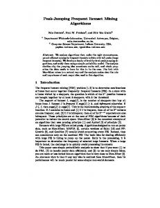
FP-growth uses a combination of the vertical and horizontal database layout to store the database in main memory. Instead of storing the cover for every item in the database, it stores the actual transactions from the database in a trie structure and every item has a linked list going through all transactions that contain that item. This new data structure is denoted by FP-tree (Frequent-Pattern tree) [5]. Essentially, all transactions are stored in a trie data structure. Every node additionally stores a counter, which keeps track of the number of transactions that share the branch through that node. Also a link is stored, pointing to the next occurrence of the respective item in the FP-tree, such that all occurrences of an item in the FP-tree are linked together. Additionally, a header table is stored containing each separate item together with its support and a link to the first occurrence of the item in the FP-tree. In the FP-tree, all items are ordered in support descending order, because in this way, it is hoped that this representation of the database is kept as small as possible since all more frequently occurring items are arranged closer to the root of the FP-tree and thus are more likely to be shared. For example, assume we are given a transaction database and a minimal support threshold of 2. First, the supports of all items is computed, all infrequent items are removed from the database and all transactions are reordered according to the support descending order resulting in the example transaction database in Table 1. The FP-tree for this database is shown in Figure 1. Given such an FP-tree, the supports of all frequent items can be found in the header table. Obviously, the FP-tree is
tid 100 200 300 400 500 Table 1: database.
X {a, b, c, e, f } {a, b, c, d, e} {a, d} {b, d, f } {a, b, c, e, f }
An example preprocessed transaction null
header table a
4
b
4
c
3
d
3
e
3
f
3
a:4
b:3
b:1
d:1
c:3
d:1
f:1
d:1
e:2
e:1
f:2
item support node−link
Figure 1: An example of an FP-tree.
just like the vertical and horizontal database layouts a lossless representation of the complete transaction database for the generation of frequent itemsets. Indeed, every linked list starting from an item in the header table actually represents a compressed form of the cover of that item. On the other hand, every branch starting from the root node represents a compressed form of a set of transactions. Apart from this FP-tree, the FP-growth algorithm is very similar to Eclat, but it uses some additional steps to maintain the FP-tree structure during the recursion steps, while Eclat only needs to maintain the covers of all generated itemsets. The FP-growth algorithm is given in Algorithm 2. Algorithm 2 FP-growth Input: D, σ, I ⊆ I (initially called with I = {}) Output: F [I](D, σ) 1: F[I] := {}; 2: for all i ∈ I occurring in D do 3: Add I ∪ {i} to F[I]; Di := {}; H := {}; 4: 5: for all j ∈ I occurring in D such that j > i do if support(I ∪ {i, j}) ≥ σ then 6: 7: Add j to H; 8: for all transaction X ∈ D with i ∈ X do Add X ∩ H to Di ; 9: 10: Compute F[I ∪ {i}](Di , σ) recursively; Add F[I ∪ {i}] to F [I]; 11: At lines 5–7, all frequent items are computed and stored in the header table for the FP-tree representing Di . This can
be efficiently done by simply following the linked list starting from the entry of i in the header table. Then, at every node in the FP-tree it follows its path up to the root node and increments the support of each item it passes by its count. Then, at lines 8,9, the FP-tree for the i-projected database is built for those transactions in which i occurs, intersected with the set of all j > i, such that {i, j} is frequent. These transactions can be efficiently found by following the nodelinks starting from the entry of item i in the header table and following the path from every such node up to the root of the FP-tree and ignoring all items that are not in H. If this node has count n, then the transaction is added n times. Of course, this is implemented by simply incrementing the counters on the path of this transaction in the new FP-tree by n. However, this technique does require that every node in the FP-tree also stores a link to its parent. The only main advantage FP-growth has over Eclat is that each linked list, starting from an item in the header table representing the cover of that item, is stored in a compressed form. Unfortunately, to accomplish this gain, it needs to maintain a complex data structure and perform a lot of dereferencing, while Eclat only has to perform simple and fast intersections. Also, the intended gain of this compression might be much less than was hoped for. In Eclat, the cover of an item can be implemented using an array of transaction identifiers. On the other hand, in FP-growth, the cover of an item is compressed using the linked list starting from its node-link in the header table, but, every node in this linked list needs to store its label, a counter, a pointer to the next node, a pointer to its branches and a pointer to its parent. Therefore, the size of an FP-tree should be at most 20% of the size of all covers in Eclat in order to profit from this compression. To support these observations, we performed several experiments on a wide variety of different datasets. Due to space limitations, we will only consider 2 of them in this paper. For more results, we refer the interested reader to [4]. Here, we present our results on a synthetic data set generated by the program provided by the Quest research group at IBM Almaden [3], which is a dense dataset that contains 100 000 transactions over 1 000 items. Also, we report our results on the BMS-WebView-1 data set which contains several months worth of click-stream data from an e-commerce web site [6]. This is a sparse dataset containing 59 602 transactions over 498 items. Table 2 shows for these datasets the size of the total length of all arrays in Eclat (||D||), the total number of nodes in FP-growth (|FP-tree|) and the corresponding compression rate of the FP-tree. Additionally, for each entry, we show the size of the data structures in bytes and the corresponding compression of the FP-tree. As was reported in [5], the number of nodes in the FPtree is significantly smaller than the size of the database, but when the actual size of the nodes is taken into account, the FP-tree representation is often much larger than the plain array based representation. Furthermore, the Eclat algorithm performs most of the time significantly better than the FP-growth algorithm. Due to space limitations and since the main focus of this paper is on memory usage, we do not report specifics of these performance experiments. For these results, we refer the interested reader to [4].
Data set T40I10D100K BMS-Webview-1
||D|| 3 912 459 : 15 283K 148 209 : 578K
|FP-tree| 3 514 917 : 68 650K 55 410 : 1 082K
|FP-tree| ||D||
89% : 449% 37% : 187%
Table 2: Memory usage of Eclat versus FP-growth.
3.
MEDIC
If the amount of available main memory is not sufficient to store a complete transaction database, then the efficient depth-first algorithms are generally not able to start. The approach proposed to solve this problem for the FPgrowth algorithm is to create an i-projected database on disk for any item i ∈ I and then mine each projected database separately [5]. Obviously, this approach can be used for any frequent itemset mining algorithm, but unfortunately, it is not feasible for large databases since the cumulated size of all i-projected databases is much larger by orders of magnitude. Note that this strategy also inherently sorts the entire database. However, when the database is lexicographically sorted, using the imposed ordering on the items, a very simple optimization technique can be used to reduce memory usage of the Eclat algorithm, resulting in an even more efficient algorithm, which we call Medic. Let I = {i1 , . . . , in } be all frequent items occurring in D in ascending order of support. Let T [0] denote the smallest item in a given transaction T with respect to the imposed ordering. The Medic algorithm is given in Algorithm 3. For
5–13. Additionally, after generating all these itemsets, the cover of i can be removed from main memory, since it is no longer needed by the algorithm (line 14). After that, the transaction identifier of the current transaction is added to the covers of all items occurring in that transaction. Obviously, this algorithm uses much less memory than Eclat because the database is never entirely loaded into main memory. Indeed, while Eclat initially stores all covers of all items in main memory, Medic only stores the covers of all items up to the currently read transaction and removes them as soon as the item can no longer occur in any forthcoming transaction. By initially reordering all items in ascending order of support, we make sure that this removal of covers happens soon, but we also make sure that the covers of very frequent items only get filled while most other covers have already been deleted. Note that the algorithm in general also performs much better, when sorting the database is not taken into account, since the intersections it needs to perform to count the support of the itemsets are applied to shorter tidlists (or diffsets).
4. Algorithm 3 Medic Input: D, σ Output: F [{}](D, σ) 1: for all i ∈ I do 2: cover ({i}) := {}; 3: F[{}] := {}; 4: for all (tid , T ) ∈ D do 5: for all i ∈ I such that i < T [0] and {i} ∈ / F [{}] do 6: Add {i} to F [{}]; 7: Di := {}; 8: for all j ∈ I such that j > i do 9: C := cover ({i}) ∩ cover ({j}); 10: if |C| ≥ σ then 11: Di := Di ∪ {(j, C)} 12: Compute F [{i}](Di , σ) using the Eclat algorithm; 13: Add F [{i}] to F [{}]; 14: Remove i and cover ({i}) from memory; 15: for all i ∈ T do 16: Add tid to cover ({i}); correctness of the algorithm, we add a transaction to the end of the database containing a new item, denoting the end of the database. In this way, the outer loop is executed one last time. Essentially, the algorithm generates all itemsets containing item i as soon as there can be no transactions anymore that contain i. More specifically, the algorithm processes the transactions one at a time in lexicographical order. For each item i that is ordered before the smallest item in the current transaction, we know it can no longer occur in the database, and hence, we can already generate all frequent itemsets containing i. This is exactly what happens on lines
EXPERIMENTAL EVALUATION
In this section, we compare the memory usage of Medic and Eclat on the same datasets used before. Figure 2 shows the maximal amount of memory used by the two algorithms for varying minimal support thresholds. As can be seen, Medic uses around half of the memory that is used by Eclat for the sparse dataset. Unfortunately, this effect can not be seen for the dense dataset. Indeed, when transactions contain a lot of items, and a lot of items have very high support, the major part of the database will remain in main memory until these items have been processed. Figure 3 shows the memory usage of both algorithms during a single run. These figures clearly explain what happens during the scan of each database. As can be seen, the BMSWebview-1 dataset runs perfectly as is intended by Medic. That is, equal amounts of covers of items are continuously created and removed. On the other hand, it can be seen that the dense dataset almost does not benefit at all. As already explained for the previous experiment, and supported by this experiment, this dataset mostly contain items with very high supports.
5.
CONCLUSIONS
In this paper we focus on the main problem with which current state of the art frequent itemset mining algorithms still have cope with. That is, if databases are too large to fit into main memory, they are simply not able to run. First we presented a rigorous comparison of two well known algorithms that were never compared before, namely Eclat and FP-growth. We pointed out several interesting aspects of both algorithms and have shown that Eclat uses much less memory than FP-growth for most datasets. If the Eclat algorithm still uses too much memory, a new
600
algorithm, Medic, is proposed, which is based on a very simple and elegant technique that essentially uses an optimized version of the Eclat algorithm on a sorted database and already generates all frequent itemsets that can no longer be supported by transactions that still have to be processed. In this way, the algorithm no longer has to maintain the covers of all past itemsets into main memory. The experiments show the effectiveness of the technique for sparse databases. In the case of dense databases, the problem still remains.
Medic Eclat
550
memory (in KB)
500 450 400 350 300 250 200 150 30
40
50
60
70
80
90
100
minimal support
(a) BMS-Webview-1 15500
Medic Eclat
memory (in KB)
15000 14500 14000 13500 13000 500 550 600 650 700 750 800 850 900 950 1000 minimal support
(b) T40I10D100K Figure 2: Memory usage for varying minimal support thresholds.
600
Medic Eclat
memory (in KB)
500 400 300 200 100 0
(a) BMS-Webview-1 16000
Medic Eclat
14000
memory (in KB)
12000 10000 8000 6000 4000 2000 0
(b) T40I10D100K Figure 3: Memory usage during a single run.
Acknowledgements We wish to thank Blue Martini Software for contributing the KDD Cup 2000 data [6].
6.
REFERENCES
[1] R. Agrawal, T. Imielinski, and A.N. Swami. Mining association rules between sets of items in large databases. In Proceedings of the 1993 ACM SIGMOD International Conference on Management of Data, pages 207–216. ACM Press, 1993. [2] R. Agrawal, H. Mannila, R. Srikant, H. Toivonen, and A.I. Verkamo. Fast discovery of association rules. In Advances in Knowledge Discovery and Data Mining, pages 307–328. MIT Press, 1996. [3] R. Agrawal and R. Srikant. Quest Synthetic Data Generator. IBM Almaden Research Center, San Jose, California, http: //www.almaden.ibm.com/cs/quest/syndata.html. [4] B. Goethals. Efficient Frequent Pattern Mining. PhD thesis, transnational University of Limburg, Belgium, 2002. [5] J. Han, J. Pei, Y. Yin, and R. Mao. Mining frequent patterns without candidate generation: A frequent-pattern tree approach. Data Mining and Knowledge Discovery, 2004. To appear. [6] R. Kohavi, C. Brodley, B. Frasca, L. Mason, and Z. Zheng. KDD-Cup 2000 organizers’ report: Peeling the onion. SIGKDD Explorations, 2(2):86–98, 2000. http://www.ecn.purdue.edu/KDDCUP. [7] N. Pasquier, Y. Bastide, R. Taouil, and L. Lakhal. Discovering frequent closed itemsets for association rules. In Proceedings of the 7th International Conference on Database Theory, volume 1540 of Lecture Notes in Computer Science, pages 398–416. Springer, 1999. [8] M.J. Zaki. Scalable algorithms for association mining. IEEE Transactions on Knowledge and Data Engineering, 12(3):372–390, May/June 2000. [9] M.J. Zaki and K. Gouda. Fast vertical mining using diffsets. In Proceedings of the 9th ACM SIGKDD International Conference on Knowledge Discovery and Data Mining. ACM Press, 2003. [10] M.J. Zaki and C.-J. Hsiao. CHARM: An efficient algorithm for closed itemset mining. In Proceedings of the 2nd SIAM International Conference on Data Mining, 2002. [11] Z. Zheng, R. Kohavi, and L. Mason. Real world performance of association rule algorithms. In Proceedings of the 7th ACM SIGKDD International Conference on Knowledge Discovery and Data Mining, pages 401–406. ACM Press, 2001.