Brooklyn College, City University of New York. In previous ... It is now clear that neither humans nor pigeons behave quite as described by SDT in the form.
From M. L. Commons, A. Nevin, & M. C. Davison, (Eds). 1991. Signal Detection: Mechanisms, Models, and Applications. Hillsdale, NJ: Erlbaum (Chapter 6, pages 121-138).
Memory Limitations in Human and Animal Signal Detection Sheila Chase Hunter College, City University of New York Eric G. Heinemann Brooklyn College, City University of New York In previous volumes of this series, we described a general theory of memory and decision making that accounts for phenomena as diverse as probability learning, categorization, concept formation, and pattern recognition (Chase, 1983; Heinemann, 1983a; Heinemann & Chase, 1990). In this chapter we shall discuss how this theory is related to signal detection theory (SDT), and attempt to account for some of the differences between the behavior predicted by SDT and that actually observed. (The problems discussed in this chapter concern “recognition” rather than “detection” but to facilitate communication we shall use the well-known terminology of SDT). We shall limit our discussion here to decisions involving stimuli that induce sensations which vary along a single intensitive dimension, such as loudness or brightness. It is now clear that neither humans nor pigeons behave quite as described by SDT in the form presented by Swets, Tanner, and Birdsall (l96l). For example, the basic measure of sensitivity, d´, is affected by factors not treated by the theory. Four such factors will be considered here: (1) the occurrence of responses that are independent of stimulus value, guessing, (2) improvements in sensitivity that occur during discrimination training (Chase, Bugnacki, Braida, & Durlach, 1983; Heinemann & Avin, 1973; Swets & Sewall, 1963), (3) the dependence of d´ for any particular pair of stimuli upon the range of stimulus values presented during the experiment (Braida & Durlach, 1972; Chase, 1983), (4) the dependence of d´ on the position of the stimulus pair within the range (Braida & Durlach, 1972; Weber, Green, & Luce, 1977). According to our theory, a relatively small amount of information is available at the time a decision is made. As the available information increases, performance approaches that of the optimal statistical decision maker, as specified in SDT. Changes in the information on which decisions are based are reflected in changes in observed sensitivity. Our memory and decision model was originally developed to account for data obtained from experiments in which the stimuli were lights or sounds varying only in intensity and the observers were pigeons (Heinemann & Chase, 1975). In these experiments, two or more stimuli were presented repeatedly in random order for classification, a procedure referred to as the method of single stimuli. The pigeons initiated each stimulus presentation by pecking on a key located in the center of the response panel. After each stimulus presentation, the pigeons were required to peck at one of two or more choice keys which differed in location. Pecks at only one of the choice keys were considered correct on a given trial. In most of our experiments the correct choice was cued by the intensity of white noise or by the luminance of a rectangular translucent screen (display key) located above the row of choice keys. The trial ended when a choice key was pecked. A correct choice was followed by presentation of food; an incorrect choice, shortly thereafter, by another presentation of the same stimulus (correction procedure). Only results obtained on first presentations are considered here. Sessions usually ended when 80 or 100 correct choices had been made.
In the experiments to be reported here the number of stimuli to be classified varied from 2 to 13. In two-choice experiments, the proportion of responses to one of the keys was plotted against stimulus value. From these psychometric functions, or choice curves, d´ may be obtained for pairs of stimuli by treating "hits" as responses to the high-intensity key given the more intense of the two stimuli and "false alarms" as responses to this key given the less-intense stimulus. For experiments involving more than two choices, d´ was obtained using a technique described by Durlach and Braida (1969). In the latter experiments, percent correct and information transmitted were also used as measures of performance. VARIABLES AFFECTING SENSITIVITY TO INTENSITY DIFFERENCES If the stimuli to be categorized are two sounds of slightly different intensities, months of training may be required before there is any evidence that the pigeon is discriminating between the stimuli. Results of an experiment in which the difference between two levels of white noise was varied are shown in Fig. 6.1.
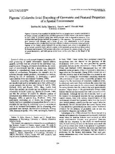
FIG. 6.1 The proportion of R1 responses made in the presence of S1 solid line) and in the presence of S2 broken line). Each panel shows results for a single pigeon trained to discriminate between two levels of white noise differing by the amount shown in the panel (from Heinemann, 1983b).
Fig. 6.1 shows how the proportion of trials on which the pigeon chooses one of the keys changes with training. At first this key is chosen almost equally often in the presence of each of the two sounds. As learning progresses, the curves separate (d´ computed from these sets of "hits" and "false alarms" increases). The number of training trials over which performance remains at chance, called the presolution period (PSP), depends on the intensity difference, as does the asymptotic separation between the two curves. The larger the intensity difference, the shorter the presolution period and the greater the separation. Heinemann (1983b) has shown that this relationship is what one would expect if, during the presolution period, the observer were
acting as a detector of the statistical association between the sensory events induced by the two stimuli and the outcomes of his behavior. As the difference between the average sensory effects induced by the stimuli increases, fewer trials (observations) are required to decide that the stimuli are differentially associated with the outcome of the decision. As a result of a sequential analysis (see Wald, 1947), the observer comes to “attend” to those aspects of the situation (complex of sensations) that are significantly associated with the outcomes of the two choices. When humans serve as psychophysical observers, this presolution period can usually be bypassed simply by telling them which aspects of the situation are relevant. Even with humans, however, substantial training may be required before judgments become stable (Chase et al., 1983; Swets & Sewall, 1963). In order to observe how a discrimination develops, Heinemann and Avin (1973) trained pigeons with a set of 10 sound intensities covering a range of 38 dB. The pigeons were rewarded for pecking on one key in the presence of any of the 5 lowest intensities, and for pecking on the other key in the presence of any of the 5 highest. Fig. 6.2 shows the proportions of responses to the high-intensity key as a function of stimulus intensity. Data are shown for 10-day blocks, with the first function plotted against the actual stimulus values and successive functions each moved to the right by an arbitrary amount. Note that for all birds the curve for the first l0-day block is quite flat. As training progresses, the curves steepen. By the end of training, the proportion of responses to the key that was correct for the higher intensities resembles the psychometric functions obtained by Swets, Tanner, and Birdsall (1961) for human subjects. According to the version of SDT they present, the sensory effects induced on repeated presentations of a stimulus are normally distributed and of equal variance. In Fig. 6.3, seven such hypothetical sensory effect distributions are shown. In the Heinemann and Avin (1973) experiment, the pigeon must decide which of the two key choices, R1, or R2, will be rewarded in the presence of the sensation experienced on a given trial. According to SDT, the proportion of trials on which each response is made in the presence of each stimulus depends on the difference between the sensory effects induced by that stimulus and the criterion, C, where C is a fixed value of sensory effect. R1, is made if the sensory effect produced by the stimulus falls below the criterion; R2 is made if it falls above the criterion. The steepness of the psychometric function, and hence d´, depends on the variance of the sensory effect distributions. The position of the function along the stimulus axis depends on the position of the criterion.
FIG. 6.2 Proportion of R1 responses as a function of stimulus intensity, at various stages of training. Moving from left to right, the curves represent the results obtained on successive blocks of 10 days. The first curve is correctly placed in the coordinate system, the second curve has been moved to the right by 30 dB, and each of the remaining curves has been moved to the right 15 dB more than the immediately preceding one (from Heinemann & Avin, 1973).
FIG. 6.3 Assumed distributions of sensory effects induced by repeated presentations of each of seven different stimuli.
Stimuli corresponding to sensory effect distributions that fall essentially to only one side of the criterion (here distributions 1 and 7) should yield R2 proportions close to 0 and 1.0. As shown in Fig. 6.2, early in training errors occur in the presence of stimuli that are rarely misclassified at the end of training (here the 67 and 99 dB SPL sound intensities). Heinemann and Avin (1973) assumed that such errors are the result of “inattention” to the relevant stimulus dimension, specifically, that on a fraction of the trials the subject’s choice is not based on sound intensity. As can be seen in Fig. 6.1, key choice is independent of sound intensity during the presolution period. The first 10-day block undoubtedly includes choices made during the presolution period. It is therefore not surprising that the choice curve for the first 10-day block is quite flat. Even after the presolution period is over, however, the proportion of trials on which the pigeons
choose the high-intensity key in the presence of each of the end stimuli only gradually approaches 0 and 1.0. It appears that, even after the pigeon learns that sound intensity is relevant, it does not consistently base its choice on this dimension. An experiment of Heinemann, Avin, Sullivan, and Chase (1969) showed that the asymptotes of the choice curves are affected by training conditions. These investigators trained pigeons to choose between two pecking keys on the basis of two levels of white noise intensity. The birds were then tested with 13 sound intensities covering a range from 65 to 100 dB SPL, a procedure referred to in the animal learning literature as a generalization test, since new stimuli are presented (usually without reward) and the probability of occurrence of previously trained behaviors is examined. The test data for birds trained with intensity differences of 29, 7, and 2.3 dB are shown in Fig. 6.4. Here, as in the Heinemann and Avin (1973) experiment, the choice curves resemble the functions one would expect to obtain if the decision process were that described in Fig. 6.3. However, close inspection shows that the high-intensity key is chosen on a substantial number of trials on which one of the lowest intensities was presented. This is especially clear in the result for birds trained on the smallest intensity difference, 83 vs. 85.3 dB (Row 3). The form of the psychometric function may differ even more drastically from the ogival form predicted by SDT when training is done with two closely spaced stimuli, but the stimuli presented during the generalization test that follows training cover a very large range. Under these conditions the generalization curves obtained may be nonmonotonic, that is, choice proportions in the presence of stimuli at the lower and upper end of the continuum may approach 0.5. Curves such as these were obtained by Siegel and Church (1984), who trained rats to discriminate between two signal durations. Nonmonotonic stimulus generalization curves were also obtained by Ernst, Engberg, and Thomas (1971) for light intensities, and by Lawrence (1973) for sound intensities. Monotonic choice curves with asymptotes above 0 and below 1.0 can be fit reasonably well using the SDT model described in Fig. 6.3, provided that the effects of inattention are taken into account. A correction for inattention was used in fitting the smooth curves shown in Figs. 6.2 and 6.4. However, Heinemann and Avin (1973) found that even when measures of sensitivity were corrected for the presumed effects of inattention, sensitivity increased with training. This finding strongly suggests that factors other than improved attention are responsible for some of the increases in d´ with training. The rationale for the correction for inattention and the procedure for applying it are described fully in Heinemann et al. (1969). This correction may be applied to nonmonotonic functions as well (see Heinemann & Chase, 1975). While the correction is of some use as a complement to SDT (see also Blough & Blough, 1989; Church & Gibbon, 1983), it cannot fully extricate SDT from the difficulties that have been discussed. In addition to depending on the amount of training, and the distance of the test stimuli from those used in training, estimates of sensitivity also depend strongly on the context in which the stimuli are presented. Here, context refers to the set of stimuli to which the observer is exposed in an absolute identification task.
FIG. 6.4 Distribution of choices obtained during generalization tests following training to discriminate between levels of white noise differing by 29 dB (top row), 7 dB (middle row) and 2.3 dB (bottom row). Each panel shows results for one pigeon (from Heinemann, Avin, Sullivan, & Chase, 1969).
The important effects of context on measures of sensitivity were highlighted in 1956 by George Miller, who pointed out that humans can identify only about “7 plus or minus 2” unidimensional stimuli with perfect accuracy. Adopting the graphical presentation used by Miller, Fig. 6.5 shows the relationship between information transmitted (number of items correctly identified, expressed as a power of 2) and input information (number of equally probable items in the set to be identified). The data shown were obtained from pigeons, humans, and monkeys trained to identify luminance levels that would rarely be confused if they were presented in pairs (Chase, Murofushi, & Asano, 1985). The pigeons and monkeys were trained to make absolute identifications of three, seven, and nine stimuli. Absolute identification by humans of the nine stimuli used in the monkey experiment is shown for comparison purposes. Both the monkeys and the pigeons were able to identify three luminance levels virtually without error. For three stimuli, information transmitted is 1.6 bits. As the number of stimuli was increased from three to five, information transmitted increased to 1.8 bits for the pigeons and to 2.0 for the monkeys. This value decreased slightly as the number of stimuli was increased to nine. Clearly, information transmitted does not increase indefinitely as the number of stimuli presented for identification increases. The dotted lines in this figure are functions predicted by our model.
FIG. 6.5 Transmitted Information as a function of input information. The theoretical curves differ in sample size. Perfect performance is shown by the diagonal line.
Since most errors in absolute identification involve confusions between adjacent stimuli, it is not surprising that more errors are made as the number of equally spaced stimuli within a fixed range is increased. What is surprising is the finding that, beyond a certain point, increasing the separation between adjacent stimuli does not improve performance. This phenomenon, the range effect, was first observed by Pollack (1952) who found little improvement in absolute identification of tones differing in frequency with a 20-fold increase in stimulus spacing. Braida and Durlach (1972) examined performance of human observers in an absolute identification task involving 10 intensities (equally spaced on a logarithmic scale) of a 1,000-Hz tone. As the range of stimulus intensities was increased from 2.5 to 3.6 log units, performance improved, but a further increase in the range from 3.6 to 5.4 log units had little effect on performance. Pigeons trained on an absolute identification task similar to that of Braida and Durlach, but involving nine light intensities, also failed to improve as the range was increased, in this case from 3.0 to 3.8 log units (Chase, 1983). Not only is d´ for a pair of stimuli affected by the range of the set of stimuli of which they are a part, but also by the position of the stimuli within the range. Stimuli near the ends of the range are identified more accurately than those in the center (Braida & Durlach, 1972; Eriksen & Hake, 1957). Such anchor or edge effects cannot be attributed completely to the fact that confusions involving the end stimuli are one-directional. Weber, Green, and Luce (1977) corrected their data for this factor and still found that the end stimuli were identified with greater accuracy. Within the SDT framework, Berliner, Braida, and Durlach (1977) and Berliner, Durlach, and Braida (1978) separated the effects of bias from those of resolution. Their analysis clearly showed that
sensitivity to the intensity difference between adjacent stimuli, as indexed by d´, depends on the position of the stimulus pair within the range. They suggested that the end stimuli act as anchors, and that the observers measure the distance of the various stimuli from these anchors with a noisy ruler. This notion was formalized by Braida et al. (1984) in their perceptual anchor model of context coding. When describing their performance in an absolute identification task, human subjects often refer to the end stimuli as reference points on which their judgments are based. However, the edge effect is not a phenomenon peculiar to human observers. Monkeys trained to make absolute identifications of light intensities also show greater sensitivity to stimulus differences near the ends of the range (Chase et al., 1985). DESCRIPTION OF THE MODEL Although our model of memory and decision processes was not designed to account for psychometric functions with asymptotes other than 0 or 1.0, or for changes in d´ as a function of variables that should have no effect on the internal representation of the stimuli, it does so quite well. The model, as it applies to decisions involving stimuli varying only in intensity or duration, will be outlined briefly. A number of simplifying assumptions are made in this presentation of the model. A more detailed description of the model and illustrative data can be found in previous volumes of this series (Chase, 1983; Heinemann, 1983a; 1983b; Heinemann & Chase, 1990). Some of the processes and the parameters to be described may seem arbitrary to a reader unfamiliar with these chapters. However, in most cases the processes postulated and parameters suggested are based on extensive empirical work, and on considerations that arise when the model is applied to several situations that are beyond the scope of this chapter, for example, situations that involve multidimensional stimuli, including those that give rise to the phenomena of blocking and overshadowing (Chase & Heinemann, 1972; Heinemann & Chase, 1975), and pattern recognition (Heinemann & Chase, 1990). The model exists in the form of a computer program. Tests of the model are made by comparing simulated with actual behavior. The assumptions are: 1. After the pigeon has learned that input from particular sensory channels is relevant to the outcome of its behavior, information coming from these channels (during any particular trial) is placed into long-term memory (LTM) (see Heinemann 1983a, 1983b). This information is entered on a record which shows the sensation experienced, the response made, and the outcome of the response (e.g., whether or not reward followed). While a record resides in LTM, Gaussian noise is added to the value of the experienced sensation. Prior to the end of the PSP, the memory contains no information regarding the relevant stimuli. It does, however, contain information regarding the response and the outcome, in particular, whether or not the response made was followed by reward. 2. On each trial, a record is placed in a randomly selected location in memory, displacing the record previously in this location. The number of records contained in this memory is limited. The early stages of learning following the PSP thus consist primarily of the replacement of records that lack stimulus information. 3. When a stimulus is presented, a small sample of the records which show that a reward was received is drawn randomly from memory. Our computer simulations and data suggest that the number of records in the sample is between 3 and 15. The response made depends completely on the present sensation, which we shall refer to as the current input, and the information available in this sample of records from LTM. When a sample contains some records with stimulus information as well as some that lack such information, only the former are used. We tentatively
assume that, following the presolution period, samples are drawn until a sample is obtained that includes at least one record that contains stimulus information. Resampling does not go on indefinitely, however. After perhaps 10 unsuccessful attempts to find stimulus information, the choice is made on the basis of response/reward information alone.
FIG. 6.6 A sample of four records retrieved from the LTM. The choice of response is based on the probability densities at the point labeled “current input.” (See text.)
4. The decision process is illustrated in Fig. 6.6. The figure shows four records that provide stimulus information. The Gaussian distributions each represent a previously experienced sensation. The value of the retrieved sensation, for example, the remembered loudness, can be thought of as fluctuating during the decision process, in which case the distributions shown in Fig. 6.6 represent momentary loudness values. In our simulations, the remembered sensation values are specified as points on a decision axis that is scaled in standard units (i.e., standard deviation units). Gaussian noise is added to the values retrieved from LTM (those forming the sample). The degree to which distributions associated with different response labels overlap depends on the separations among the stimuli used in training. However, note that, although three distributions in Fig. 6.6 bear the same response label, R2, indicating that they represent remembered sensations induced by the same stimulus, the means of these distributions are different. That the memories of sensations induced by the same physical stimulus are here represented by distributions that have different means is a consequence of the assumption that remembered sensations stored in LTM are represented by Gaussian distributions, and that each retrieved record represents a sensation selected at random from such a distribution. We assume that the Gaussian noise arises from several sources, among these are variability in the sensory effects produced by the stimuli, and variance added during storage and retrieval. For simplicity, all sources of variance are assumed to be independent and the variances are combined in this illustration and in our simulations. To select a response, the probability density at the current input is obtained for each record and the densities are summed separately for each response. The response made is the one for which the sum of the probability densities is the highest. If this sum is less than some very small threshold value, (δ), then a new sample is drawn. If repeated resampling fails to provide stimulus information (a probability density greater than δ then a “guess” is made, i.e., the choice made is based only on response/reward information.
THEORETICAL ACCOUNT OF FACTORS AFFECTING SENSITIVITY According to our model the form of psychometric functions, as well as values of sensitivity that may be derived from these functions, is affected by the processes described herein. To simplify exposition, the various processes and their effects are described singly, but they often act together to produce particular effects. (1) Effects of inattention to the relevant stimuli on the asymptotes of the choice curves. In a previous section of this chapter, we presented data indicating that, if psychometric functions are determined throughout the course of training, they typically have asymptotes well above 0 and below 1.0 early in training, but with continued training gradually approach functions that have asymptotes of 0 and 1.0. These data are compatible with the assumption, which underlies the correction for inattention, that at any particular stage of training some of the choices made are independent of stimulus value. The account our model gives of this involves the following considerations: Early in training, the LTM is filled primarily with records that were stored during the PSP. These records contain only response/reward information. Thus, samples drawn from LTM shortly after the end of the PSP will contain no stimulus information on many trials, or will contain only a few records with stimulus information. Under these conditions, the functions will be close to horizontal lines. As training progresses, the average number of records that contain stimulus information increases, resulting in the increased separation between the upper and lower asymptotes of the psychometric functions shown in Fig. 6.2. In more detail, choice functions based on response/reward information alone are horizontal lines, as are those obtained if each sample drawn has only a single record that contains stimulus information. With only a single such record in each sample, the response made will be the one associated with this record, regardless of which stimulus is presented for identification. In what follows, it will be convenient to refer to those records in each sample that contain stimulus information as the effective sample. Recall that, provided a sample contains at least one record with stimulus information, the choice of response will be based solely on the effective sample (Assumption 3). The probability that more than one response will be represented in the effective sample increases as the size of that sample increases. Fig. 6.7 shows the results of computer simulations of how the proportions of R2 responses vary with stimulus value when judgments are based on effective samples of several different sizes and there are two possible choices. For a sample size of 1 the function is a horizontal line. For a sample size of 2 the probability of a correct choice is substantially improved; the asymptotes of this curve are near .28 and .72. A sample size of 18 yields asymptotes close to 0 and 1.0.
FIG. 6.7 Results of a simulation showing the effects of sample size on the psychometric function in a situation in which various signal durations are categorized as “long” or “short.” From Heinemann (1984).
We turn next to nonmonotonic functions such as those obtained by Siege1 and Church (1984). The account our model gives of these deviations from the performance predicted by SDT is based on the following considerations: The nonmonotonic functions under discussion occur when the stimuli used in a generalization test include some that differ greatly from those used in training. When the means of all records in a retrieved sample are at least three standard deviations from the current input, then the probability density at the current input is treated as smaller than δ. When this occurs, the subject will resample, and eventually guess if repeated sampling fails to yield stimulus information. (2) Changes in d´ with training. We now consider how our model deals with changes in sensitivity that cannot be attributed to decreases in the proportion of trials on which the subject guesses. Fig. 6.8 shows the effects of increasing the number of effective records available in the sample on estimates of d´. In this simulation, the LTM was filled with records of sensations induced by two stimuli. Simulations for two stimuli separated by one standard unit (dashed curve) and two stimuli separated by two standard units (solid curve) are shown. As sample size increases, the value of d´ estimated from the choice proportions approaches that defined by the normal-normal equal-variance SDT model. For the dashed curve, this is a d´ value of 1.0; for the solid curve, this is a value of 2.0. Our simulations show that, in the two-choice situation, the difference between the values yielded by our model and SDT becomes negligible for sample sizes of 32 or larger. The reason that our model becomes equivalent to the SDT model for large sample sizes is that, for the conditions under consideration here, the numerous distributions associated with the same response may be represented by a single distribution with a mean equal to the mean of the individual means and a variance equal to the mean of the variances. For practical purposes then, the samples retrieved from memory on different trials may be regarded as identical when the number of records in each sample is very large. It was pointed out earlier that the improvement in choice accuracy with training observed by Heinemann and Avin (1973) cannot be attributed completely to decreased guessing. According to our model, the changes in d´ that occur during training to discriminate or identify stimuli result from a gradual increase in the size of the effective sample, that is, the number of retrieved records that carry stimulus information. Early in training there are very few such records in the average sample. As training progresses, records in LTM containing only response information are replaced by records containing stimulus information as well. Thus, training increases the size of the sample on which decisions are based.
FIG. 6.8 Outcome of a simulation showing the effects of sample size on the value of d´ estimated from the data of the theoretical “pigeon.” The assumed difference between the sensory effects induced by the stimuli presented for discrimination was two standard units in one simulation (solid curve) and one standard unit in the other (broken curve).
(3) The range effect and limits on information transmitted. We turn now to a theoretical account of the limit on transmitted information that Miller (1956) referred to as channel capacity. If two stimuli are sufficiently different from each other, few errors of identification will occur. However, as the number of stimuli presented for identification is increased, the same two stimuli are represented, on the average, by fewer records in each sample retrieved from LTM. This circumstance will cause the number of identification errors to increase. For illustrative purposes let us assume that, on each trial of an absolute identification experiment, a sample of eight records is drawn randomly from the LTM. As noted in a previous section, if the sample does not contain at least one informative record, a new sample will be retrieved, and this process may be repeated several times. However, the decision made is determined by the information contained in a single sample. Thus, a response that is not represented on any record in the sample cannot be made. In a two-choice situation there will be, on the average, four records that provide stimulus information for each of the two responses. If four responses are possible then, on the average, each response will be represented by only two records. In a situation in which eight stimuli are to be identified, each response will be represented, on the average, by only a single record. As the number of responses increases, the amount of stimulus information relevant to each response decreases. In addition, it becomes increasingly likely that the correct response will not be represented at all in the sample. In that case, increasing the separation between adjacent stimuli cannot produce any increase in accuracy. Errors will occur as a result of lack of sufficient information regarding all response alternatives. Thus, the limited number of records available when the decision is made seems to be the factor responsible for the range effect as well as the limit on the number of stimuli that can be identified with complete accuracy. The three theoretical curves shown in Fig. 6.5 differ only in the value assumed for the size of the sample, θ: 6 for the pigeons, 10 for the monkeys, 16 for the humans. These values are crude approximations based on simplifying assumptions, primarily the assumptions that increased training or increased stimulus range would not improve performance. (4) The edge effect. We have also attempted to account for the enhanced resolution of stimulus differences near the ends of the stimulus range, the edge effect. Our simulations show that sensitivity would be highest at the ends of the stimulus range if the subject were to base its decisions solely on samples that contain at least one record representing each of the end stimuli and the rewarded responses. The subject could implement such a procedure by resampling on each trial until this condition is met. It is not clear what mechanism could lead to the systematic resampling needed to account for the edge effect. One possibility we are exploring has as its starting point the fact that the stimuli at the end of the range have a privileged position in that they can be confused only with stimuli to one side of the continuum. This asymmetry may result in more resampling when end stimuli are presented for identification. This asymmetry is also responsible for the greater number of correct identifications of the end stimuli. The percentages of correct responses attained in absolute identification tasks are generally highest for the end stimuli. According to our model, this results in better representation of the end stimuli in the sample, and thus greater accuracy in identification. Simulations, however, have shown that without resampling the magnitude of this effect is not great enough to account for the edge effect. While both humans and monkeys trained on a nine-choice absolute identification task show an edge effect, it is not clear whether the same mechanisms are responsible. It is possible that humans’ sampling strategies are less random than those of monkeys or pigeons, as suggested by the anchor model proposed by Braida et al. (1984).
CONCLUSIONS Our model of memory and decision processes originated from an attempt to apply SDT to data obtained from pigeons. As has been shown, the behavior of pigeons and monkeys, as well as of humans, deviates from that of the ideal statistical decision maker described by the most common version of SDT. We propose here that most of the observed deviations follow readily from the assumption that the subjects’ decisions are based on a relatively small amount of information retrieved from LTM. ACKNOWLEDGMENTS The research reported here was supported by NSF Grant Number BNS-79241070, NIMH Grant Numbers MH18246 and MH40712 and PSC-CUNY Grant Nos. 14002 and 11510E and by computing resources provided by the City University of New York, University Computer Center. We thank Neil A. Macmillan and Hiroshi Yamashita for helpful comments on an earlier draft of this chapter. REFERNCES Berliner. J. E., Braida, L. D., & Durlach, N. I. (1977). Intensity perception: VII. Further data on roving-level discrimination and the resolution and bias edge effects. Journal of the Acoustical Society of America, 61, 1577-1585. Berliner, J. E., Durlach. N. I., & Braida, L. D. (1978). Intensity perception: IX. Effect of a fixed standard on resolution in identification. Journal of the Acoustical Society of America, 64, 687-689. Blough, P. M., & Blough, D. S. (1989). Visual effects of opiates in pigeons: II. Contrast sensitivity to sinewave gratings. Psychopharmacology, 97, 85-88. Braida, L. D., & Durlach, N. I. (1972). Intensity perception: II. Resolution in one-interval paradigms. Journal of the Acoustical Society of America, 51, 483-502. Braida, L. D., Durlach, N. I., Lim, J. S., Berliner, J. E., Rabinowitz, W. M., & Purks, S. R. (1984). Intensity perception: XIII. Perceptual anchor model of context coding. Journal of the Acoustical Society of America, 76, 722-731. Chase, S. (1983). Pigeons and the magical number seven. In M. L. Commons, R. J. Herrnstein, & A. R. Wagner (Eds.). Quantitative analyses of behavior: Discrimination processes (vol. 4. pp. 37-57). Cambridge, MA: Ballinger. Chase, S., Bugnacki, P., Braida, L., & Durlach, N. (1983). Intensity perception: XII. Effect of presentation probability on absolute identification. Journal of the Acoustical Society of America, 73, 219-284. Chase, S., & Heinemann, E. G. (1972). Choices based on redundant information: An analysis of two-dimensional stimulus control. Journal of Experimental Psychology, 92, 161-175. Chase, S., Murofushi, K., & Asano, T. (1985). Memory limitations on absolute identification by monkeys and humans. Presented at the annual meeting of the Psychonomic Society, Boston. Church, R., & Gibbon, J. (1983). Temporal generalization. Journal of Experimental Psychology: Animal Behavior Processes. 8, 165-186. Durlach, N. I., & Braida. L. D. (1969). Intensity perception: I. Preliminary theory of intensity resolution. Journal of the Acoustical Society of America, 46, 372-383.
Eriksen, C. W., & Hake, H. W. (1957). Anchor effects in absolute judgments. Journal of Experimental Psychology, 53, 132-138. Ernst, A. J., Engberg. L., & Thomas, D. R. (1971). On the form of stimulus generalization curves for visual intensity. Journal of the Experimental Analysis of Behavior, 16,177-180. Heinemann, E. G. (1983a). A memory model for decision processes in pigeons. In M. L. Commons, R. J. Herrnstein, & A. R. Wagner (Eds.), Quantitative analyses of behavior: Discrimination Processes (vol. 4, pp. 3-19). Cambridge, MA: Ballinger. Heinemann, E. G. (1983b). The presolution period and the detection of statistical assiociations. In M. L. Commons, R. J. Herrnstein, & A. R. Wagner (Eds.), Quantitative analysis of behavior: Discrimination processes (vol. 4. pp. 21-35). Cambridge, MA: Ballinger. Heinemann, E. G. (1984). A model for temporal discrimination and generalization. In J. Gibbon & L. Allan (Eds.), Annals of the New York Academy of Science (Vol. 423): Timing and time Perception (pp. 361-371). New York: New York Academy of Sciences. Heinemann, E. G., & Avin, E. (1973). On the development of stimulus control. Journal of the Experimental Analysis of Behavior, 20, 183-195. Heinemann, E. G., Avin, E., Sullivan, M. A., & Chase, S. (1969). An analysis of stimulus generalization with a psychophysical method. Journal of Experimental Psychology, 80, 215224. Heinemann, E. G., & Chase, S. (1975). Stimulus generalization. In W. K. Estes (Ed.), Handbook of learning and cognitive processes (vol. 2, pp. 305-349). Hillsdale, NJ: Lawrence Erlbaum Associates. Heinemann, E. G., & Chase, S. (1990). A quantitative model for pattern recognition. In M. L. Commons, R. J. Herrnstein, S. Kosslyn, & D. Mumford (Eds.), Quantitative analyses of behavior: Computational and clinical approaches to pattern recognition and concept formation (vol. 9, pp. 109-126). Hillsdale. NJ: Lawrence Erlbaum Associates. Lawrence, C. (1973). Generalization along the dimension of sound intensity in pigeons. Animal Learning and Behavior, 1, 60-64. Miller, G. A. (1956). The magical number seven, plus or minus two: Some limits on our capacity for processing information. Psychological Review, 63, 81-97. Pollack, I. (1952). The information of elementary auditory displays. Journal of the Acoustical Society of America, 24, 745-749. Siegel, S. F., & Church, R. M. (1984). In J. Gibbon & L. Allan (Eds.), Annals of the New York Academy of Science: Timing and time perception (vol. 423, pp. 643-645). New York Academy of Sciences. Swets, J. A., & Sewall, S. T. (1963). Invariance of signal detectability over stages of practice and levels of motivation. Journal of Experimental Psychology, 66, 120-126. Swets, J. A., Tanner, W. P., & Birdsall, T. G. (1977). Decision processes in perception. Psychological Review, 68, 301-340. Wald, A. (1947). Sequential analysis. New York: Dover. Weber, D. L., Green, D. M., & Luce, R. D. (1977). Effects of practice and distribution of auditory signals on absolute identification. Perception and Psychophysics, 22. 223-231.