merge input example plans which can be generated by classi- cal planners. ..... calls findMergePoint, which identifies S1 as a merge point. It then invokes ...
Merging Example Plans into Generalized Plans for Non-deterministic Environments Siddharth Srivastava
Neil Immerman
Shlomo Zilberstein
Deptartment of Computer Science University of Massachusetts Amherst, MA 01003
{siddharth, immerman, shlomo}@cs.umass.edu ABSTRACT We present a new approach for finding generalized contingent plans with loops and branches in situations where there is uncertainty in state properties and object quantities, but lack of probabilistic information about these uncertainties. We use a state abstraction technique from static analysis of programs, which uses 3-valued logic to compactly represent belief states with unbounded numbers of objects. Our approach for finding plans is to incrementally generalize and merge input example plans which can be generated by classical planners. The expressiveness and scope of this approach are demonstrated using experimental results on common benchmark domains.
Categories and Subject Descriptors I.2 [Artificial Intelligence]: Problem Solving, Control Methods, and Search
General Terms Algorithms, Reliability, Verification
Keywords Agent Reasoning: Knowledge Representation, Planning
1.
INTRODUCTION
Automated planning is one of the most fundamental requirements for the effective development and deployment of autonomous agents. The focus of research in AI planning has been on efficiently finding linear sequences of actions that take a specific problem state to a goal state. While this has led to significant performance improvements, research in planning for partially observable situations has not been as successful. Tree structured plan representations used by current contingent planners [5, 2] tend to grow exponentially in size with increasing numbers of objects to be sensed. In this paper we present an approach for extending the scope and scalability of contingent planning. We propose a novel approach for efficiently constructing program-like generalized plans with branches and nested loops for solving Cite as: Merging Example Plans into Generalized Plans for Nondeterministic Environments, S. Srivastava, N. Immerman, S. Zilberstein, Proc. of 9th Int. Conf. on Autonomous Agents and Multiagent Systems (AAMAS 2010), van der Hoek, Kaminka, Lespérance, Luck and Sen (eds.), May, 10–14, 2010, Toronto, Canada, pp. XXX-XXX. c 2010, International Foundation for Autonomous Agents and Copyright Multiagent Systems (www.ifaamas.org). All rights reserved.
classes of situations or problem instances. These problem instances can have different initial state properties (as in the typical formulation), as well as different object quantities, which has not been addressed before. We assume the framework of contingent planning [1], in which probabilistic information about states and action outcomes is not available, so that the agent needs to plan for the worst case. As an example, consider a fire fighting agent with smoke and heat detectors in a building where a room may be on fire. It can use the smoke detector to isolate the floor with the fire, and heat detectors to isolate the room on fire. It’s task is to extinguish the fire, if present. In addition to problems in scalability due to tree structured solutions, state-of-the-art conditional planners would require absolute precision about the number of floors and rooms on each floor in order to solve this problem (few planning frameworks can even express situations with unknown quantities of objects). Suppose further that the agent has successfully executed such searches under test conditions for a few small buildings using reactive control, or even state-of-the-art planners. Unfortunately, even with this information it is not possible to use existing approaches to reliably construct plans for larger buildings. For the fire fighting agent, reliability is an important factor: generalizations are bound to be incomplete and planning time is limited–the agent should be able to quickly determine possible gaps in its generalization, and request assistance if it is at a building that it cannot search. The approach presented in this paper addresses all of these issues. The main contribution of this paper is an algorithm for constructing generalized plans with complex configurations of loops and branches by generalizing and merging linear plans. The input plans can come from observed behavior traces, or could be generated efficiently by classical planners. In the fire-fighting problem for instance, we compute a plan which loops over floors while using the smoke sensors, and then loops over all the rooms of a floor while using the heat sensors (Fig. 4). Although such solutions appear simple, computing them requires reasoning about loops and approaches incomputable problems such as automated algorithm synthesis. This difficulty is borne out by the near absence of approaches addressing such planning problems. We constrain our plan structures to those for which we can efficiently determine preconditions (including those for loop termination and progress towards the goal); however, in this paper we focus on our approach for computing such plans. Contingent planners typically use abstraction to represent the agent’s belief state [1] efficiently. We use a state abstraction and action mechanism which is relatively new in AI,
but is built upon an established body of work in the static analysis of programs (the TVLA system [9]). In addition to representing belief states, we use this abstraction mechanism for recognizing loop invariants and for compactly representing situations where a certain example plan segment will be useful. In prior work [11], we used this abstraction mechanism for the more limited goal of identifying simple loops in a single classical plan without any sensing actions. While a complete description of all aspects of this state abstraction and action mechanism is beyond the scope of a single paper, we provide the relevant details in the next section, which also lays out our formal foundations, including our observation model and plan representation. The following section presents an overview of our approach for computing plans and contains the main algorithms. Sec. 4 presents some of the results obtained with an implementation.
2.
(isGlass(o)
↔
forGlass(c)) ∧ container(c) ∧ ∃b(bin(b) ∧ in(o, b) ∧ robotAt(b))
in
b1
g
b1
obj; isGlass
bin
in
bin
p1
b2
obj; isPaper p2
b3
in
p1
obj; isPaper in
p2
obj; isPaper
bin
S1
g
obj; isGlass
bin
obj; isPaper
S2
b
in
x
isGlass
obj
bin
isPaper Sa
Figure 1: Abstraction for representing belief states in0 (u, v) := (in(u, v) ∧ u 6= o) ∨ (¬in(u, v) ∧ u = o ∧ v = c) empty 0 (u) := empty(u) ∨ in(o, u) collected0 (u) := collected(u) ∨ o = u
FORMAL MODEL
Running Example In the rest of this paper, we will use the recycling problem as a running example: a recycling robot must pick up objects from a set of bins, perform a sensing action to determine recyclability of the drawn object, and store it in an appropriate container. We represent states of a domain as traditional (two-valued) logical structures over a domain-specific vocabulary of predicates. A state thus consists of a universe of objects, and for every predicate, a set of object-tuples satisfying it. Domains may include first-order integrity constraints that must be satisfied in all instances of the domain. We use the terms “state” and “structure” interchangeably. Each action is specified as a first-order formula defining its precondition, and a set of update formulas defining the new value of each predicate. The following equation shows − the update formula for predicate pi where ∆+ i (∆i ) specifies when pi (¯ x) will be changed to true (false) by the action: p0i (¯ x) := (¬pi (¯ x) ∧ ∆+ ∨ (pi (¯ x) ∧ ¬∆− (1) i ) i ) This first order representation of planning is very standard from a logical point of view and can be easily translated to frame axioms for actions and to successor state axioms in the situation calculus. However, instead of using theorem proving to derive the effects of an action, we use the much more efficient method of formula evaluation on structures. Example The recycling problem can be modeled using the following vocabulary: V = {bin1 , visited1 , object1 , collected1 , empty1 , container1 , forPaper1 , forGlass1 , in2 , isPaper1 , isGlass1 , robotAt1 }. An example structure, S, can be described as follows: the universe, |S| = {b, o, c1 , c2 }, binS = {b}, objectS = {o}, containerS = {c1 , c2 }, forPaperS = {c1 }, forGlassS = {c2 }, inS = {(o, b)}, isPaperS = {o}, robotAtS = {b}, visitedS = {b}. We omit the predicates not satisfied by any tuples. Integrity constraints for the recycling domain would include among others the formulas ∀uvw(in(u, v) ∧ in(u, w) → (v = w ∧ (bin(v) ∨ container(v)))) meaning that each object can be in at most one bin or container, and ∀u(object(u) → (isGlass(u) ↔ ¬isPaper(u))) meaning that objects are either of type paper or of type glass. To keep the presentation simple, we assume here that no bin contains more than one object. The goal condition is that all bins are empty: ∀x(bin(x) → empty(x)). The precondition and updates for the action collect(o, c) are:
in
b2
bin
2.1
Abstract States and Actions
We represent belief states as in prior work [11] which in turn is based on the abstraction methodology of TVLA (Three Valued Logic Analyzer), a system for the static analysis of programs [9]. In this approach, potentially infinite sets of similar concrete structures can be represented using an (abstract) 3-valued structure, where the truth value of a tuple being in a relation may be 1 (present), 0 (not present), or 21 (perhaps present). The universe of such an abstract structure may include summary elements, each of which denotes an arbitrary non-zero number of objects. We draw summary elements using double circles; relations with truth value 12 are drawn using dotted edges, those with truth value 1 are drawn using solid edges and those with truth value 0 are not drawn. For example, in Fig. 1 the abstract structure Sa contains two summary elements, b, x. Intuitively, Sa represents (or “embeds”)1 any concrete structure that contains one or more non-empty bins, (since empty is not written it is false), and one or more objects of unknown type (paper or glass). Since concrete structures must satisfy the integrity constraints, we know that each bin contains exactly one object and no object is in more than one bin. Two structures represented by Sa are drawn at the top of Fig. 1. The set of all concrete states represented by Sa is denoted γ(Sa ). Recall that all states of a domain are required to satisfy the integrity constraints, I. Thus, γ(Sa ) = {S | Sa w S; S concrete; S |= I}. Given a domain, we choose a set, A, of unary predicates to be the abstraction predicates. (The set of observable unary predicates in our examples constitutes the abstraction predicates.) We define the role of an element of a structure to be the set of abstraction predicates it satisfies. In Fig. 1, the role of pi ’s, g and x is {obj}. The canonical abstraction of a concrete structure S # , is the least general abstract structure S that represents S # and has definite truth values for each abstraction predicate [9]. This is computed simply by collapsing all elements of each 1 Formally we say that structure S represents structure T (equivalently, T is embeddable in S), S w T , iff there is an onto function f from the universe of T onto the universe of S such that for any relation symbol Rk , and any elements, t1 , . . . , tk of T , the truth value of R(f (t1 ), . . . , f (tk )) in S, generalizes the truth value of R(t1 , . . . , tk ) in T ( 12 generalizes anything whereas 0 and 1 only generalize themselves).
chosen
isGlass b
in
chosen b
x
in
x
obj
bin
obj
bin
isGlass
Coerce
isPaper
isPaper S1
chosen
isGlass b
in
b
isPaper S0
isGlass
in
bin
obj
bin
b1
b1
chosen Focus(chosen(x))
x
S4
in
Coerce
x
bin
isPaper
S2
in
in
isGlass x
obj
isPaper S5
isGlass b
in
bin b
obj
bin
chosen
Coerce
x
obj
bin
isPaper S3
Figure 2: Focus and coerce. role to one element of that role. The collapsed element is a summary element if there were multiple elements with that role in S # . Truth values of tuples involving summary elements in S are the most specific generalizations of the truth values of tuples they represent in S # . (In Fig. 1 Sa is the canonical abstraction of S1 , and of S2 .) Note that even though they typically represent infinite collections of concrete states, each canonical abstract structure contains at most 2a elements where a is the number of abstraction predicates. Abstract structures thus present an efficient way to model belief states with uncertainty in object quantities.
2.1.1
Action Application on Abstract Belief States
Since we represent belief states using three-valued structures, we can safely apply the (first-order) definitions of the action operators directly to the current belief state to derive the new belief state after the action has been applied. For action, a, and abstract or concrete structure, T , let τa (T ) denote the result of applying action a to T . Fact 1 If S represents S # then τa (S) represents τa (S # ) [9]. Fact 1 should give the reader an idea of the power and generality of the TVLA abstraction methodology. However, to make this useful, we have to make sure that the belief states stay as precise as possible as we repeatedly apply actions, i.e., we want to maintain definite truth values (0,1) whenever possible. While the abstraction is convenient for succinctly representing a large set of possible concrete structures, the designers of TVLA have observed that before an action is applied, it is useful to view some predicates in more detail. They thus introduced the focus operation: given an abstract structure, S, and a formula, φ, with at most one free variable, focus(S, φ) produces a set of structures S1 , . . . , Sk that represent the same set of concrete structures as S, i.e., γ(S) = γ(S1 ) ∪ · · · ∪ γ(Sk ), but such that the truth value of φ is definite in Si , i = 1, . . . k. Given an action a, we automatically generate a set of relevant focus formulas, φ1 , . . . , φt from the ∆± formulas of the action update (Eq. 1), and focus with respect to all of these. We then apply τa to the relevant structures, thus preserving precision. We use the TVLA function coerce to refine or remove any structures that do not satisfy the integrity constraints. Finally, we canonically abstract the result structures to return to the standard, abstract representation, no longer focusing on φ1 , . . . , φt . In Fig. 2, a simple example of focus is shown, where we are focusing on the formula chosen(x) whose meaning might
be that x is the unique argument on which action a will be applied. On the left, structure S1 is shown where chosen has truth value 21 for the element b of role {bin}. When we focus on chosen the result is the three structures on the right representing the situations where chosen has definite truth values and holds for all, some, and none of the elements represented by the summary element b, respectively. On the extreme right, in the presence of the integrity constraint saying that chosen must hold for a unique element of the universe, coerce removes S3 and refines S1 and S2 . This shows how we use focus and coerce to draw-out a representative element from summary elements. Continuing with Fig. 2, as we would expect, the result of drawing-out a representative element from a summary element of a role ({bin}) results in two cases (at the extreme right): one where the drawn out element is the only element of that role, and one where there are more elements of that role. This drawingout mechanism is used to select a unique action argument prior to action application. In the sequel, we will see that the role of an action’s argument ({bin}, to which chosen was set to have the truth value 12 ) gets specified by the corresponding action instance in an example plan. We refer the interested reader to existing literature on TVLA (such as [9]) for further details on focus and coerce.
2.2
Observation Model and Sensing Actions
Contingent plans deal with uncertainty about predicates in the agent’s belief state using observation or sensing actions [1, 5]. We model sensing actions as focus operations w.r.t the respective formulas being sensed. When applied to an abstract state, they return a set of more precise belief states corresponding to the different possible definite truth values of the formula being sensed. For instance, the recycling domain has only one sensing action applicable to a chosen bin marked with the new (not in the domain’s vocabulary) abstraction predicate chosen: senseType(), with the focus formula ∃x(chosen(x) ∧ in(o, x) ∧ isP aper(o)). When applied to an abstract structure (such as S4 or S5 in Fig. 2), it returns structures with different possible types of a single object in the chosen bin. Note that the integrity constraint that each object has a unique type makes either of the predicates isPaper, isGlass sufficient for sensing an object’s type. In addition to uncertainty about predicates, the agent does not have precise information about object quantities. We only require that it has sufficient knowledge to determine whether there are zero, exactly one, or more than one objects of each role at any step.
1 2 3 4 5 6 7 8 9
10 11 12
Input: Existing plan Π, π = (a1 , . . . , an ), S0# Output: Extended version of Π bpπ , bpt ← 0 t← generalize(π, S0# ) mpΠ , mpt ← findMergePoint(Π, t, bpΠ , bpt ) repeat if mpΠ found then bpΠ , bpt ← findBranchPoint(Π, t, mpΠ , mpt ) end if bpΠ found then mpΠ , mpt ← findMergePoint(Π, t, bpΠ , bpt ) addEdges(Π, t, bpt , mpt , mpΠ , bpΠ ) end until new bpΠ or mpΠ not found if bpπ found and mpπ not found then /* A terminal segment of t was not merged */ remainderT ← path added to Π after bpΠ /* Try to create loops in remainderT */ formLoops(remainderT) end return Π Algorithm 1: Branch and Merge
The planning problem Given a set of domain-specific actions, integrity constraints, a goal formula, and an initial belief state Sinit , our objective is to find a generalized plan solving the initial belief state Sinit .
2.3
Plan Representation and Execution
Our representation of generalized plans is similar to that of finite state controllers: a generalized plan is a directed graph whose nodes are labeled with actions and edges are labeled with structures. Edge labels may also include conditions (with the default condition True) under which they may be taken. Execution begins at one of the pre-defined start nodes of the plan. At any stage during plan execution a program-counter (initialized with the start node) labels the active node. The neighbors of a node represent the next possible actions. At each step in plan execution the action labelling the active node is executed; subsequently, an edge satisfied by the current belief state is taken and the neighboring node along this edge becomes the new active node. At any stage, if the next action cannot be carried out, or if a valid edge embedding the resulting belief state cannot be found, the plan execution ends. A generalized plan solves a concrete state S # if every allowed execution of the plansteps on S # starting at an allowed start node ends at a state satisfying the goal; the plan solves a belief state S if it solves every S # ∈ γ(S) from which the goal is reachable. This representation follows standard conventions for control flows. However, for ease in describing the merge operations used during the construction of generalized plans, in Sec. 3 we will work with the dual of this plan representation, where structures label nodes and actions label edges.
3.
MERGING EXAMPLE PLANS
The most significant challenge faced by approaches combining multiple example plans is to determine positions in an existing plan where segments of a new example plan would be useful. This becomes more difficult when the existing plan contains loops. BranchAndMerge (Alg. 1) is a
Input: Sinit , the initial belief state Output: Plan Π Π ← ∅; looseEnds ← Sinit while looseEnds 6= ∅ do Remove S0 ∈ looseEnds S0# ← concrete instance of S0 π0 ← invokeClassicalPlanner(S0# ) Merge(Π, π0 , S0# ) looseEnds ← getLooseEnds(Π) end return Π Algorithm 2: Generalizing and merging examples
greedy algorithm for addressing this problem. It uses abstract structures in plan traces as a compact representation of the infinitely many situations where the subsequent sequence of actions would be useful. The input to Alg. 1 is the existing plan (initially ∅), a new linear example plan and a concrete structure solved by the example plan. Such example plans can be provided from prior experience. Given an abstract structure S0 representing the initial belief state, they can be also generated by existing classical planners as follows: (a) create a concrete member state S0# ∈ γ(S0 ) with specific truth values for the unobservable predicates. The number of universe elements in S0# corresponding to a summary element in S0 can vary; in this paper we used a heuristic process to add at least six elements in S0# for every summary element in S0 . (b) make the appropriate sensing actions for the unobservable predicates as prerequisites for actions which use those predicates (c) solve this problem instance using a classical planner like FF [6]. In the recycling problem, the input to a classical planner can be a problem instance with multiple non-empty bins where each object’s type is “paper”. The collect action’s formulation will require a predicate “sensed” to hold for the object being collected. The sensed predicate on the other hand will only be set by a “senseType” action with no other effect. This problem’s solution plan will use “senseType” actions, but will only solve the problem for “paper” objects. BranchAndMerge proceeds as follows. The example plan is first generalized (line 2). The input to the generalize subroutine is a pair (π, S0# ), where π = (a1 , . . . , an ) is a solution plan for the concrete structure S0# . Plan π is generalized by replacing the action ai ’s arguments by their roles in the # # concrete structure Si−1 (Si# = ai (Si−1 ), i = 1, . . . , n) and including the automatically generated (Sec. 2.1.1) focus formulas. This results in a modified linear plan applicable in the abstract state space, say π 0 . The sequence of intermediate concrete states is then generalized by applying π 0 on the canonical abstraction S0 of S0# , and keeping only those results Si = a0i (Si−1 ) which are consistent with the Si# . This results in an interleaved sequence of structures and actions because only one of the results of the focus operation can be consistent with a concrete state. Structures which are not consistent with the result seen in π at the same step represent possible situations that were not handled by π. These abstract structures can be indexed and stored in a list of “looseEnds” if suggestions for further examples are needed or in a hybrid implementation (Alg. 2). The generalization process is similar to “tracing” [11]. Given an example trace t and an existing plan Π, Alg. 1 uses findMergePoint (lines 3 & 7) to find the index of the
earliest structure in t that is embeddable in a structure in Π. If successful, findMergePoint returns mpΠ and mpt , the node in Π and the index in t corresponding to these structures. A successful search indicates that the new example encountered an instance of a belief state present in Π. However, the subsequent actions in t may not be different from those following mpΠ in Π, or may not handle any new problem instances in addition to those already handled by Π. In order to minimize the new edges added to Π, after finding the merge points, Alg. 1 conducts a search for a branch point using the procedure findBranchPoint. findBranchPoint simultaneously traverses the actions of t and Π starting from the last known merge points mpt and mpΠ , and returns the last node and index where the example trace matched the plan Π. More precisely, starting at the previous merge points mpt , mpΠ it matches successive elements of t with action edges and structure nodes in Π until it finds a node bpΠ in Π and an index bpt for a structure in t such that either (a) none of the successor actions of bpΠ in Π match any of the successor actions of bpt in t, or (b) there is a matching successor action in Π, but its resulting structure does not embed the resulting structure in t. A branch point will not be found only if the example trace after the last merge point is completely subsumed by a path in Π. In this way findBranchPoint gives us a situation where the example trace behaved differently from the existing plan. In general, the search for subsequent merge points can range over all nodes in Π. Allowing merges with any node in Π introduces loops of increasing complexity, which makes it difficult to determine vital properties such as the guaranteed termination of the resulting plan. From this point of view, we limit the set of allowed merge points to non-ancestors of the last branch point and nodes within the same loop. The list of non-ancestors is obtained by running BFS on Π with its edges inverted, and taking the complement of the obtained set of reachable nodes. The resulting plans can be analyzed for preconditions very efficiently. A description of the methods for doing so is beyond the scope of the current paper, but this issue is addressed briefly in Sec. 3.2. The overall BranchAndMerge algorithm works by adding nodes for structures and edges labeled with actions from the branch point to the merge point (bpt , mpt respectively) in the trace t, starting at bpΠ in Π and ending at mpΠ . If the merge point in Π coincides with the previous branch point, Alg. 1 introduces a new loop. If a merge point is not found, all the actions and structures from bpt are added to Π, in a linear path starting at bpΠ . Alg. 1 then calls the formLoops algorithm described in prior work [11] in order to find loops in the path of actions that was added after bpΠ . Given a generalized plan Π with ΠE edges and a new trace t with tn nodes, Alg. 1 runs in time O(ΠE · tn ) and satisfies the following property: Observation 1 In any plan produced by Alg. 1, the shortest path to the goal from any concrete member of the initial belief state is smaller than or equal to the best provided example that solved it. This is because action sequences from example traces are either merged with existing edges that subsume them, or are added to the existing plan. A Hybrid Approach Alg. 1 can be implemented as a part of a proactive algorithm for incrementally generating example plans and merging them (Alg. 2). Alg. 2 uses the list of looseEnds which can be created by the generalize subroutine. It requires a book-keeping subroutine for removing
structures which have been solved from the list looseEnds when example traces are merged with the existing plan Π. A complete implementation of Alg. 2 is left for future work. Quality of Generalization We measure the quality of plans on the basis of the fraction of solvable problem instances that they solve. More specifically, we define Dπ (n) = |Sπ (n)|/|T (n)| where T (n) is the set of solvable problem instances of size at most n, and Sπ (n) is the subset of those that π solves. For example the recycling problem of size n must have n/2 each of bins and bin-contents, yielding a total of 2n/2 instances with different bin contents.
3.1
A Detailed Example
Fig. 3(a) shows a plan segment that collects one object of type paper, moves to the next bin and finds a glass object. S0# is a concrete structure in which more than 2 objects each of type paper and glass have been collected, and two bins remain to be visited. Two of the actions in this example, gotoNextBin and senseType, can have multiple abstract results due to the focus operations described earlier. When applied on an abstract structure with an unknown number of unvisited bins, the two results of the gotoNextBin action correspond to whether or not the next bin is the last unvisited bin, as per the drawing-out operation described earlier (Fig. 2). The senseType action uses the focus operation to enumerate the different possibilities for the type of the object being sensed. Dotted edges in Fig. 3 represent results of these actions that did not occur in the execution of the given example plan on S0# . Fig. 3(b) shows the result of generalizing Fig. 3(a). S0# ’s canonical abstraction, S0 , is identical to S4 , the abstract result of collecting another object of type paper. This is recognized by formLoops (Alg. 1, line 10) because at this stage, the plan Π is empty. formLoops creates a loop by attaching the “collectPaper()” edge to S0 (Fig. 3(c)). The following action edge (gotoNextBin()) from S4# however, is not merged with the edge between S0 and S1 because S5# and its abstraction S5 do not have any elements with the role of “unvisited bins”, thus differing from S1 . Fig. 3(d) shows an example plan for handling a structure identical to S1# , but with the type of the object in the bin set to glass. This plan is also traced in the abstract state space and Alg. 1 is called with the resulting trace and the current generalized plan (shown in Fig. 3(c)). Alg. 1 in turn calls findMergePoint, which identifies S1 as a merge point. It then invokes findBranchPoint, which also returns S1 . This is because the result of the senseType action on S1 is S7 in the generalized trace, where the chosen bin has an object of type glass (unlike S2 , where it was paper). After finding this branch point, Alg. 1 calls findMergePoint again, and this time, cannot find any merge points in the example trace before S11 , which it determines can be embedded in S1 . It returns S1 in Π and S11 in t as the merge point, following which the subroutine addEdges is used to add the structures and actions between S7 and S11 to Π.
3.2
Loop Preconditions
Because this approach stores the abstract structures possible after any action in the computed generalized plans, this information can be used to efficiently find the preconditions or the set of problems that a computed generalized plan solves. These conditions take the form of linear inequalities between the numbers of elements of different roles (the
(a) Example plan execution: #
S0
goToNextBin()
#
S1
#
senseType()
S2
preProc−Paper()
#
S3
collectPaper()
S4
#
gotoNextBin()
S0
gotoNextBin()
#
S5
S6
senseType()
(b) After Tracing: S5 S0
goToNextBin()
S7 S1
senseType()
S1 S2
preProc−Paper()
S3
collectPaper()
(c) After Finding Loops: #
goToNextBin()
goToNextBin()
S1 S5
senseType()
S7 senseType()
S2
S6
(d) Example plan for unhandled structure:
collectPaper()
S0
S8 senseType()
S5
preProc−Paper()
S1
senseType()
#
S7
preProc−Glass()
#
S9
collectGlass()
#
S 10
goToNextBin()
#
S 11
S3
S6
S8
(e) After Generalization and Merge: collectPaper()
S6
senseType()
S5
goToNextBin()
S0
goToNextBin()
S1
S8
senseType() senseType()
S2 S7
preProc−Paper() preProc−Glass()
S3 S9
collectGlass()
S 10
S 12
goToNextBin()
Figure 3: A detailed example for Merge. Dotted edges represent results that did not occur in the example. “role-counts”) and variables representing the number of iterations of each loop. While a description of these methods is beyond the scope of this paper, we quote the results below and refer the interested reader to [12] for details and proofs. We define a simple loop as a cycle of nodes, and a complex loop as a strongly connected component that is not a simple loop. A shortcut in a simple loop is a linear sequence of actions (no branches) starting with a branch caused due to a sensing action in the loop and ending at any subsequent node in the loop that is not after a chosen start node. The start node can be any node, but is common to all of a loop’s shortcuts. Simple loops with shortcuts capture a broad class of nested loops. Extended-LL domains [11] are a class of domains where the unary predicates of a state are sufficient to determine truth values of predicates of higher arities involving the drawn-out objects in that state. Lemma 1. Suppose a simple loop with shortcuts in an extended-LL domain with sensing actions is entered with the role-counts r¯0 at loop node Si . Then sufficient conditions under which the execution of the loop will end via an action branch from a loop node St in the loop, with the role-counts r¯t can be computed in time O(s · ne · m), where m is the number of shortcuts, ne is the number of edges in the simple loop with shortcuts, and s is the maximum number of roles in any structure in the loop. Theorem 1. Let Π be a plan whose loops are simple loops with shortcuts in an extended-LL domain with sensing actions. Sufficient conditions determining the achievable rolecounts for any structure in Π can be computed in time linear in the number of actions in the plan.
4.
IMPLEMENTATION AND RESULTS
We present the results of some of our experiments with an implementation of BranchAndMerge. The test problems were motivated by benchmarks from the international plan-
ning competitions and require solutions with different combinations of loops and branches. Incremental results for each problem are shown in Fig. 4, with segments added due to different examples labeled and drawn with different edge types. The actual outputs are more detailed, and include one iteration of the loop learned using the first example prior to the topmost action shown in the figures. Since the loops tend to get too complex to understand visually, we present modified outputs in order to aid readability: structure-nodes and edge labels for results of sensing actions are not drawn and some action operands are summarized into action names. We present a summary of these results with their incremental domain coverages, and provide representative detailed results and execution times for the recycling problem. The fact that all the loops make progress and terminate can be determined automatically (Lemma 1). Fire Fighting This problem was discussed in the introduction. Smoke can be detected from anywhere on a floor iff one of its rooms is on fire. The agent has smoke and heat sensors; it can use the senseSmoke and goToNextFloor actions to reach the correct floor, and the senseHeat and goToRm actions to find the room on fire. The extinguishFire action can be used to extinguish a fire. The number of rooms and floors in the building are unknown, and unbounded. The first example plan solved an instance of the problem with 6 floors, with 1 room on each floor. None of the floors were smoky in this problem instance (we did this to stress BranchAndMerge; a problem instance with a smoky floor would have extracted more of the solution plan from the first example itself.). The example plan used goToNextFloor to traverse all the floors but found none to be smoky. Since this was the first example, BranchAndMerge called formLoops which created the loop labeled (1) (Fig. 4(a)). The second example plan solved a smaller problem instance. In its initial state, the agent is on the fourth floor of a building with 6 floors and this floor is smoky, but the smoke has not been detected The fire is in room 4; there are 5 rooms on this floor (the agent starts at the fourth floor to
goToNextBin()
senseSmoke−CurFloor() 1
1
2
move(T2, L)
go−UnvisitedRoom−CurFloor()
goToNextFloor()
senseType() 2
senseHeat−CurRoom()
2
forkLift(server, T1)
apply−PaperPreProc(obj)
senseSmoke−CurFloor()
move(T1, L)
collect−Glass(obj) collect−Paper(obj)
4
move(T2, D2)
load(server, T1)
apply−GlassPreProc(obj)
3
1
move(T1,D1)
unload(T1)
go−UnvisitedRoom−CurFloor()
move(T2,L) 3
3
move(T2, D1) forkLift(server, T2)
senseType()
load(server, T2)
4
extinguishFire−CurRoom()
apply−GlassPreProc(obj) collect−Glass(obj)
(a) Fire Fighting
load(server,T2) 4
senseHeat−CurRoom()
go−UnvisitedRoom−CurFloor()
load(monitor, T2)
goToNextBin()
2
apply−PaperPreProc(obj)
move(T2,L) forkLift(server, T2)
move(T2, D3)
unload(T2)
collect−Paper(obj) (b) Recycling
(c) Transport
Figure 4: Segments of computed plans. Circled numbers and edge types label components from different examples.
1 D(n>=8) = 1 0.8
Coverage (D)
make it harder to identify the context – starting at the first floor would have provided a large prefix of actions matching those of Π). The example plan used senseHeat and goToRm actions to visit rooms 1,2, and 3 before reaching room 4, sensing heat, and extinguishing the fire. BranchAndMerge found that the initial structure of this plan was embeddable in the abstract structure in loop 1 (Fig. 4(a)(1)), corresponding to the agent being at any floor of the building. The first senseSmoke action was also merged with (1), but its result and the remainder of the example trace was not embeddable anywhere in the existing plan (Fig. 4(a)(1)). A loop was also detected in the remainder of this trace (Fig. 4(a)(2)). The generalized plan formed using examples (1) and (2) does not solve some boundary cases, for instance when the first floor is smoky or when the first room in a floor has fire. Example plans 3 and 4 handled these situations. However, only two edges were added from these plans, connecting structures already in the generalized plan. In the final plan, there are no unresolved action branches indicating that the goal structure with the fire extinguished is always reached. Recycling This problem was used as the running example and its solution was described in Sec. 3.1. BranchAndMerge creates a loop in this example, illustrating how small examples can be used to identify powerful loops. Example 3 dealt with an unhandled branch caused due to the drawing out of elements from a summary element (last bin was reached), and example 4 handled the case where the last object was of type glass. Transport We have a Y-shaped transport map with depots D1 , D2 , D3 on the end points. Two trucks, T1 and T2 with capacities one and two are originally at D1 and D2 , respectively. The problem is to deliver an unknown number of server crates (from D1 ) and monitor crates (from D2 ) in pairs with one of each kind to D3 . Location L at the center of the Y can be used to transfer cargo between the two trucks. There are two non-deterministic factors in this problem: server crates may be heavy, in which case the simple load action drops them and a forkLift action must be used; crates left at L may get lost if no truck is present. The first example plan delivered 6 pairs of crates to D3 without experiencing heavy crates or losses. The second example found a heavy crate, and delivered it using forkLift actions instead of load; in the third plan a crate left at L was found missing when T2 reached L, and another crate had to be picked up from D1 . The plan computed using these three
0.6
CFF-soln7 Gen(Eg 1) Gen(Eg 1+2) Gen(Eg 1..3) Gen(Eg 1..4)
D(n>=8) = 0.5
0.4 D(n>=8) = 0.25 0.2
0 0
5
10
15 20 Max Number of Bins (n)
25
30
35
Figure 5: Domain coverage of recycling problem plans. Plan Time(s)
Gen(1) 110
Gen(1..2) 129
Gen(1..3) 134
Gen(1..4) 144
CFF-soln7 262
Table 1: Solution Times examples does not handle one case of a server crate being heavy (Fig. 4). This was was handled by example plan 4. Key Observations All the presented solutions solve problems of unbounded sizes. BranchAndMerge adds only necessary segments from example plans. For instance, only edges for the two forkLift actions from the entire second example in transport were added. In fire fighting, the result of senseHeat action in example 4 of the fire fighting problem was directly merged to a structure that had already been handled. Merging plan segments within loops is a powerful technique for increasing the scope of the plan far beyond the individual examples: in recycling, the plan learned using the first example solves only n of the 2n+1 − 1 possible problem instances of size at most n. The second plan covers a single specific problem instance. The generalized, merged result using these two plans solves 2n−1 instances (it assumes that the last two bins have paper). Further Details and Comparison We illustrate the incremental increases in domain coverage discussed above with plots (Fig. 5) and the times (Table 1) taken to generalize and merge input example plans for the recycling problem. Fig. 5 shows that the domain coverage Dπ (n) increases
significantly with each new example plan, and approaches 1 with four examples. Since no other approach can solve these problems due to uncertainties in object quantities, direct comparisons are not feasible. However, to put this in perspective, we compare these results with the domain coverage and execution time for the largest recycling problem instance (with 7 bins) that we could solve using contingentFF [5], a state-of-the-art contingent planner. Given the four example plans for recycling described above, the generalization and merging process produces a near complete solution while taking 45% lesser time than the time taken by contingent-FF to find a plan (CFF-soln7) for 7 bins. Generalized plans for all the other problems discussed above were generated in under 300 seconds and showed similar comparative performance with contingent-FF. Tests were conducted on a 2.5GHz AMD Dual-Core machine with 2GB of RAM.
more exhaustive search and return the merge point which allows the longest segment of the trace to be merged. We also limited the capabilities of BranchAndMerge in this paper to only create loops which can be efficiently analyzed to determine termination and applicability, although a discussion of these methods is beyond the scope of this paper. While there are many directions for future work with ample opportunities for improving these fundamental algorithms, the results already demonstrate applicability and expressiveness not provided by any other existing approach.
7.
Support for this work was provided in part by the National Science Foundation under grants CCF-0541018, CCF0830174 and IIS-0915071.
8.
5.
RELATED WORK
Using loops in plans has been previously proposed and analyzed. Winner and Veloso [13, 14] present methods for converting example plans into plans with branches and loops. However, this approach does not address issues such as determining termination and progress in loops, creation of nested loops and the merging of multiple examples while creating loops. Levesque [8] presents an approach (Kplanner) for finding plans with loops which generalize only a single, user-provided numeric planning parameter. Cimatti et al. [3] consider domains where loops are needed for actions which may have to be repeated for success. Loops created using this approach need not make definite progress, and the resulting plans may execute an unbounded number of operations before achieving the goal. In contrast, our objective is to find loops that make measurable changes and lead to the goal after a finite, computable number of steps. The current authors’ prior work [11] had a similar objective, but only dealt with the more limited problem of recognizing simple loops in a classical plan. Hansen and Zilberstein [4] also present a method for computing policies with loops of actions, but in a setting where probabilities of action outcomes and their rewards are used to determine the action which would lead to the best possible value. Recent approaches for agent programming languages and architectures [7, 10] embed the planning process within programs specifying high-level control or partial solutions. In this context, our approach can be viewed as the automatic generation of plan rules (as in the BDI framework) with widely applicable program-like plans which can be efficiently instantiated and have automatically determined, provably applicable contexts.
6.
CONCLUSIONS AND FUTURE WORK
We presented a fundamentally new approach for improving the scalability of contingent planning systems. This approach produces generalized contingent plans that can solve problems of unbounded sizes. The results discussed in this paper are a part of an ongoing project, with many possibilities for extension and optimization of the fundamental algorithms presented here. Currently, BranchAndMerge attempts to form loops only at the end of the merging process. This could be extended to consider merging plans after extracting their loops. Instead of returning the first available merge point, findMergePoint can be extended to conduct a
ACKNOWLEDGMENTS
REFERENCES
[1] B. Bonet and H. Geffner. Planning with incomplete information as heuristic search in belief space. In Proc. of AIPS, pages 52–61, 2000. [2] D. Bryce, S. Kambhampati, and D. E. Smith. Planning graph heuristics for belief space search. J. Artif. Intell. Res. (JAIR), 26:35–99, 2006. [3] A. Cimatti, M. Pistore, M. Roveri, and P. Traverso. Weak, strong, and strong cyclic planning via symbolic model checking. Artif. Intell., 147(1-2):35–84, 2003. [4] E. A. Hansen and S. Zilberstein. LAO*: A heuristic search algorithm that finds solutions with loops. Artif. Intell., 129(1-2):35–62, 2001. [5] J. Hoffmann and R. I. Brafman. Contingent planning via heuristic forward search with implicit belief states. In Proc. of ICAPS, pages 71–80, 2005. [6] J. Hoffmann and B. Nebel. The FF planning system: Fast plan generation through heuristic search. J. Artif. Intell. Res. (JAIR), 14:253–302, 2001. [7] Y. Lesperance, G. D. Giacomo, and A. N. Ozgovde. A model of contigent planning for agent programming languages. In Proc. of AAMAS, pages 477–484, 2008. [8] H. J. Levesque. Planning with loops. In Proc. of IJCAI, pages 509–515, 2005. [9] M. Sagiv, T. Reps, and R. Wilhelm. Parametric shape analysis via 3-valued logic. TOPLAS, 24(3):217–298, 2002. [10] S. Sardina, L. de Silva, and L. Padgham. Hierarchical planning in BDI agent programming languages: A formal approach. In Proc. of AAMAS, pages 1001–1008, 2006. [11] S. Srivastava, N. Immerman, and S. Zilberstein. Learning generalized plans using abstract counting. In Proc. of AAAI, pages 991–997, 2008. [12] S. Srivastava, N. Immerman, and S. Zilberstein. Merging example plans into generalized plans for non-deterministic environments (Tech Report). UM-CS-2010-008, Dept. of Computer Science, Univ. of Massachusetts Amherst, 2010. [13] E. Winner and M. M. Veloso. DISTILL: Learning domain-specific planners by example. In Proc. of ICML, pages 800–807, 2003. [14] E. Winner and M. M. Veloso. LoopDISTILL: Learning domain-specific planners from example plans. In Workshop on AI Planning and Learning, ICAPS, 2007.