Mesa: Automatic Generation of Lookup Table Optimizations Chris Wilcox
Michelle Mills Strout
James M. Bieman
Computer Science Dept. Colorado State University Fort Collins, Colorado 80523
Computer Science Dept. Colorado State University Fort Collins, Colorado 80523
Computer Science Dept. Colorado State University Fort Collins, Colorado 80523
[email protected]
[email protected] [email protected]
ABSTRACT
Keywords
Scientific programmers strive constantly to meet performance demands. Tuning is often done manually, despite the significant development time and effort required. One example is lookup table (LUT) optimization, a technique that is generally applied by hand due to a lack of methodology and tools. LUT methods reduce execution time by replacing computations with memory accesses to precomputed tables of results. LUT optimizations improve performance when the memory access is faster than the original computation, and the level of reuse is sufficient to amortize LUT initialization. Current practice requires programmers to inspect program source to identify candidate expressions, then develop specific LUT code for each optimization. Measurement of LUT accuracy is usually ad hoc, and the interaction with multicore parallelization has not been explored. In this paper we present Mesa, a standalone tool that implements error analysis and code generation to improve the process of LUT optimization. We evaluate Mesa on a multicore system using a molecular biology application and other scientific expressions. Our LUT optimizations realize a performance improvement of 5X for the application and up to 45X for the expressions, while tightly controlling error. We also show that the serial optimization is just as effective on a parallel version of the application. Our research provides a methodology and tool for incorporating LUT optimizations into existing scientific code.
Lookup table, error analysis, performance optimization
Categories and Subject Descriptors D.3.3 [Language Constructs and Features]: Patterns; D.3.4 [Processors]: Code Generation, Compilers, Optimization; G.1.2 [Approximation]: Special function approximations
General Terms Performance, Languages
Permission to make digital or hard copies of all or part of this work for personal or classroom use is granted without fee provided that copies are not made or distributed for profit or commercial advantage and that copies bear this notice and the full citation on the first page. To copy otherwise, to republish, to post on servers or to redistribute to lists, requires prior specific permission and/or a fee. ICSE ’11, May 21–28, 2011, Waikiki, Honolulu, HI, USA Copyright 2011 ACM 978-1-4503-0577-8/11/05 ...$10.00.
1.
INTRODUCTION
The computational needs of scientific applications are always growing, driven by increasingly complex models in the physical and biological sciences. Scientific programs often require extensive tuning to perform well on multicore systems. Performance optimization can consume a major share of development time and effort [14], and software engineering practices are sometimes ignored in the rush to attain performance [12]. Manual tuning, including parallelization, is inefficient and can obfuscate application code, making it harder to maintain and adapt [10]. One solution is automated performance tuning, which improves on manual methods by reducing the programming effort and simplifying the code [7]. This paper examines a serial optimization that uses precomputed lookup tables (LUTs) to avoid computation. We study LUT optimizations with Mesa, a standalone tool that we have developed. Mesa supports the application of LUT optimizations to existing code, without the loss of abstraction caused by manual tuning. The primary goal of Mesa is to decrease the cost of LUT optimization while giving the scientific programmer control of the tradeoff between accuracy and performance. Our secondary goal is to show that LUT methods can improve the performance of scientific applications on multicore systems. This work was motivated by a research collaboration with the small angle X-ray scattering (SAXS) research project at Colorado State University [1]. The SAXS software simulates X-ray scattering of proteins using Debye’s formula, shown in Equation (1). N −1 N I(θ) = 2Σi=1 Σj=i+1 Fi (θ)Fj (θ)sin(4πrθ)/(4πrθ)
(1)
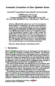
For performance evaluation of the SAXS code, we use enzymes from the Protein Data Bank (PDB), including the 1xib molecule, which has 3052 atoms. We defer a detailed discussion of computational complexity to Section 4, but we have measured ≈ 4.7 × 10⁹ evaluations of the formula to scatter the 1xib molecule. The SAXS scattering code therefore has a significant amount of computation in which we have observed a large amount fuzzy reuse [3]. The initial version of scattering code required more than 1.5 hours to scatter the 1xib molecule. Removal of redundant code and precomputation of scattering constants resulted in a 6X improvement on a 32-bit system. Porting the code to a 64-bit system yielded another 3X improvement.
Table 1: SAXS scattering code improvements.
Scattering Intensity (Absolute)
(a) 1xib molecule, which contains 3052 atoms. 10
9
10
8
Original Code Optimized Code
107 106 105 10
4
0
0.05 0.1 0.15 Scattering Angle (Radians)
0.2
(b) Original and optimized scattering curves. Figure 1: 1xib molecule and scattering curves. The project goal was to scatter thousands of rotations of various molecules. This raised the performance requirement, so we decided to investigate LUT methods. Table optimizations date back to the early days of computing [4], and are commonly used to optimize function evaluation in hardware. Programmers often use LUT methods, but the technical literature is very limited with respect to a software methodology. Our initial LUT optimization was manual, so we had to empirically determine the LUT size to meet the required level of accuracy and performance. After extensive experimentation we were able to gain an additional 7X improvement. We achieved these numbers despite a modest table size of 3.2MB and average error of < 0.0014 percent. Figure 1 shows the 1xib molecule and intensity curve. Both the original and optimized curves are plotted, but the difference between them is negligible and impossible to see visually. To improve the process we developed the Mesa tool to perform error analysis and automatic generation of LUT optimization code for a broad range of scientific expressions. Mesa, described in Section 3, allows us to characterize the performance and accuracy of LUT optimizations. In addition, we parallelized the SAXS scattering loop with OpenMP, showing a further 1.8X improvement on a dualcore, and 3.6X on a quad-core system. We conclude that the benefit of LUT optimization applies equally to the par-
Run Time
Cumulative Factor
Delta Factor
Version Description
5365s 872s 279s 41s 23s 13s
1X 6X 19X 131X 233X 413X
1X 6X 3X 7X 1.8X 1.8X
Original code Removed redundancy 64-bit system and compilers Manual table optimization Parallel version, dual-core Parallel version, quad-core
allel version, that is the single core and multicore optimizations are independent and complementary for this application. Table 1 shows the progression of performance improvements for the scattering code. Current trends in computing platforms include the broad availability of multicore hardware and a decrease in memory access performance relative to processor performance. As a result, the focus in scientific computing has shifted to parallel execution and transformations that reduce the number of memory accesses on multicore systems. However, single core performance still remains important enough to justify continued study of optimizations that improve performance by eliminating redundant operations. Such optimizations must be evaluated to ensure that they remain effective when the code is parallelized, as we have done in this paper. Mesa makes the process of applying LUT optimizations to existing code less costly and more repeatable. Our contributions are as follows: (1) we show that that LUT optimizations can benefit scientific codes, (2) we present a tool for the partial automation of LUT optimization, including error analysis, and (3) we demonstrate that LUT optimization is applicable in a multicore environment. The remainder of this paper is organized as follows: Section 2 provides background information on LUT optimization, Section 3 introduces the Mesa tool, Section 4 describes case studies performed with Mesa, Section 5 gives details on error analysis, Section 6 shows related work, and Section 7 presents our conclusions.
2.
LUT APPROXIMATION
LUT optimizations represent continuous functions as sets of discrete values, with each LUT access returning a stored approximation of the original function. Increasing the number of LUT entries improves accuracy, but reduces the level of reuse that occurs when different inputs share the same LUT entry. Decreasing reuse causes an increase in the penalties associated with memory usage, notably cache misses. Thus LUT optimizations have an inherent tradeoff between accuracy and performance. In this section we define how to characterize the error introduced by LUT optimization. LUT approximations introduce error because memory limitations make it impractical to match the floating-point accuracy of the processor. IEEE floating-point standards provide accuracy of ±1.19 × 10−07 for single-precision (SP) and ±2.22 × 10⁻¹⁶ for double-precision (DP). To match this precision for an input variable with a domain [0.0, 1.0] would require a 32MB table for a float, and a 16PB table for a double. The latter is clearly out of reach for modern computers, even for limited domains. We define a LUT approximation as a function l(x) with identical parameters to the original function f (x), but less accuracy. The l(x) function performs a table lookup by di-
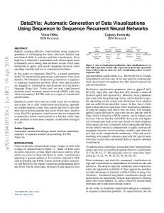
We can calculate maximum and average error statistics based on the individual errors. The maximum error is important because it bounds the error imposed on the application for a single LUT access. In the worst case, each LUT access can produce the maximum error. We define the maximum error eM AX as the largest absolute error within a LUT entry. We can combine the error terms for entries into a maximum error EM AX for the entire table by iterating over all eM AX to find the largest value. Error terms can be absolute or relative. Absolute error is the magnitude of the error term, and relative error is the error term divided by the expected value. Both representations are used in this paper, but relative errors are shown as a percentage. In the best case, a LUT access exactly matches the original function, so the minimum error is zero. The average error is therefore bounded by zero and the maximum error. If we assume a random distribution of LUT accesses within an entry, then we can compute eAV G as the arithmetic mean value of all outputs. If we assume an equal number of accesses to each LUT entry, then we can compute the average error EAV G for the table as the mean of eAV G values. The distribution of input data can vary widely, so the average error is only an approximation. The key parameter for a LUT optimization is the number of LUT entries, since accuracy increases along with LUT size. Figure 2 plots the error statistics on a log scale for the function f (x) = x2 , with a progression of LUT sizes. Graphs like the one shown can help a programmer to select a LUT size that meets the error requirements of the application. Building the graphs requires extensive computation, so fast error analysis is needed to automate LUT size selection.
3.
MESA SOFTWARE
To make the process of LUT experimentation less cumbersome, we have developed a software tool called Mesa that automatically generates LUT optimization code for expressions commonly found in scientific code. Mesa code is available for download and use under the BSD license [1].
3.1
Mesa Methodology
This section describes the workflow for applying a LUT optimization with Mesa. As previously stated, the predominant practice is to perform the steps shown below by hand. The goal of Mesa is to automate the process as much as possible, although some of steps remain manual in the current version.
5 4.5 4 3.5 3 2.5 2 1.5 1 0.5 0 100
Emax
101
102 LUT Size
103
104
(a) Maximum error
(2)
1.4
Eavg
1.2 1 LUT Error
e(x) = |l(x) − f (x)|
LUT Error
viding the input value by LUT granularity and rounding it to an integer LUT index. Each LUT entry defines an input interval that maps to a single output value. The output value for each LUT entry is computed by evaluating the expression for an input value in the interval. The ideal output value is the average of the function over the input interval. This is costly to compute so many LUT implementations simply use the value at the interval center. To evaluate accuracy, we need statistics that characterize the magnitude of the introduced error. We refer to the computation of error statistics for a LUT optimization as error analysis, described in Section 5. The most basic statistic is the error for an individual LUT access, computed as the absolute value of the difference between l(x) and f (x), as shown in Equation (2):
0.8 0.6 0.4 0.2 0 100
101
102 LUT Size
103
104
(b) Average error Figure 2: LUT error by LUT size for f (x) = x2 . 1. The first step is expression identification, which is done most effectively by manually running profiling tools. The ideal candidate expression is a computationally expensive function with high levels of fuzzy reuse, meaning that the expression is evaluated with the same approximate inputs repeatedly. Once the programmer has identified an expression, a specification file must be written for Mesa. 2. The second step is to determine domains and distributions of the input variables for the candidate expression. In some cases the input domain is easy to infer, otherwise this step require instrumentation of the target expression. The domain size is critical because it affects LUT size, and the distribution determines the level of reuse. The domain of each input variable must be included in the Mesa specification file. 3. The third step is size specification, which currently makes the user specify the LUT size on the command line. This may require multiple Mesa runs to characterize the error statistics before finding a favorable LUT size. We also have a prototype of the system that allows the user to specify a threshold for the maximum error on the command line, letting Mesa search for the smallest LUT size that keeps the maximum error within the specified value. The future direction of Mesa is automatic selection of LUT size based on error constraints and system resources.
$ c a t square . dat variable x 0.0 5.0 center ; expression x ∗ x ; $ Mesa s q u a r e . d a t o p t i m i z e d . cpp 5 e x h a u s t i v e Mesa , v e r s i o n 1 . 0 LUT o p t i m i z a t i o n s t a r t e d I n p u t Parameter : x [ 0 . 0 0 , 5 . 0 0 ] Lut s i z e : 5 A n a l y s i s method : e x h a u s t i v e Number s a m p l e s ( p e r i n t e r v a l ) : 8 388608 I n t e r v a l [ 0 . 0 0 , 1 . 0 0 ] emax : 0 . 7 5 , eavg : 0 . 2 5 I n t e r v a l [ 1 . 0 0 , 2 . 0 0 ] emax : 1 . 7 5 , eavg : 0 . 7 5 I n t e r v a l [ 2 . 0 0 , 3 . 0 0 ] emax : 2 . 7 5 , eavg : 1 . 2 5 I n t e r v a l [ 3 . 0 0 , 4 . 0 0 ] emax : 3 . 7 5 , eavg : 1 . 7 5 I n t e r v a l [ 4 . 0 0 , 5 . 0 0 ] emax : 4 . 7 5 , eavg : 2 . 2 5 Table : Emax : 4 . 7 5 , Eavg : 1 . 2 5 LUT o p t i m i z a t i o n c o m p l e t e d
Figure 3: Mesa specification file and output. 4. The fourth step is error analysis, which is fully automated in Mesa. The user invokes Mesa with commandline arguments for the specification file (input), code file (output), table size, and error analysis method. 5. The fifth step is code generation, which is fully automated in Mesa. Mesa generates LUT data or initialization code for the LUT, along with the LUT approximation function that replaces the original expression. 6. The sixth step is code integration, which requires the user to include the generated code, call the initialization and deallocation methods on entry and exit, and replace the original expression with a call to the approximation method. This introduces an extra method call that can impact performance, but the user can substitute code from the approximation function directly to avoid the call overhead. 7. The seventh step is to compare performance and accuracy. This is done by switching back and forth between the optimized and original versions of the application, comparing accuracy and performance. Accuracy can be measured as a percentage difference between the output of the original application, which is assumed to be exact, and the output of the optimized application.
3.2
Mesa Operation
The input to Mesa is a specification file containing the expression and declarations for each constant and variable used by the expression. Input variables consist of a name and a lower and upper value that defines the domain. Our expression parser handles constants, variables, math operators (+, −, ∗, /) and library functions (sin, cos, tan, sqrt, exp, log, fabs, fmod, pow). When Mesa is invoked from the command line, it parses the specification file, optionally performs error analysis, then generates LUT code. Figure 3 shows the specification file and a sample Mesa run for a LUT to optimize the function f (x) = x2 . The output shows that exhaustive error analysis was requested, resulting in display of maximum and average error terms for each entry and the entire table. Figure 4 shows the code generated by Mesa. Mesa reads expressions from the specification file and builds a 1D LUT for one independent variable or a 2D LUT for two independent variables. SP values are used for LUT data, because
0 1 2 3 4 5 6 7 8 9 10 11 12 13 14 15 16 17 18 19 20 21 22 23 24 25 26 27 28 29 30 31 32 33 34 35 36 37
// Code g e n e r a t e d by Mesa , v e r s i o n 1 . 0 // E x p r e s s i o n v a r i a b l e s f l o a t xLower = 0 . 0 0 e +00; f l o a t xUpper = 5 . 0 0 e +00; f l o a t xGran = 1 . 0 0 e +00; // O r i g i n a l E x p r e s s i o n float Original ( float x) { return ( x∗x ) ; }; // LUT Create v e c t o r l u t ; void C r e a t e ( ) { f o r ( double d=xLower ; d