4] Satish Balay, Lois Curfman McInnes, William D. Gropp, and Barry F. Smith. PETSc 2.0 users ... 8] Tony F. Chan and Barry F. Smith. Multigrid and domain ...
Mesh Component Design and Software Integration within SUMAA3d � Lori Freitagy
Mark Jonesz
Paul Plassmannx
Abstract The requirements of distributed-memory applications that use mesh management software tools are diverse, and building software that meets these requirements represents a considerable challenge. In this paper we discuss design requirements for a general, component approach for mesh management for use within the context of solving PDE applications on parallel computers. We describe recent e�orts with the SUMAA3d package motivated by a component-based approach and show how these e�orts have considerably improved both the exibility and the usability of this software.
1 Introduction
Numerical solution of a PDE-based application typically requires that the computational domain be discretized into a collection of vertices, edges, faces, and/or cells. This discretization can take a number of di�erent forms ranging from logically rectangular and multiblock structured grids to unstructured meshes consisting of simple geometric entities such as triangles or tetrahedra. Each approach has its respective strengths and weaknesses. For example, logically rectangular grids are highly e�cient in terms of computational and memory requirements, often have long-tested and trusted discretization techniques available, but are not necessarily suited for representing complex geometries. On the other hand, unstructured meshes are exible and can represent a large number of geometries, but are more computationally and memory intensive than their structured counterparts. A signi cant amount of research and development has been done to create robust software tools for the fundamental tasks associated with mesh management on distributed memory computers. These tasks range from the initial discretization of the computational domain to adaptive mesh re nement and coarsening to improvement operations such as node point smoothing and edge or face ipping. Existing tools targeted for use on distributed memory computers include Trellis [5], DAGH [17], PME [16], SUMAA3d [9], AMR++ [18], and SAMRAI [14]. In each of these cases, however, a single style The work of the rst author is supported by the Mathematical, Information, and Computational Sciences Division subprogram of the O�ce of Computational and Technology Research, U.S. Department of Energy, under Contract W-31-109-Eng-38. The work of the second author is supported by National Science Foundation grants ASC-9501583, CDA-9529459, and ASC-9411394. The work of the third author is supported by an Alfred P. Sloan research fellowship y Assistant Computer Scientist, Mathematics and Computer Science Division, Argonne National Laboratory, Argonne, Illinois. z Assistant Professor, The Bradley Department of Electrical Engineering, Virginia Tech, Blacksburg, Virginia. x Assistant Professor, Department of Computer Science and Engineering, The Pennsylvania State University, College Station, Pennsylvania. �
2 of mesh is supported, and the application interface varies dramatically among the packages. Therefore, experimentation with di�erent discretization schemes, mesh types, and re nement/coarsening schemes is often di�cult and, in many cases, requires signi cant revision of an application code. One solution for facilitating this kind of experimentation is the design of a componentbased framework for the solution of PDE applications. Such frameworks allow the application scientist to interact with a variety of software tools that are framework compliant without changing the basic interface to the application code. Active research projects which support the solution of PDEs using a framework approach include PAWS [6], POET [3], PSEware [2] and ALICE [1]. Recent e�orts to coordinate this work have been initiated through the Common Components Architecture design group. A critical aspect of this e�ort is the appropriate de nition of a component that focuses on mesh computations and interactions. This component must accommodate a diverse range of interactions because many of the fundamental tasks associated with PDE solution rely on the mesh in some manner. The de nition of this component is further complicated by the need for dynamic operations performed on the mesh itself, including adaptive re nement and coarsening and operations that improve mesh quality. Finally, the component de nition must be general enough to handle the wide variety of mesh types desired by application scientists. In x2 we describe general design requirements for a mesh component that is targeted for use on distributed-memory parallel computers. Much of our knowledge pertaining to mesh component design stems from our software development e�ort within the the SUMAA3d (Scalable Unstructured Mesh Algorithms and Applications in 3d) project. The SUMAA3d software library is an MPI-based implementation of a collection of scalable, parallel algorithms for the fundamental tasks of unstructured mesh computation [9]. These tasks include mesh generation [7], adaptive mesh re nement [13], mesh optimization [10], and mesh partitioning. In recent e�orts, we have started to address the need for component-style interactions within SUMAA3d. In this article, we describe the interfaces between SUMAA3d and solver packages such as the Portable Extensible Toolkit for Scienti c Computing (PETSc) [4] and between SUMAA3d and interactive visualization tools. For e�ciency reasons, these e�orts focus on one-to-one interactions between SUMAA3d and other software systems, but the lessons learns from these tasks form the basis for our design of a general mesh component. The interface details are given in x3. Finally, we conclude in x4 with a discussion of our future plans in this area.
2 Mesh Management as a Framework Component
The design of a framework component that can e�ciently represent many di�erent mesh styles and allow application specialists and other components general access to mesh information is quite challenging. We start by formally de ning a mesh and a component and follow with a discussion of the requirements a mesh component must meet to support a framework targeting the parallel solution of PDE-based applications. We de ne a mesh as follows. A mesh is a discrete representation of a spatial domain consisting of a collection of basic physical entities: vertices, edges, faces, and cells, each of which can be uniquely identi ed and whose relationship to each other is given by hierarchical and connectivity information. Definition 2.1.
3 By this de nition, a mesh is a purely geometric entity, and no assumptions are made about the discretizations and solution techniques used by the application scientist. To ensure maximum exibility, each of the basic mesh entities should accept a user-de ned, application-speci c data structure. Our de nition of a software component is based on the de nition given in the book Component Software: Beyond Object-Oriented Programming [19]. We note that there are many de nitions for a software component which vary slightly in substance and form, but for the purposes of the discussion in this paper, we use the following. A software component is a unit of independent deployment, separated from its environment and other components, that provides services and information through a set of well-de ned interfaces whose prerequisites and results are clearly speci ed. Definition 2.2.
Thus, a component is de ned by the information it provides, the interface or API through which interactions with other components and software occur, and its expected behavior during those interactions. To enable the independence of component developers and of the framework from any particular component instantiation, component de nition requires both an abstracted view of the interactions and a set of formal rules, or contract, for each interaction. That is, we must de ne the preconditions that are necessary for successful interaction and provide a guarantee of the postconditions of the interaction, including any actions that must be taken based on the result of the interaction. Based on De nitions 2.1 and 2.2, we can de ne a mesh component by (1) examining the steps in PDE solution process, (2) understanding and abstracting the role a mesh plays in each, (3) de ning the pre- and postconditions that must exist for each interaction to be successful, and (4) creating the appropriate interfaces that allow the interactions to take place. To illustrate this process within a speci c example, we present in Figure 1 an outline for an adaptive mesh re nement algorithm to obtain a solution to a steady-state PDE that satis es a speci ed error tolerance. Actions that change the mesh are highlighted in bold; actions that require interaction with the mesh but do not change it are italicized. In this example the mesh must interact with components designed for the italicized tasks and application-speci c routines. For each of these components we give the prerequisites (or input) required from the mesh and application, the action of the component (or output), and the expected action, if any, required of the mesh component upon completion of the interaction. Partitioning Component: 1. Input: the graph to be partitioned consisting of the basic mesh entities and their connectivity or the geometric location of the entities to be partitioned, the weighting of those entities, machine-speci c information such as number of processors, processor speed, and bandwidth 2. Output: an assignment of entities to processors, most likely in the form of an array of integers 3. Required Action: the mesh must distribute itself and any user data associated with its basic entities as decreed
4
Initialize the mesh Partition and distribute the initial mesh
Discretize the PDE Assemble and solve the algebraic system Estimate the error in the solution While the error is greater than some tolerance Re ne the mesh Partition and distribute the re ned mesh Discretize the PDE Assemble and solve the algebraic system Estimate the error in the solution EndWhile Visualize the solution General solution procedure for steady-state, adaptive PDE solution showing the actions that change the mesh highlighted in bold and the actions that require interaction with the mesh but do not change it in italics Fig. 1.
Discretization Component:
1.
Input:
basic mesh entities and associated user-de ned data structures and mesh entity connectivity; for example a nite element discretization would require mesh cells and cell vertices. In addition, discretization depends heavily on the equations being solved and may be computed by user software. 2. Output: a local approximation of the PDE and unknowns in array form. These are derived from the user-de ned data structures, and a mapping from the user data structure to the local matrix form is necessary for distribution of the solution back to the mesh. Other output includes the global ids of the mesh entities containing unknowns as well as the connectivity between mesh entities. 3. Required Action: the mesh entity must create and store a local mapping between the user's data structures and the local discretization matrix Solver Component: 1. Input: assembly of the algebraic system requires the local matrix output from the discretization component and a mapping from the mesh entities' global ids to the corresponding components in the algebraic system 2. Output: typically a vector containing the approximate solution at this step 3. Required Action: the mesh must create a global mapping that relates the global ids of the mesh entities to their location in the solution vector. The mesh must perform a scatter of the solution vector back to user-de ned data structures on mesh entities using the global mapping de ned by the solver and the mesh and the local discretization mapping Re nement Component:
5 1.
Input: basic mesh entities, associated user data, and the user software necessary to
locally estimate the error in the solution at those entities 2. Output: an array of tags indicating which mesh entities should be re ned or coarsened 3. Required Action: the mesh should create and delete entities as speci ed Visualization Component: 1. Input: scalar and vector elds derived from user data at a subset of mesh entities, geometric information from the mesh regarding the location of that data, perhaps a background coarsening function provided by the user to de ne point density in the visualization 2. Output: reduced data sets such as isosurfaces and contour planes suitable for visualization 3. Required Action: the mesh must be able to coarsen itself according to a background function describing the desired distribution of point density for visualization. The mesh should also be able to interpolate data to any point in the domain. Thus, to satisfy the contracts given in this framework example, a mesh component must meet the following design requirements. � The mesh must be able to provide lists of the basic mesh entities, geometric information about each entity, connectivity information between entities, and the hierarchical relationship between mesh entities. � Each basic mesh entity must be able to accept a user-de ned, application-speci c data structure, a processor assignment generated by a partitioning component, and re nement/coarsening tags for adaptive solution procedures. � The mesh must be able to distribute itself and the user data associated with its basic entities to processors of a distributed-memory machine. This capability implies that it can pack messages with geometric information about itself and accept and use a function for packing the user-de ned data associated with mesh entities. The mesh must have some method for handling re nement of mesh entities, including techniques for handling propagation of re nement on distributed-memory architectures. The mesh must be able to create and store mappings from the user de ned mesh entities to local discretization matrices and from the global ids of mesh entities to the corresponding location in the solution matrix and vector. The mesh must be able to accept a coarsening function as input from the visualization routine and provide data to the user as requested. Note that these design requirements make no assumptions about what geometric information in the mesh is explicitly stored. For example, a logically regular or Cartesian grid need explicitly store only a list of vertices; the other basic entities and the relationship between them can be easily derived by the ordering of the vertex storage. On the other hand, unstructured meshes have no such implicit ordering; and complete hierarchical information that relates vertices to edges, edges to faces, and faces to cell, as well as connectivity information such as neighboring element information, must be explicitly stored in the mesh
6 represtation. Thus, each instantiation of a mesh can e�ciently use computer resources by storing only the necessary information to de ne (or derive) the complete list of basic entities and relational information. Performance of a general mesh component that is capable of supporting all of the di�erent mesh styles is likely to be low. An intermediate approach that focuses on the most commonly used styles of mesh and the corresponding discretizations is likely to obtain better performance and also to satisfy most application user needs. In particular, one approach would be to provide two sets of mesh component interfaces; one that targets logically regular grids using nite di�erence discretization schemes and another that targets unstructured meshes using nite element and nite volume schemes.
3 Component Implementation within SUMAA3d
The SUMAA3d software currently handles tasks associated with instantiations of the mesh, discretization, and partitioning components described in the preceding section. In this section we describe the interface design between SUMAA3d and application-speci c code and also between SUMAA3d and the remaining two components, the solver and the visualization components. Our work to date has focused on developing particular interfaces between SUMAA3d and other software systems. In particular, subsection 3.1.1 discusses the interface between SUMAA3d and two packages for solving simultaneous systems of equations, BlockSolve95 and PETSc and subsection 3.1.2 describes the interaction between SUMAA3d and interactive visualization/computational steering software. Although not as general as the component approach described in the preceding section, this approach provides the best performance for application scientists. Future work at Argonne includes the development of the interface routines for both the general mesh case and the intermediate approach described in the preceding section.
3.1 The SUMAA3d User Interface
The interaction between a user and the SUMAA3d programming environment is based on the speci cation of a number of key properties of the application. These properties usually include the underlying governing equations, typically a (local) PDE, the problem domain, its geometry and topology, boundary conditions, and a discretization scheme for the PDE (for example, a rst-order nite-element method with particular choices for element types, quadrature rules, and error estimation schemes). A key observation is that for most applications, such as nite-element approaches, the user can specify a problem with a routine to evaluate an element (given the element data), an error estimation routine (using the data from an element and perhaps some neighborhood), and a compact representation of the computational domain (possibly a coarse surface triangulation and explicit or implicit functions to generate new surface points during mesh re nement). These operations are local and require information only from a particular element and its neighborhood. Thus, the only software required from the user should be routines for these local operations, that is element routines, error estimation routines, and surface interpolation routines. The programming interface presented by SUMAA3d is independent of underlying distributed data structures, enabling users to concentrate solely on numerical aspects of modeling. In Figure 2 we schematically show the interaction between the user and the essential components within the programming environment. The dotted line at the top of the gure denotes the user interface to the SUMAA3d programming environment. Note that
7 Geometric Description & Boundary Conditions
Mesh Generation
Error Estimation
Mesh Improvement - Refinement - Face Swapping -Vertex Smoothing
Mesh Partitioning
FE Subroutine
Matrix Assembly Κ=
Σ Ke
Sparse Matrix Solution
Ku = f
Interactive Visualization Fig. 2. A schematic of the interaction between the essential tasks required in the programming environment. This schematic illustrates how the user-supplied code (the routines represented by the ovals above the dotted line) is independent of the distributed data structures inherent to the parallel programming environment. The distributed data structures are used in parallel computations done by the essential tasks (represented by boxes below the dotted line).
the user-supplied code is independent of the underlying distributed data structures inherent in the parallel system. However, a user can access information from the distributed data structures as required to integrate other software systems. This interface not only simpli es work for the user, but also enables us to more easily interface to PETSc (as discussed in the following section), ALICE, and other related projects. 3.1.1 Interaction between Solver Packages and SUMAA3d The rst solver package interfaced to SUMAA3d was BlockSolve95 [11] [12], software for solving systems of linear equations arising from discretizations of PDEs on structured or unstructured grids. SUMAA3d makes extensive use of features and data structures speci c to BlockSolve95 to allow for e�cient matrix assembly as well as a low-overhead interface between the solver and the SUMAA3d. One such feature is BlockSolve95's tolerance of a noncontiguous global numbering of unknowns [12]; this feature allows for unknowns to be assigned a permanent global number that does not change when mesh vertices are added and deleted. The interface between SUMAA3d and BlockSolve95 is extremely e�cient, but the tight coupling of data structures and features speci c to BlockSolve95 does not satisfy the de nition of a component-based approach given in x2. The second solver package interfaced to SUMAA3d was PETSc, a exible package for solving linear and nonlinear systems of equations with the capability of solving timedependent problems [4]. PETSc is a much more comprehensive, general package than BlockSolve95; it does not have some of the features that were taken advantage of in the interface of SUMAA3d to BlockSolve95. The interface points between the two packages are the PETSc matrix and vector objects, Mat and Vec, respectively. A high-level description of the actions required by the two packages is given in Figure 3. One direction is fairly straightforward: SUMAA3d must assemble matrices and vectors into the Mat and Vec objects using the assembly routines provided by PETSc. The user calls a SUMAA3d
8 subroutine to initiate matrix or vector assembly; the user must indicate which set of unknowns is to be used in the assembly. Given this information, SUMAA3d creates and stores a mapping of the mesh unknowns to the unknowns represented in the matrix and solution vector. SUMAA3d uses this mapping to scatter the data in a PETSc Vec object onto the mesh so that the unknowns in the Vec object are mapped to the correct unknowns at the mesh vertices. Such a scattering is likely to take place, for example, after a set of linear systems are solved, and the results need to be mapped onto the mesh for further calculations. The mapping created by SUMAA3d is not used in PETSc and is not explicitly expressed to PETSc. We do, however, take advantage of the PETSc \container" software construct that allows non-PETSc data be attached to PETSc objects. We place a pointer to the mapping object in the container, and associate this container with either a PETSc Vec or a PETSc Mat object. PETSc ignores this container, but whenever SUMAA3d examines a PETSc Vec or Mat object, it looks in this container for the mapping data associated with that object. This approach allowed for the implementation of an interface between SUMAA3d and PETSc to be written without altering a single line of code of either package. Further, only a few hundred lines of new code were needed for the interface with the majority of this code associated with matrix assembly and altering matrices to enforce boundary conditions. PETSc
SUMAA3d Create vectors Xold and Xnew (type Vec)
Solve A*Xdelta=Xold
Assemble Xold from mesh Create matrix A (type Mat)
Xnew = Xdelta+Xold Assemble A from mesh Scatter Xnew onto mesh
Fig. 3. SUMAA3d is responsible for creating the PETSc objects of type Vec and type Mat that will be used by SUMAA3d. These objects use the container feature of PETSc objects to retain information describing the mapping between mesh unknowns and matrix/vector unknowns. In this example, SUMAA3d creates vectors Xold and Xnew as well as matrix A; Xold and A are assembled. PETSc solves for Xdelta, which is a PETSc Vec object that is not used by SUMAA3d, and then computes Xnew. Finally Xnew is scattered back onto the mesh by SUMAA3d using the mapping information contained in the Vec object.
3.1.2 Interactive Visualization Tools and SUMAA3d The interface between the
equation solvers and SUMAA3d was fairly straightforward in large part because there is a consensus about what algebraic operations and objects are in equations solvers, particularly for linear equation solvers. Unfortunately, the nature of the operations and implementations for interactive visualization and computational steering on unstructured meshes is still a research topic; no strong consensus exists. An important focus area is the reduction of data sent to the visualization engine.
9 Because SUMAA3d is targeted to large-scale parallel machines, the meshes are expected to have millions of unknowns and perhaps thousands of time steps. It is neither practical nor desirable to send this amount of data to a visualization engine for two reasons: (1) the computation load on the visualization engine is too high, and (2) the user does not want to and cannot look at that amount of information. E�cient operation dictates a reduction in the amount of information sent to the visualization engine. The approach advocated in this paper is the use of mesh coarsening techniques to reduce the data in space and splines to reduce the data in time. Both of these mesh functions can signi cantly reduce the amount of data to a manageable level in a controlled fashion. Mesh coarsening is typically used to construct a coarse mesh for a multilevel solver algorithm [8] where the goal is simply to construct a mesh that meets certainly quality bounds and mesh size requirements. For interactive visualization, di�erent goals are set for the coarse mesh. For example, a user may want to see only a section of the mesh, a coarse view of the entire mesh, or details in some sections of the mesh and coarse views in other sections. The visualization software would give a background function to SUMAA3d describing the desired distribution of point density in the coarse mesh as well the desired number of points in the coarse mesh; SUMAA3d would return a coarse mesh satisfying the distribution function and number of points. Splines and related functions can be used to construct compact representations of a set of points. They can be particularly e�ective in reducing the amount of data required to represent a function while still retaining reasonable accuracy. This is especially true when the function is not changing rapidly. Such a technique is not particularly useful for unstructured meshes in the spatial domain because these meshes are typically constructed such that the estimated error is equal on each element of the mesh. However, there is signi cant potential for compression in the time domain because there are typically areas of the mesh where the function changes slowly in time and areas of the mesh where the function changes rapidly. The proposed approach uses spline-like functions to compress the unknown information at each vertex in the time domain. The visualization software will convey an acceptable error level or a desired reduction in data (both are single numbers) to SUMAA3d, and the spline-like functions will be chosen at each vertex to achieve this goal. Both techniques are computationally demanding and complex, particularly in a parallel environment. A suitable algorithm of guaranteed quality exists for mesh coarsening [15]. A task in SUMAA3d is the construction of a parallel mesh coarsening algorithm using this technique. Similarly, many strong contenders exists for the time domain compression functions. The interaction of these functions with mesh coarsening as well as measurements of their compression capability is a task in SUMAA3d.
4 Conclusion
Our recent e�orts within SUMAA3d to develop interfaces among solver packages and interactive visualization tools have considerably improved both the exibility and the usability of this software. Our experience with software interaction between particular packages has led us to develop a preliminary design for a general mesh component for use in scienti c computing applications. Our eventual goal is to support interoperability through the componentware approach championed by the Advanced Large-Scale Integrated Computational Environment (ALICE) e�ort at Argonne [1]. Our future work in this area will center around creating appropriate interfaces for the mesh component described in x2. This work will not be done in isolation, but
10 rather motivated by a team of application scientists from ongoing collaborations, and in conjunction with developers of other mesh management software and with the developers of related components. Once these interfaces are in place for SUMAA3d we will explore e�ciency and generality tradeo�s in the context of a mesh component with four levels of coupling: tight data structure-dependent coupling, as with BlockSolve95, one-to-one interfaces such as that implemented with PETSc, and the two approaches to general mesh components described at the end of x2.
References [1] Information regarding the alice project can be found at http://www.mcs.anl.gov/alice, 1998. [2] PSEware home page, July 1997. http://www.extreme.indiana.edu/pseware/about/index.html. [3] Rob Armstrong and Alex Cheung. POET (Parallel Object-oriented Environment and Toolkit) and frameworks for scienti c distributed computing. In Proceedings of HICSS97, 1997. [4] Satish Balay, Lois Curfman McInnes, William D. Gropp, and Barry F. Smith. PETSc 2.0 users manual. ANL Report ANL-95/11, Argonne National Laboratory, Argonne, Ill., November 1995. [5] Mark Beall and Mark Shephard. A geometry-based ananlysis framework. In Proceedings of ICES'97, Seattle, Washington, March, 1997. [6] Peter Beckman, Patricia Fasel, and William Humphrey. E�cient coupling of parallel applications using PAWS. In Proceedings of the High Performance Distributed Computing Conference, Chicago, IL, July, 1998. [7] Marshall W. Bern and Paul E. Plassmann. Mesh generation. In Jorg Sack and Jorge Urrutia, editors, Handbook of Computational Geometry. Elsevier Scienti c, to appear. [8] Tony F. Chan and Barry F. Smith. Multigrid and domain decomposition on unstructured grids. Electronic Transactions on Numerical Analysis, 2:171{182, 1994. [9] Lori A. Freitag, Mark T. Jones, and Paul E. Plassmann. The scalability of mesh improvement algorithms. In Michael T. Heath, Abhiram Ranade, and Robert S. Schreiber, editors, Algorithms for Parallel Processing, volume 105 of The IMA Volumes in Mathematics and Its Applications, pages 185{212. Springer-Verlag, 1998. [10] Lori A. Freitag, Mark T. Jones, and Paul E. Plassmann. A parallel algorithm for mesh smoothing. SIAM Journal on Scienti c Computing, to appear. [11] Mark T. Jones and Paul E. Plassmann. Scalable iterative solution of sparse linear systems. Parallel Computing, 20(5):753{773, May 1994. [12] Mark T. Jones and Paul E. Plassmann. BlockSolve95 users manual: Scalable library software for the parallel solution of sparse linear systems. ANL Report ANL-95/48, Argonne National Laboratory, Argonne, Ill., December 1995. [13] Mark T. Jones and Paul E. Plassmann. Parallel algorithms for adaptive mesh re nement. SIAM Journal on Scienti c Computing, 18(3):686{708, May 1997. [14] Scott Kohn, Xabier Garaizar, Rich Hornung, and Steve Smith. SAMRAI web pages, http://www.llnl.gov/CASC/SAMRAI/, 1998. [15] Gary L. Miller, Dafna Talmor, and Shang-Hua Teng. Optimal coarsening of unstructured meshes. Manuscript, 1997. [16] Can Ozturan. Parallel mesh environment homepage. http://www.icase.edu/newresearch/des/highlite/cs4.html, 1998. [17] Manish Parashar and James Browne. DAGH: Data-management for parallel adaptive meshre nemnt techniques. http://www.caip.rutgers.edu/ parashar/DAGH, Sep 1998. [18] D. Quinlan. AMR++: A design for parallel object-oriented adaptive mesh re nement. In Proceedings of the IMA Workshop on Structured Adaptive Mesh Re nement, Minneapolis, MN, 1997. [19] C. Szyperski. Component Software: Beyond Onject-Oriented Programming. Addison-Wesley, 1998.