Mesh-Driven Vector Field Clustering and Visualization - Department of ...

JOURNAL OF LATEX CLASS FILES, VOL. 6, NO. 1, JANUARY 2007

1

Mesh-Driven Vector Field Clustering and Visualization: An Image-Based Approach Zhenmin Peng, Edward Grundy, Robert S. Laramee, Guoning Chen, and Nick Croft Abstract—Vector field visualization techniques have evolved very rapidly over the last two decades, however, visualizing vector fields on complex boundary surfaces from computational flow dynamics (CFD) still remains a challenging task. In part, this is due to the large, unstructured, adaptive resolution characteristics of the meshes used in the modeling and simulation process. Out of the wide variety of existing flow field visualization techniques, vector field clustering algorithms offer the advantage of capturing a detailed picture of important areas of the domain while presenting a simplified view of areas of less importance. This paper presents a novel, robust, automatic vector field clustering algorithm that produces intuitive and insightful images of vector fields on large, unstructured, adaptive resolution boundary meshes from CFD. Our bottom-up, hierarchical approach is the first to combine the properties of the underlying vector field and mesh into a unified error-driven representation. The motivation behind the approach is the fact that CFD engineers may increase the resolution of model meshes according to importance. The algorithm has several advantages. Clusters are generated automatically, no surface parameterization is required, and large meshes are processed efficiently. The most suggestive and important information contained in the meshes and vector fields is preserved while less important areas are simplified in the visualization. Users can interactively control the level of detail by adjusting a range of clustering distance measure parameters. We describe two data structures to accelerate the clustering process. We also introduce novel visualizations of clusters inspired by statistical methods. We apply our method to a series of synthetic and complex, real-world CFD meshes to demonstrate the clustering algorithm results. Index Terms—Vector Field Visualization, Clustering, Feature-based, Surfaces.

F

1

I NTRODUCTION

VER the last two decades, vector field visualization has developed very rapidly. Its applications range from the automotive industry to medicine. Vector field visualization provides solutions that enable engineers to investigate and analyze critical features and characteristics of the flow from computational fluid dynamics (CFD). However, visualizing and analyzing vector fields on complex boundary surfaces from CFD still remains a challenging task due mainly to the large, unstructured, adaptive resolution characteristics of the meshes used in the modeling and simulation process (see Figure 2). Unstructured meshes necessitate either computationally expensive neighbor searching or the explicit storage of mesh topology, which, for large meshes, can cause nontrivial memory overhead. Adaptive resolution meshes cause problems with scale. Some portions of the mesh may be too fine to visualize concurrently with coarse resolution regions. Additionally, as the size of simulation datasets from CFD increases, so does the demand for visualization methods that quickly depict vector fields in a simplified and insightful manner. Finding a good solution that handles both complex

O

boundary surfaces from CFD and provides a suggestive picture of vector fields is a challenge that we address. Out of all the possible visualization techniques that can be used to simplify and present simulation results, vector field clustering algorithms are a desirable solution which offer the advantage of presenting a detailed picture of important or complex areas of the domain while depicting a simplified representation for areas of less importance. In general, clustering algorithms are based on agglomerative hierarchical grouping techniques which are widely used in the information visualization domain [1]. However, vector field clustering algorithms have received relatively little attention. In this paper, we present a novel, automatic vector field clustering algorithm that handles vector fields on complex boundary surfaces from CFD. It produces simplified but insightful images based on an error-driven distance measure.

One of the primary motivations behind our method stems from the semantics of meshes from CFD. When constructing a model, portions of the geometry which are more important may be modeled with a very fine resolution in order to obtain simulation results with higher accuracy. Constituents of a model deemed less interesting to the engineer may be • Z. Peng, E. Grundy and R.S. Laramee are with the Department of represented with a coarser resolution mesh in order to speed up Computer Science, Swansea University, SA2 8PP,Wales, United Kingdom. the simulation process. The resolution of a region of the mesh Email:[email protected],[email protected],[email protected]. can reflect the importance of that region to the engineer; thus, • G. Chen is with the Scientific Computing and Imaging Institute, University of Utah,72 S Central Campus Drive, Room 3750, Salt Lake City, UT 84112. it is an encoding of the engineers knowledge of the problem. Email:[email protected]. More than 50% of the time spent on an industry grade CFD • N. Croft is with the School of Engineering, Swansea University, SA2 process (meshing, simulation, and visualization) is devoted to 8PP,Wales, United Kingdom. Email:[email protected]. defining and generating the mesh [5]. The mesh resolution can also depend on the size of the individual components

JOURNAL OF LATEX CLASS FILES, VOL. 6, NO. 1, JANUARY 2007

2

Fig. 1.

The visualization of flow at the stream surface of a gas engine simulation [2], [3]. (left) The stream surface mesh is composed of unstructured, adaptive-resolution polygons. For stream surface generation, we use the algorithm of Garth et al. [4] which handles unstructured, adaptive resolution meshes. (middle-left) Clusters rendered with by ε = 15%. The comparison of glyphbased hedgehog visualization (middle-right) and cluster-based streamlet visualization with semi-transparent clusters (right). Here we can visualize vector field clusters on stream surfaces for the first time. The color of glyphs (middle-right) and streamlets (right) is mapped to velocity magnitude.

found within the model itself. Very small constituents of the geometry are treated with detailed, high resolution meshes. Larger features are modeled with a coarser resolution. Our clustering algorithm and resulting visualization takes both the semantics of the underlying mesh and the characteristics of the vector field into account. The main benefits and contributions of this method are: • A novel clustering algorithm which couples the properties of the vector field and mesh model into a unified clustering distance measure. The model and implementation are general enough such that any arbitrary attribute of the CFD simulation results may be incorporated into the clustering distance measure. • A cluster hierarchy is generated automatically according to the importance of the underlying mesh and the properties of the vector fields. More detailed areas are emphasized while less important or simpler ones are simplified in a single image. • Large, adaptive resolution meshes are handled efficiently because clusters are never generated for occluded or otherwise invisible regions of vector fields on the surfaces. • We introduce novel visualizations of cluster attributes including θ -range and |v|-range glyphs. Our approach enables various clustering and visualization resolutions, optimized for either speed or accuracy. The approach enables a range of user-controlled visualization parameters such as automatic glyph and streamlet placement options. Glyphs can be automatically placed at the center points of clusters. Streamlets can be seeded and traced from cluster center points to render an intuitive overview of vector fields. The algorithm is robust because it handles meshes with holes, discontinuities, and jagged edges. Furthermore, the algorithm does not rely on a parameterization of the surface. The key to the technique’s robustness and simplicity is its image space approach. However, in order to achieve these benefits several challenges, both technical and perceptual, must

be overcome. The rest of the paper is organized as follows: Section 2 provides an overview of related research work. The algorithm and user options are described in multiple stages in Section 3. Section 3 also describes two important data structures used to simplify and accelerate the process. Section 4 gives the performance and visualization results. Conclusions and suggestions for future work are presented in Section 5.

2

R ELATED W ORK

Xu and Wunsch II [1] present a comprehensive and systematic survey focused on scalar clustering algorithms rooted in statistics, computer science, and machine learning. They generalize the clustering analysis procedure using four steps: feature selection or extraction, clustering algorithm design (or selection), cluster validation, and result interpretation, they detail clustering algorithms in terms of the nature of clusters. To compare different clustering algorithms, applications to some benchmark data sets are presented. Clustering algorithms can be divided into two groups: either based on constructing a hierarchical structure or based on partitioning into a collection of disjoint sets. Hierarchical clustering algorithms are mainly classified as agglomerative methods and divisive. Since the agglomerative methods can generate flexible clustering using binary trees and provide very informative descriptions, they are employed to develop some vector field clustering visualizations, such as Telea and Van Wijk [6] and Heckel et al. [7]. The computational cost for hierarchical clustering can be expensive (e.g. O(N 2 ) where N is the number of data samples.) so some of the early hierarchical clustering methods are not capable of handling large-scale data sets. To address this problem, some efficient hierarchical clustering methods are introduced like BIRCH [8] which utilizes the clustering feature tree to improve the robustness and reduce the computational complexity to O(N).

JOURNAL OF LATEX CLASS FILES, VOL. 6, NO. 1, JANUARY 2007

Fig. 2. The unstructured adaptive resolution boundary grid of a cooling jacket from a CFD simulation. The upper image is an overview of the boundary mesh, and the bottom is a close-up. These images illustrate how complex a typical mesh from CFD can be. The finest mesh resolution is used at the gasket between the cylinder block (bottom) and the cylinder head (upper component half). The gasket is modeled with the finest resolution mesh because the gasket holes are very small with high curvature. Polygons in this mesh differ in size by six orders of magnitude. There have been very few previous clustering methods targeted at vector fields, especially when compared to the large volume of flow visualization literature in general [9], [10], [11]. Telea and Van Wijk [6] present a hierarchical clustering method which automatically places a limited number of glyphs in a suggestive manner to represent the vector field. It is the first algorithm of its kind and produces both global and local information in the same image. In terms of the clustering algorithm, two candidate clusters are selected and merged together in a bottom-up fashion. During this process, a similarity measure is used to evaluate which clusters should be merged. An error measure based on local vector magnitude and direction is introduced to define how a new cluster is merged

3

from two existing ones. Heckel et al. [7] present a method to visualize discrete vector fields in a hierarchical fashion. This method uses a clustering approach to segment the original vector field into a series of disjoint clusters. The algorithm is applied in a topdown fashion. Firstly, points from the original vector field data are treated as a single cluster. Then a procedure of splitting clusters is applied using a weighted best-fit plane which partitions the space into convex regions (sub-clusters). Each region has an error measure which calculates the differences between the original discrete vector field and the simplified vector field. With the use of the error measure approach, the recursive procedure of splitting clusters can be terminated when a user-defined threshold value is met. This method is free of discretization introduced by a regular grid or sub-sampling for multi-resolution analysis. Garcke et al. [12] present a multiscale method for vector field clustering in 2D and 3D space. This continuous clustering method is inspired from the well-known physical phase separation clustering model - the Cahn-Hilliard model [13]. In order to classify and enhance the correlation in the cluster sets effectively, this phase-separation-based continuous clustering method formulates the clustering problem as a diffusion problem rather than a merging or a splitting problem. In accordance with the underlying physical data and based on the evolution function, segments of the flow field are extracted and classified depending on their location and orientation. Then, a skeletonization approach is applied to highlight the essential features of the refined cluster sets. Finally, various geometric representations are adopted to render the highlighted skeleton in an intuitive way. All the results feature uniform resolution, rectilinear grids. Griebel et al. [14] present a vector field clustering method based on algebraic multigrid [15]. Each sample in the flow field is represented by a tensor stiffness matrix that encodes the local properties of the flow field. The algebraic multigrid technique operates on these tensor matrices in order to construct a vector field hierarchy which describes the flow structure. The method is geometry-free and is demonstrated on 2D and 3D vector fields. Du and Wang [16] present a Centroidal Voronoi Tessellation based method for the simplification and the visualization of vector fields. In the method, the generators of the tesselation are treated as centers of the surrounding Voronoi regions which are deemed as the clusters. A distance function in both the spatial and vector space is applied to measure the distances between the center and surround clusters and thus determine the set of generators with the smallest distances as the final centers of the clusters. The proposed method is to minimize the global error function. The algorithm is demonstrated on rectilinear 2D and 3D vector fields. McKenzie et al. [17] present a global vector field clustering method as an extension to Du and Wang’s previous work [16]. By taking the direction, gradient, curl and divergence into account to drive the clustering process, this method can provide a meaningful segmentation of the input vector field. It is one of the few methods that is demonstrated on tetrahedral meshes. The semantics of the uniform resolution data are not

JOURNAL OF LATEX CLASS FILES, VOL. 6, NO. 1, JANUARY 2007

4

Fig. 3. An overview chart of our mesh-driven vector field clustering algorithm for surfaces. considered. There are several recent texture-based algorithms that visualize flow at the boundary surfaces of simulation data [18], [19], [20] including streamsurfaces [2]. However, texturebased methods are different class of visualization techniques from vector field clustering with different characteristics. Firstly, texture-based methods treat the flow uniformly. The resolution of the textures is generally constant. The one exception is that of Telea and Strzodka[21]. Secondly, texturebased methods fail to depict the downstream direction of the flow in a still image. Users must rely on animations of the flow for visualizing the downstream direction. Thirdly texture-based methods do not reflect the semantics of the underlying mesh in the resulting visualization. For a survey of texture-based methods see Laramee et al. [9]. Another class of flow visualization techniques focuses on the topology of the vector field [22], [23], [24]. Topological methods do not depict the downstream direction of the flow in a still image. They generally rely on another visualization method to do so. Furthermore, topological methods present challenges with respect to interpretation. Only specialists will fully understand the information conveyed by a topological skeleton of the flow. This class of methods also ignores the semantics of the underlying mesh. Visualization of the topological skeleton of the flow is not the goal of the work presented here. If a user would like to visualize the topological skeleton of a vector field, we recommend an algorithm tailored specifically to do so [25], [26]. The method here, on the other hand, generates both detailed and summary information in the same visualization. See Laramee et al. for a overview of topology-based approaches [22]. To our knowledge the algorithm we present is the first vector field clustering method that takes the properties of the underlying mesh into account in addition to the underlying vector field. This is also the first of its kind to target surfaces from CFD and to handle large, unstructured, adaptive resolution meshes efficiently. In general, previous work deals with data on structured grids.

Fig. 4. Here are 5 constituent images, plus a 6th final image, used for the visualization of surface flow on a gas engine: (top, left) the initial adaptive resolution mesh, (top, right) a velocity magnitude color mapped image, (middle,left) the attribute image corresponding to the vector field and underlying mesh resolution, (middle, right) a color mapped image which shows the different resulting clusters, (bottom, left) an image overlay, (bottom, right) the final visualization using glyphs, and the image overlay. Color is mapped to velocity magnitude. The tumble motion depicted in the lower-right image is consistent with previous visualization of the same data [3].

3

M ESH -D RIVEN V ECTOR F IELD C LUSTER ING FOR S URFACES In this section, we present details of the our algorithm including both the model and its implementation. 3.1 Method Overview Figure 3 shows an overview of our method. The input includes a generic triangular mesh as a geometric representation for boundary meshes. Each vertex i has a position ri = (rix , riy , riz ), a normal vector ni = (nix , niy , niz ), a velocity vector vi = (vix , viy , viz ) and the neighboring topology. For simplicity we assume that the velocity is confined to the surface (possibly by projection), i.e. vi · ni = 0. Note that any CFD simulation attribute can be stored at the vertices such as temperature, pressure, kinetic energy etc. This is also true of derived attributes like gradients and mesh resolution as described in Section 3.2.

JOURNAL OF LATEX CLASS FILES, VOL. 6, NO. 1, JANUARY 2007

Fig. 5. A composition of 6 triangles which share a common vertex i represents a 1-Ring neighborhood of the underlying mesh from which a local resolution measure is derived.

A mesh resolution measure, m, is computed at each vertex in a pre-processing phase. Step two is to construct an attribute image. The attribute image is a data structure which holds a simplified view of the model’s data attributes including the vector field and the quantified mesh resolution. In order to generate a simplified representation of vector fields for surfaces, a bottom-up hierarchical clustering is applied to the data using a distance measure which includes a local description of the mesh. Then glyphs or streamlets are placed automatically based on the user-defined error measure along with the original surface geometry. Additionally, various enhancements and user options, like distance measure weighting coefficients, can be used to customize the clustering process and thus the final visualization result. An overview of this process is depicted in Figures 3 and 4. It’s also worth mentioning that if the viewpoint is changed after the final visualization rendering, the next pass will start from the attribute image construction. Starting with the hierarchical clustering if the clustering distance measure parameters are changed, only a subset of the algorithm is required. Details are given in the sub-sections that follow. One consequence of storing the clusters in a list is the implicit ordering of hierarchy construction. In clustering terminology, the choice of seed clusters affects the result. The fact that the choice of seeds changes the result is a property inherent to many clustering algorithms [1], not just the one presented here. In our algorithm, seeds are always processed in the same order, from the top-left to the bottom-right in a rasterized fashion. 3.2

Mesh Resolution Derivation

Meshes from CFD data sets are adaptive resolution meshes generated according to the importance of constituents in the model. Components of the geometry requiring more accurate simulation results, such as the gaskets of Figure 2 and the intake port of Figure 4, are modeled with a dense resolution mesh. Some features are considered less important, like the cylinder block (Figure 4), and are modeled with a coarse resolution mesh for fast computation. The semantics of the underlying mesh are an important characteristic and can be incorporated into the clustering algorithm along with characteristics of the vector field. We define the resolution of the mesh around a vertex, v, as the density of triangles composed of v and two other vertices. The higher the resolution of the mesh, the smaller the corresponding polygons and thus the shorter the polygonal edge lengths. To derive a resolution measure, we use the length of edges in a 1-Ring neighborhood. We use a vertex-centered

5

edge mean function as a preprocessing stage of our clustering algorithm. Each vertex, i, in the mesh has a given set of edges, en , in a 1-Ring neighborhood as depicted in Figure 5. The mean length is computed from this set of edges. The resulting mean length eavg represents the resolution of the local neighborhood around i and is stored as a derived attribute at each vertex in the data set. eavg =

1 i=n ∑ ei n + 1 i=0

(1)

The resolution in this local region of the mesh is approximated 1 by m = . Note that this is not the only way to calculate eavg a resolution measure for the underlying mesh and that this is only an approximation. There are other options, such as an area-based mean function or computing the density of vertices per unit area.

3.3

Attribute Image Construction

The mesh resolution mi is stored at each vertex, i, of the polygonal CFD mesh along with vi . A key step is to project these attributes defined at the boundary surface to the image plane. We encode the object-space vector field, (vix , viy , viz ), and the object-space mesh resolution, (m), of each vertex into the R, G, B, and α components of a high precision texture. The formula to encode the components is: Ci =

vi − min(vi ) where Ci = (CR ,CG ,CB ) max(vi ) − min(vi )

(2)

The formula for encoding the object-space mesh resolution is: mi =

emin · (emax − eavg (i)) eavg (i) · (emax − emin )

(3)

Where emax > emin . Encoding mesh attributes in this way yields the following benefits: •

• • •

•

Occluded or otherwise hidden portions of the geometry are automatically filtered out and eliminated from any further processing. The input to the clustering algorithm is projected from an unstructured mesh to a uniform, rectilinear grid. Interpolation of vector components and the mesh resolution is performed automatically by the graphics hardware. No more computation time is spent on polygons whose size is less than one pixel, the occurrence of which is high for CFD meshes (see Figure 2). The complexity of vector field clustering in object space is reduced to a much simpler problem in image space.

After the encoding of the vector field and mesh resolution, an attribute image is rendered. Note that high-precision (RGBA 32F ARB) textures can be used to limit quantization and prevent clamping. The attribute image is used as the input to the clustering procedure (not for visualization purposes). A sample attribute image is shown in Figure 4 (middle, left).

JOURNAL OF LATEX CLASS FILES, VOL. 6, NO. 1, JANUARY 2007

6

Fig. 7. An example illustrates the clustering method. It starts with a given cluster, A, and a cluster list L(ψ) which stores the initial leaf clusters for the hierarchical clustering process. After the search process is finished, a new cluster, cluster G, is formed from two child clusters, A and D, which have the shortest distance ε (ψA − ψN ). G is added to the back of L(ψ). The corresponding binary tree is updated to store the new parent cluster and its children. 3.4

Projection and Decoding

Following the construction of the attribute image, the projection of the attributes defined at the surface is done by the graphics hardware during the rasterization stage. Since the vector components vi and mesh resolution mi are stored in the framebuffer, projected values can be decoded from the framebuffer with: vi = Ci · (max(vi ) − min(vi )) + min(vi ) eavg (i) =

emin · emax emax · mi − emin · mi + emin

(4) (5)

Where emin > 0.0. These decoded values are used to reconstruct the required field attributes as input to our clustering algorithm. Interpolation of the attribute image is necessary for reconstruction. By using hardware-assisted interpolation, we can decode mesh attributes within the original boundary mesh polygons in addition to the information stored at the vertices. See Figure 4 for an example. 3.5

Hierarchical Clustering

For a simplified representation of vector fields at surfaces, a bottom-up hierarchical clustering method is applied to the attribute image using a unified clustering distance measure that includes a local description of the mesh. 3.5.1 A Mesh-Driven Vector Field Clustering Measure To quantify the similarity (or difference) of the characteristics of different clusters, a clustering distance measure is needed. In our clustering algorithm, a clustering error measure is applied to quantify the local characteristics of the vector field and the local description of the mesh. A cluster, ψ, is defined as a five-tuple: ψ(r, v, α, m, ε) where r is the center-point of the cluster, v is the mean velocity magnitude, α is the mean velocity direction, m is the mean mesh resolution, and ε is the local clustering error. We formulate the distance between clusters with the following measure: ε (ψ) = cd ·

d dmax

+ cv ·

v vmax

+ cα ·

α m + cm · αmax mmax

(6)

where cd + cv + cα + cm = 1.0. The components of the error measure are: • Euclidean Distance (d): this constituent measures distance between two cluster centers, ψA , ψB using d = |ψAr − ψBr |. This component encourages the clustering algorithm to group clusters whose centers are in close proximity. See Figure 6 (upper-middle, left). The Euclidean distance between two points in 3D space can be computed using a combination of (x, y) image space coordinates and information from the depth buffer for the (z) component (see Section 3.5.3). The maximum distance, dmax , is the length of a diagonal for the geometry’s bounding box. It groups clusters visually. • Velocity Magnitude (v): this constituent measures the difference between the mean velocity magnitude of two clusters, ψA , ψB using v = ψAv − ψBv . This component encourages the clustering algorithm to group the clusters which have similar magnitude. See Figure 6 (uppermiddle, right). The maximum velocity, vmax , is the largest magnitude of the given data set. • Direction (α): this constituent compares the velocity direction of two clusters, ψA , ψB using α = ψAα − ψBα . It drives the clustering algorithm to group the clusters which have similar direction. See Figure 6 (lower-middle, left). The maximum direction value, αmax , is 180°. • Mesh Resolution (m): this component differs from the other three. Rather than comparing the vector field features, it sums the resolution of the local mesh from two clusters, ψA , ψB using m = ψAm + ψBm . The effect of this measure is to accumulate error proportional to the local density and thus present the user with a more detailed representation in regions with a denser mesh. In other words, multiple, shorter edges accumulate more error than a single long straight edge, thus for a given ε, clusters in high resolution mesh regions are generally smaller. See Figure 6 (lower-middle, right). The maximum mesh resolution, mmax , is the largest value of m derived in Section 3.2. • Local Error(ε): this is not used as part as the distance clustering measure but is simply the result stored from the previous pairing of two clusters and represents the

JOURNAL OF LATEX CLASS FILES, VOL. 6, NO. 1, JANUARY 2007

7

clustering distance measure. The fully automatic version of the algorithm essentially ignores the weighting coefficients thus minimizing the need for interaction. These components may be treated independent from one another. By changing the weighting coefficients different distance measures can be tailored to address the user’s needs. The effect of varying these coefficients is shown in Figure 6. We note that adjusting cd , cv , cα , and cm is optional. Their values are set to 25% by default throughout this paper unless noted otherwise. Modifying coefficients is user-dependent. The distance measure is the key that drives the algorithm and produces a suggestive and simplified depiction of the vector field on surfaces. See the combined clustering result in Figure 6 (lower, left) and also the final visualization (lower, right). The larger glyphs indicate areas of more uniform flow. The same saddle point and vortex visualized in the lower-right of Figure 6 is consistent with previous work [27]. The cluster geometry is stored as a list of pixels and their edges. The center of a cluster is simply the average position of each pixel center. If the user would like more control over the shape of the clusters in order to avoid U-shaped clusters for example, then cd in equation (6) may be increased. The effect of increasing cd is shown in Figure 6. Users interested in regions of similar velocity magnitude increase cv . Users interested in seeing features such as sources, sinks, and saddle points increase cα . Users who would like more detail in areas of high mesh resolution increase cm .

Fig. 6. Constituent images from the result of clustering process driven by the error measure, used for the visualization of surface flow on a gas engine: (top, left) the initial adaptive resolution mesh, (top, right) a velocity magnitude color mapped image, (upper-middle, left) the result of clustering process by setting cd = 100%, (upper-middle, right) the result from setting cv = 100%, (lower-middle, left) the result of cα = 100%, (lowermiddle, right) the result of cm = 100%, (bottom, left) the result by setting cd = cv = cα = cm = 25%, (bottom, right) streamlets are used to illustrate the vector field based on the attribute field clusters. Color is mapped to velocity magnitude. combined local cluster error. Each component of the distance measure, including ε, is stored in the normalized range [0, · · · , 1] in order to unify the various measures. Note ε is a measure of how well a centroid describes a region of data. Optional user-defined weighting coefficients, cd , cv , cα , cm are introduced to adjust the contribution of the first four components to the final

3.5.2 Generating the Cluster Hierarchy Our algorithm is an agglomerative, average-linking clustering process. As the basic component of the cluster hierarchy each cluster is stored as a node containing r, v, α, m, ε. Given a cluster, ψA (r, v, α, m, ε), the bottom-up, hierarchical algorithm is conceptually a search process. ψA tests its neighbors looking for a merge candidate. Neighbors share a common cluster edge. The candidate with the minimum clustering distance, |ψA − ψB |, is chosen and a new parent cluster ψAB is formed. Initially, the smallest clusters are the individual pixels of the attribute image with zero error. The clustering and tree generating process starts in the top-left corner and seeds in rasterized fashion. This process is repeated for each cluster until only one root cluster remains. Although this method is easy to apply, the computational cost becomes a problem since each cluster ψB which can be merged with a given cluster ψA needs to be tested using the distance measure. In order to accelerate the hierarchical process, we introduce another structure to speed up the candidate cluster searching process. This structure consists of a lookup table ψ LUT and a neighbor list ψ l for each cluster. The lookup table accelerates the search process essentially by a tradeoff between storage space and processing time. Instead of performing a traversal of the entire hierarchy for neighbors, the location of child nodes and parent nodes is stored and updated after each search process. ψ LUT is the same resolution as the leaf clusters and stores the address of each leaf cluster’s topmost parent cluster. ψ l stores the address of each adjacent leaf cluster. With this additional information, the candidate cluster ψB which may be grouped with the current cluster ψA to form

JOURNAL OF LATEX CLASS FILES, VOL. 6, NO. 1, JANUARY 2007

a new cluster can be located quickly. We illustrate the process using the example in Figure 7. In order to represent initial leaf clusters of the vector field in image space, a rectilinear grid, the resolution of which is defined by the user, is placed in image space. Cluster attributes are then retrieved at each grid cell using the decoding procedure described in Section 3.4. Each leaf cluster contains a neighbor list ψ l and is added onto a central cluster list L(ψ) which stores nodes for the bottom-up hierarchical clustering process. The clustering process starts from the head of the list L(ψ). Our clustering algorithm begins by traversing ψAl for the given cluster ψA . For example in Figure 7, the given cluster A searches its adjacent clusters ψAl . The ψ LUT stores topmost parent clusters for these adjacent leaf clusters and also indicates the leaf clusters which have the same top-most parent cluster in the neighbor list. A refined neighbor list which contains only the unique cluster candidates can be obtained for cluster A. ε is computed for each candidate cluster. The cluster resulting in the smallest error is chosen. In Figure 7, D is the candidate selected. Once a candidate in ψAl is selected, a new cluster, G, can be formed by grouping A and D. Meanwhile, ψGLUT is updated. The new cluster is stored in the form of a parent node whose two child nodes are A and D. G is added to L(ψ) to be processed. When L(ψ) contains only one node, the bottom-up hierarchical clustering is completed. 3.5.3 Edge and Discontinuity Detection During the clustering process, cluster ψB chosen to be grouped with ψA is found by applying the distance measure to ψAl . However, a complication can arise with this approach due to discontinuities and sharp edges on the surface. If we do not take discontinuity in the geometry into account then we may end up grouping clusters that do not belong together. To address this problem, we compare ψAdepth with ψBdepth . If εdepth < |ψAdepth −ψBdepth | then ψB is not grouped with ψA . This approach separates the image into local regions with boundaries. In practice, we have found a value of εdepth ≈ 0.3% to be a good threshold. 3.6

Image Overlay

An image overlay is used for the resulting visualization of the clustering on surfaces by applying color, shading, or any attribute mapped to color. In the implementation, we generate the image overlay following the construction of the attribute image once for each static scene. Once the view-point is changed, the image overlay is regenerated. By exploiting the glDrawPixels() function from OpengGL, rendering an image is much faster than rendering the complex 3D triangulated object each time a user parameter is changed. 3.7

General Attribute-based Clustering

Our clustering method can be extended to incorporate any general attribute of CFD simulations in the distance measure. Not only can the properties of the vector field and the

8

Fig. 8. The result of the clustering driven by an error measure (εε = 12%) which uses the depth as a distance measure constituent. Notice how the overall density is much higher towards the rear.

resolution of the underlying mesh be coupled into a unified distance measure, but also any other CFD simulation attribute can also be used to drive the clustering process such as temperature, pressure, kinetic energy and derived data such as gradients. By encoding these values into the attribute image using the method in Section 3.3 and building up the hierarchy following the scheme in Section 3.5.1, we can obtain arbitrary attribute-based clusters for different user needs. Figure 8 demonstrates the effect of using ψ depth . For demonstration, we have simply substituted mesh resolution, m, with another attribute, ψ depth = ψAdepth + ψBdepth in equation (6). In this example, regions further away from this viewer (higher depth value) are denser in the visualization. 3.8

Visualization Options

Using the binary tree, clusters can be traversed in a depth first search fashion driven by a user-defined error value. In this searching process, the (deepest) clusters where ψ ε ≤ ε are rendered for visualization. Several user options are available for the visualization of the selected clusters. 3.8.1 Color Coding and Mean Vector Glyphs A selection of colors can be blended to depict different clusters. This is shown in Figures 6, 1 (middle-left), 8, and 15. Visualization using vector glyphs is one of the most straightforward methods to visualize the flow field. In our algorithm, a mean 3D vector glyph is placed at the center of each cluster. Glyph size may be mapped to the size of the corresponding cluster while the color can be mapped to the mean velocity magnitude. See Figure 8 and 13. The user may zoom in to areas with dense glyphs for more detail. This is one way to resolve occlusion. Other ways include mapping color to mean velocity magnitude or using streamlets. 3.8.2 Streamlets Cluster-center-based streamlet seeding is another visualization option. This automatically traces a 3D streamlet tube from each cluster center until it hits the cluster boundary. The streamlet curves are traced according to the original vector field. In Figures 1 (right) and 15, a cluster-based streamlet technique (bottom) gives insightful imagery by applying

JOURNAL OF LATEX CLASS FILES, VOL. 6, NO. 1, JANUARY 2007

9

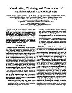
Fig. 9.

|v|-range glyphs: (Top) a close-up look at a |v|range glyph whose inner radius represents the minimum velocity magnitude while outer is mapped to the maximum. (Bottom) the result image with |v|-range glyphs applied to depict the variation in magnitude within each cluster .The result of the clustering driven by an error measure (εε = 15%). Glyph color is mapped to velocity magnitude.

streamlet depiction in the more important areas while yielding a sparse depiction in areas of less importance. Arrow heads can be added to the streamlets to indicate the downstream direction of the flow. Using arrow heads in the visualization can introduce occlusion. To eliminate this the user can disable the arrow heads leaving only streamlet curves. Color coding cluster according to velocity magnitude is also occlusion free. This is one way to resolve occlusion. Other ways include mapping color to mean velocity magnitude or using streamlets. 3.8.3

|v|-Range Glyphs

Automatically providing more detail in areas of high vector field variance and mesh resolution is deemed helpful to engineers. |v|-range glyphs are used to visualize the variation in vector field magnitude within each cluster. We use a ringlike glyph as in Figure 9 (top) where |vmin | is mapped to the inner ring and |vmax | is mapped to the outer ring. The |v|-range glyphs are placed at the center of each cluster. Regions with relatively large variation in |v| become obvious. Range glyphs (as opposed to deviation glyphs) have the advantage that they include outliers in the visualization. 3.8.4

θ -Range Glyphs:

θ -range glyphs depict the variance in vector field direction within each cluster. A semi-transparent cone-like glyph, as in Figure 10, whose radius represents the maximum range of θ from θ to θmax is used. Clusters with a large variance in direction are shown with this type of visualization.

Fig. 10. (Top) the θ -range glyph whose radius represents the maximum range of vector field direction is illustrated. The result image with θ -range glyphs is shown in (Bottom). The result of the clustering is driven by an error measure (εε = 18%). Glyph color is mapped to the velocity magnitude.

3.8.5 Hybrid Visualizations Various visualization options can be combined to provide more details simultaneously, like θ -range glyphs with |v|range glyphs, glyphs with θ -range glyphs, θ -range glyphs with streamlet tubes (Figure 11). 3.8.6 Multiple, Coordinated Views In order to provide more details of the vector samples within each cluster, a histogram visualization is incorporated in an information visualization window to depict the vector magnitude distribution of each cluster. The user can interactively click on a cluster in the scientific visualization window, then the histogram will automatically display the magnitude distribution of its leaf clusters in the information visualization window. An example is shown in Figure 12. 3.9 Image vs. Object Space Clustering and Accuracy Before discussing accuracy, it is important to note that this is an error-driven visualization method. The user chooses the maximum level of error ε represented in the individual clusters and the binary-tree data structure is then traversed. The largest clusters, ψ, where ψ ε ≤ ε are rendered. In addition, error in any visualization can stem from factors such as discrete numerical simulation, discrete data sampling, linear interpolation, and numerical integration schemes. For a more detailed discussion of accuracy in vector field visualization, see Chen et al. [25].

JOURNAL OF LATEX CLASS FILES, VOL. 6, NO. 1, JANUARY 2007

10

Fig. 12. The detail of the magnitude distribution within the focus

Fig. 11. (Top) the combination of |v|-range glyphs and streamlet tubes is applied to provide both detailed (the range glyph) and summary (the streamlet) information of the vector field direction. (Bottom) the detail of the magnitude distribution within each cluster can be obtained by using the |v|-range glyph while the mean glyph is applied to provide the information of the mean magnitude and direction each cluster.

However, we can compare the accuracy of our approach which uses a hardware accelerated attribute image with that of a pure CPU object-space approach. This comparison is done based on synthetic flow data sets. In some of our synthetic data sets, we have doubled the resolution of the domain in the top-left quadrant in order to vary the mesh resolution. See Figures 17 and 18. The leaf clusters of object-based clustering algorithm are based on the highest-resolution, object space data samples while the image-based method retrieves each leaf node cluster from the attribute image data structure. Apart from this, they use the same clustering scheme. In Figures 17 and 18, we can observe the image-based clustering method (Figures 17 and 18, right) produces the same simplified presentation of vector fields as an object-spaced approach (Figures 17 and 18, left). One advantage of the object space approach is that the clustering can be performed once for the

cluster (in dark green) in the scientific visualization window(top) is simultaneously visualized by a histogram in a sub-window (bottom). For example, the fifth bar in the histogram indicates that there are 5174 leaf clusters, 48.42% of the total leaf clusters of the focus cluster, whose velocity magnitude is ranging from 40% to 50% of the maximum velocity magnitude.

whole geometry. However, this also produces clusters from hidden surfaces which are occluded or outside the view-point. Also the object space result is in general slower and more memory intensive than the image space approach. Although the object-based clustering algorithm is very accurate, the high computational cost of the distance checking and neighbor finding slows down the clustering process especially if the algorithm is applied to large, unstructured data sets from CFD. Whereas our image-based approach depicts the flow just as well as the object-based method. This makes the image-based clustering algorithm very suitable for visualization purposes. We observe that if an engineer is interested in exact velocity values, they simply click on the mesh at the point of interest to retrieve it as in Figure 12 (rather than using clustering).

4

P ERFORMANCE

AND

R ESULTS

As our vector field clustering algorithm targets large, unstructured, adaptive resolution boundary meshes from CFD, we tested our algorithm on a range of simulation datasets with

JOURNAL OF LATEX CLASS FILES, VOL. 6, NO. 1, JANUARY 2007

these characteristics. Color is mapped to velocity magnitude in our examples. Figure 14 shows a comparison of the hedgehog flow visualization and our mesh-driven clustering method applied to a surface of an intake port mesh composed of 221k unstructured, adaptive resolution polygons. As we can see from the left, most glyphs overlap or are occluded. Using the hedgehog approach 221k glyphs are rendered while our method renders only about one hundred glyphs. Most importantly, the distribution of glyphs in the hedgehog visualization is completely driven by the underlying mesh without considering the flow field itself resulting in severe artifacts. Using texture-based or topological methods to visualize the flow does not depict the downstream direction of the flow. Moreover, texture properties are of uniform resolution. However, our method combines the properties of the underlying vector field and mesh into a unified clustering distance measure which drives the clustering process, and then places glyphs or traces streamlines based on the cluster centers in a simplified and insightful fashion. This enables engineers to get a fast and clear overview of the flow on the surface. The characteristics of the swirl motion depicted here are consistent with previous results [3]. See Figure 14 (right). Despite the high level of geometric complexity (Figure 2), our clustering method can also efficiently visualize the vector field on a complex cooling jacket boundary mesh (Figure 15). Because of the processing efficiency this clustering method allows users to translate, rotate and zoom in the object interactively to get better insight of the CFD data sets. We encourage the reader to view the supplementary video for more results. Figure 13 illustrates the effect of zooming (top) and rotation (bottom). The image-space approach produces consistent results when the user zooms in on a portion of the geometry or rotates the geometry. Zooming and rotation are also demonstrated in the supplementary video. We can apply clustering to stream surfaces for the first time. In Figure 1, the left most image shows the complexity of the underlying stream surface mesh with jagged edges. The next image shows resulting vector field clusters on the stream surface. The remaining two images compare hedgehog visualization with our clustering method applied to the stream surface. In order to report the time taken to build up the vector field hierarchy, we test our clustering method on a PC with an Nvidia Geforce 8600GT graphics card, a 2.66 GHz dualprocessor and 4 GB of RAM. The timings in Table 1 were

Data Set Ring (10k) Combustion Chamber (79k) Intake Port (221k) Cooling Jacket (228k)

131071 10.07s 10.06s 10.13s 10.20s

Total number of clusters 32767 8191 2047 1.06s 0.085s 10.17ms 1.07s 0.087s 10.06ms 1.07s 0.088s 10.65ms 1.09s 0.09s 10.96ms

TABLE 1 Cluster hierarchy generation timing figures for total cluster quantities. An image resolution of 5122 is used with about 75% image space area covered. The total numbers of clusters include the leaf and parent node clusters.

11

Fig. 14.

A comparison of the hedgehog flow visualization (left) and our vector field clustering visualization with normalized glyph representation with ε = 25% (upper-right) and streamlet with ε = 35% (bottom-right) applied to flow fields at the surface of a intake port mesh - a composite of 221k unstructured, adaptiveresolution polygons. Color is mapped to velocity magnitude.

obtained from a 5122 resolution image with 75% coverage. From Table 1, the performance time reveals that the algorithm depends mostly on the total number of clusters including parent node clusters rather than the number of polygons in the original surface mesh. Furthermore, Table 1 indicates that the smaller the size of the initial cluster, the lower the performance, (although the more accurate the result). For interaction, users then can choose fewer initial cluster quantities for faster speed. Our algorithm supports interactive frame rates for up to 25000 leaf clusters. The user can increase the number of clusters for higher accuracy. We observe that the performance of our algorithm compares closely to the performance times of previous vector field clustering algorithms where reported [6], [7], [14] that operate on uniform rectilinear grids. Furthermore, the method presented here handles a much larger number of clusters (one-two orders of magnitude) more than previous algorithms. We have tested our algorithm on data sets with over one-half million clusters without problems. The clustering could be performed in object space with generally slower performance with a pre-processing step. However as a pre-processing step, object-space methods do not allow interactive changes to visualization parameters. User parameters can be explored and then be saved by experts. Those settings can then be loaded by non-experts. For non-expert users, we have default values for the components of the error measure: cd = cv = cα = cm = 25%, these values are based on our experience of testing real-world engine simulation datasets. Plus, rendering large numbers of occluded glyphs in object space becomes a burden on performance. Object-space flow visualization methods have not demonstrated themselves to be

JOURNAL OF LATEX CLASS FILES, VOL. 6, NO. 1, JANUARY 2007

12

Fig. 13. Glyph visualization applied to depict vector field clusters on the top surface of the diesel engine during zooming in and rotation. This set of images illustrate that the clustering method produces consistent results when the user zooms in on a portion of the geometry (top) or rotates the geometry (bottom). Color is mapped to velocity magnitude.

a viable option for this kind of (unstructured, adaptive resolution) mesh data. Stalling [28], Forssell and Cohen [29] have all tried to parameterize the surface for visualization. However not all surfaces are easily parameterized, e.g. the cooling jacket (Figure 2) or isosurfaces. Secondly, parameterization introduces a distortion by the mapping between parameter and physical space. Stalling [28] and Carr and Hart [30] have tried packing the surface triangles into texture space. However, these algorithms are only developed for uniform resolution meshes composed of isosceles triangles. Plus, much computation time is spent on hidden polygons or polygons smaller than one pixel. Spencer et al. [31] have tried flow visualization using evenly-spaced streamlines in both image and object space. However, the object space version runs 3-4 orders of magnitude slower than the image space version of the same algorithm. We have implemented the vector field clustering method of Telea and Van Wijk [6] and compared it with ours. Figure 16 shows the result. Note that both methods produce similar results with the exception of the region with a high-resolution mesh. Our method generates smaller clusters in that region. There are some cases where a projection to image space could cause performance to slow down. For example, in a case where the average polygon covers several pixels, very few polygons fall outside the view frustum, and there are no occluded portions of the surface. Our image space approach could be slower than an object space approach. However, in the majority of cases, the image-space approach accelerates performance.

5

D OMAIN E XPERT R EVIEW

The use of glyphs in the visualization of directional quantities, for example velocity or magnetic fields, would at first seem obvious. The ability to display direction, magnitude and usually other information in a single entity has an apparent advantage over any other approaches. Glyphs require a number of pixels to convey the multitude of information associated with them. When a model consists of millions of solution points, which are often concentrated in areas of interest, it is often nearly impossible to understand the information in a plot using glyphs. Overlap of the glyphs, the ability to associate a glyph with its position and the ability to identify features associated with the slower speeds all lead to problems. One solution to these problems is to plot a subset of the glyphs. This approach certainly offers a possibility to display less information and so the detail of the plot can be seen. The question associated with this approach is how does one coarsen the data without compromising the information being conveyed? Any approach will lose information and understanding what has been lost is important in understanding whether the coarsened plot is representative of the data. Any experimental measurement or computational prediction has an error bar which can at best be estimated. Coarsened data has an equivalent error, relative to the original data, but this is known and can be visualized and analyzed. Whilst it is obvious that clustering based on the data will minimize the coarsening error, the more conventional approaches are based on physical separation of coarsened data points or grouping similar number of elements. It is interesting to see the clusters when each of the techniques is used in

JOURNAL OF LATEX CLASS FILES, VOL. 6, NO. 1, JANUARY 2007

13

Fig. 16. The visualization of object vs. image flow from synthetic flow data sets. (top,left) The image illustrates the multiresolution mesh of synthetic data. (top,right) Hedgehog flow visualization. (bottom,left) The clusters generated using the objectbased clustering algorithm of Telea and Van Wijk [6]. (bottom,right) The results from our image-based clustering algorithm.

isolation on a mesh. The concave clusters associated with magnitude clustering and the elongated clusters associated with direction are not ideal but these measures should contribute to increase the representative nature of the coarsened data. Distance based clustering reduces the problems with overlapping glyphs but this needs to be moderated through mesh based clustering to ensure detail in fine mesh regions, usually associated with rapidly changing results and often areas of interest. Whilst it is difficult to see how each of these influences can be combined to produce the “best” plot it is clear that none on their own provide a perfect option. As has been stated above the clustering of data loses information. As an analyst it is as important to know what information has been lost as what has been retained. The θ and |v|-range plots presented in section 3.8 of the paper display this information. These are not plots that would normally be used to display the results but they are vital to understand how representative the clustered data is of the simulation results. If an analyst is to make a design decision based on clustered data they need to be aware of the uncertainty contained in that data. The θ and |v|-range plots prove a simple graphical representation of that uncertainty.

6

C ONCLUSION

AND

F UTURE W ORK

In this paper we propose a novel, automatic mesh-driven vector field clustering algorithm which couples the properties of the

vector field and resolution of underlying mesh into a unified distance measure for producing intuitive and suggestive images of vector fields on large, unstructured, adaptive resolution boundary meshes from CFD. We have shown that our algorithm clusters vector fields effectively by applying the distance measure with user-defined weighting coefficients, independent of geometric and topological complexity of the underlying adaptive resolution mesh. The cluster hierarchy is generated automatically according to the importance of the underlying mesh and the properties of the vector fields for emphasizing vector fields in important regions. No computation time is wasted on occluded polygons or polygons covering less than one pixel. We have shown that our framework is general enough to incorporate any data attribute into the clustering distance measure. New visualization inspired by statistics such as the |v|-magnitude and θ -range glyphs have been introduced. Additionally, our algorithm supports user interaction such as zooming, translating and rotation. The accuracy of the visualization is compared to a pure object-based approach. No parameterization of the surface is required. We have also demonstrated the robustness of the technique and the ability of the algorithm to handle real-world, complex CFD data sets. Clustering can be applied to stream surfaces for the first time. As future work we would like to explore the possibility of transferring more of the computation to the GPU. Future work

JOURNAL OF LATEX CLASS FILES, VOL. 6, NO. 1, JANUARY 2007

14

Fig. 17. The visualization of image vs. object based clustering from synthetic flow data sets. (left) Images shows the clusters generated using a full-precision, object-based clustering algorithm. (right) The results from our novel, image-based clustering algorithm. Planes are at right angles to one another.

the work to visualization of unsteady, 3D flow. However, challenges stem from both the resampling performance time and perceptual issues. We would also like to introduce a glyph to represent the standard deviation of each cluster, namely: σv (|v0 | · · · |vn−1 |) =

1 n−1 ∑ (|v j | − |v|)2 n − 1 j=0

(7)

where n is the number of vector samples in the cluster. Glyph placement for U-shaped clusters is also an area of future work.

ACKNOWLEDGMENTS

Fig. 15. Various visualization options applied to depict vector field clusters on the cooling jacket surface - a composite of 228k unstructured, adaptive-resolution polygons: (top) the glyph visualization illustrating an overview of the flow field on the surface using ε = 25%, (middle) the glyph visualization and (bottom) the cluster-based streamlet visualization providing a close-up view on the area deemed interesting with ε = 38% and ε = 35%.

also includes the investigation of different measures for the derivation of mesh resolution. We would also like to extend

This work was supported by EPSRC research grant EP/F002335/1. The authors would like to thank Edward Grundy for his help in proofreading the manuscript. We would also like to thank Bruno Jobard at the University of Pau, France, for providing the synthetic data sets.

R EFERENCES [1] [2]

R. Xu and D. Wunsch II, “Survey of Clustering Algorithms,” Neural Networks, IEEE Transactions on, vol. 16, no. 3, pp. 645–678, 2005. R. S. Laramee, C. Garth, J. Schneider, and H. Hauser, “TextureAdvection on Stream Surfaces: A Novel Hybrid Visualization Applied to CFD Results,” in Data Visualization, The Joint Eurographics-IEEE VGTC Symposium on Visualization (EuroVis 2006). Eurographics Association, 2006, pp. 155–162,368.

JOURNAL OF LATEX CLASS FILES, VOL. 6, NO. 1, JANUARY 2007

15

[13] [14]

[15] [16]

[17] [18]

[19] [20] [21] [22]

[23]

Fig. 18. The visualization of image vs. object based clustering from synthetic flow data sets modified. (left) Images shows the clusters generated using a full-precision, object-based clustering algorithm. (right) The results from our novel, image-based clustering algorithm. The differences are indistinguishable from a visualization perspective. R. S. Laramee, D. Weiskopf, J. Schneider, and H. Hauser, “Investigating Swirl and Tumble Flow with a Comparison of Visualization Techniques,” in Proceedings IEEE Visualization 2004, 2004, pp. 51–58. [Online]. Available: http://www.VRVis.at/ar3/pr2/swirl-tumble/ [4] C. Garth, X. Tricoche, T. Salzbrunn, T. Bobach, and G. Scheuermann, “Surface Techniques for Vortex Visualization,” in Data Visualization, Proceedings of the 6th Joint IEEE TCVG–EUROGRAPHICS Symposium on Visualization (VisSym 2004), May 2004, pp. 155–164. [5] H. K. Versteeg and W. Malalasekera, An Introduction to Computational Fluid Dynamics: The Finite Volume Method. Addison-Wesley, February 1996. [6] A. Telea and J. van Wijk, “Simplified Representation of Vector Fields,” in Proceedings IEEE Visualization ’99, 1999, pp. 35–42. [7] B. Heckel, G. H. Weber, B. Hamann, and K. I. Joy, “Construction of Vector Field Hierarchies,” in Proceedings IEEE Visualization ’99, 1999, pp. 19–26. [8] T. Zhang, R. Ramakrishnan, and M. Livny, “BIRCH: An Efficient Data Clustering Method for Very Large Databases,” SIGMOD Rec., vol. 25, no. 2, pp. 103–114, 1996. [9] R. S. Laramee, H. Hauser, H. Doleisch, F. H. Post, B. Vrolijk, and D. Weiskopf, “The State of the Art in Flow Visualization: Dense and Texture-Based Techniques,” Computer Graphics Forum, vol. 23, no. 2, pp. 203–221, June 2004. [10] T. McLouglin, R. S. Laramee, R. Peikert, F. H. Post, and M. Chen, “Over Two Decades of Geometric Flow Visualization,” in State of the Art Reports, Eurographics 2009. [11] F. H. Post, B. Vrolijk, H. Hauser, R. S. Laramee, and H. Doleisch, “The State of the Art in Flow Visualization: Feature Extraction and Tracking,” Computer Graphics Forum, vol. 22, no. 4, pp. 775–792, Dec. 2003. [12] H. Garcke, T. Prußer, M. Rumpf, A. C. Telea, U. Weikard, and J. J.

[24] [25] [26]

[3]

[27]

[28] [29]

[30] [31]

van Wijk, “A Phase Field Model for Continuous Clustering on Vector Fields,” IEEE Transactions on Visualization and Computer Graphics, vol. 7, no. 3, pp. 230–241, July-September 2001. J. Cahn and J. Hilliard, Free Energy of a Non-Uniform System I.Interfacial Free Energy. J.Chemistry and Physics., 1958, vol. 28. M. Griebel, T. Preusser, M. Rumpf, M. A. Schweitzer, and A. Telea, “Flow Field Clustering via Algebraic Multigrid,” in Proceedings IEEE Visualization ’04. Washington, DC, USA: IEEE Computer Society, 2004, pp. 35–42. U.Trottenberg and A.Schuller, Multigrid. Orlando, FL, USA: Academic Press, Inc., 2001. Q. Du and X. Wang, “Centroidal Voronoi Tessellation Based Algorithms for Vector Fields Visualization and Segmentation,” in Proceedings IEEE Visualization ’04. Washington, DC, USA: IEEE Computer Society, 2004, pp. 43–50. A. McKenzie, S. V. Lombeyda, and M. Desbrun, “Vector Field Analysis and Visualization through Variational Clustering,” in EuroVis, 2005, pp. 29–35. R. S. Laramee, J. J. van Wijk, B. Jobard, and H. Hauser, “ISA and IBFVS: Image Space Based Visualization of Flow on Surfaces,” IEEE Transactions on Visualization and Computer Graphics, vol. 10, no. 6, pp. 637–648, Nov. 2004. J. J. van Wijk, “Image Based Flow Visualization for Curved Surfaces,” in Proceedings IEEE Visualization ’03. IEEE Computer Society, 2003, pp. 123–130. D. Weiskopf and T. Ertl, “A Hybrid Physical/Device-Space Approach for Spatio-Temporally Coherent Interactive Texture Advection on Curved Surfaces,” in Proceedings of Graphics Interface, 2004, pp. 263–270. A. Telea and R. Strzodka, “Multiscale Image Based Flow Visualization,” in Proc. of SPIE-IS&T Electronic Imaging, Visualization and Data Analysis (VDA) 2006, vol. 6060, Jan 2006, pp. 1–11. R. Laramee, H. Hauser, L. Zhao, and F. H. Post, “Topology-Based Flow Visualization: The State of the Art,” in Topology-Based Methods in Visualization (Proceedings of Topo-in-Vis 2005), ser. Mathematics and Visualization. Springer, 2007, pp. 1–19. J. L. Helman and L. Hesselink, “Visualizing Vector Field Topology in Fluid Flows,” IEEE Computer Graphics and Applications, vol. 11, no. 3, pp. 36–46, May 1991. X. Tricoche and G. Scheuermann, “Continuous Topology Simplification of Planar Vector Fields,” in Proceedings IEEE Visualization 2001, 2001, pp. 159–166. G. Chen, K. Mischaikow, R. S. Laramee, and E. Zhang, “Efficient Morse Decompositions of Vector Fields,” IEEE Transactions on Visualization and Computer Graphics, vol. 14, no. 4, pp. 848–862, 2008. G. Chen, K. Mischaikow, R. S. Laramee, P. Pilarczyk, and E. Zhang, “Vector Field Editing and Periodic Orbit Extraction Using Morse Decomposition,” IEEE Transactions on Visualization and Computer Graphics, vol. 13, no. 4, pp. 769–785, Jul–Aug 2007. R. S. Laramee, B. Jobard, and H. Hauser, “Image Space Based Visualization of Unsteady Flow on Surfaces,” in Proceedings IEEE Visualization ’03. IEEE Computer Society, 2003, pp. 131–138. [Online]. Available: http://www.VRVis.at/ar3/pr2/ D. Stalling, “LIC on Surfaces,” in Texture Synthesis with Line Integral Convolution. ACM SIGGRAPH 97, International Conference on Computer Graphics and Interactive Techniques, 1997, pp. 51–64. L. K. Forssell and S. D. Cohen, “Using Line Integral Convolution for Flow Visualization: Curvilinear Grids, Variable-Speed Animation, and Unsteady Flows,” IEEE Transactions on Visualization and Computer Graphics, vol. 1, no. 2, pp. 133–141, Jun. 1995. N. A. Carr and J. C. Hart, “Meshed Atlases for Real-Time Procedural Solid Texturing,” ACM Transactions on Graphics, vol. 21, no. 2, pp. 106–131, April 2002. B. Spencer, R. Laramee, G. Chen, and E. Zhang, “Evenly-Spaced Streamlines for Surfaces,” Computer Graphics Forum, 2009, forthcoming.

JOURNAL OF LATEX CLASS FILES, VOL. 6, NO. 1, JANUARY 2007

Zhenmin Peng received a first class bachelor degree in computer science from Fuzhou University, China, in 2006. In 2007, he received a master degree in computer science from Swansea University. He is currently a PhD candidate in data visualization under the supervision of Dr Robert. S. Laramee at Swansea University. His research interests are in the areas of scientific visualization, information visualization and computer graphics.

Edward Grundy received his BSc in Computer Science in 2007, and his MRes in Computer Graphics, Visualization and Virtual Environments in 2009, both from Swansea University. He is currently enrolled there as a PhD student researching Video Visualization.

Robert S. Laramee received a bachelors degree in physics, cum laude, from the University of Massachusetts, Amherst in 1997. In 2000, he received a masters degree in computer science from the University of New Hampshire, Durham. He was awarded a PhD from the Vienna University of Technology, Austria at the Institute of Computer Graphics and Algorithms in 2005. His research interests are in the areas of scientific visualization, computer graphics, and human-computer interaction. From 2001 to 2006 he was a researcher at the VRVis Research Center (www.vrvis.at) and a software engineer at AVL (www.avl.com) in the department of Advanced Simulation Technologies. Currently he is a Senior Lecturer at the Swansea University (Prifysgol Cymru Abertawe), Wales in the Department of Computer Science (Adran Gwyddor Cyfrifiadur).

Guoning Chen received a BS degree in 1999 from Xi’an Jiaotong University, China and a MS degree in 2002 from Guangxi University, China. In 2009, he received a PhD degree in computer science from Oregon State University. His research interests include scientific visualization, computational geometry and topology, and computer graphics. Currently, he is a post-doctoral research associate in scientific computing and imaging (SCI) institute at the University of Utah. He is a member of the IEEE.

Nick Croft received a first class bachelor degree in mathematics, from Imperial College of Science, London in 1982. In 1991, he received a masters degree in computational science from the University of Greenwich, London. He was awarded a PhD from the University of Greenwich, London in the Centre for Process Modelling in 1998. His research interests include the development and application of computational fluid dynamics and multi-physics modelling. He is the author of over 25 journal and 50 conference papers on computational modelling techniques and the application of those techniques to industrial processes. Currently he is a Lecturer at the Swansea University (Prifysgol Abertawe), Wales in the College of Engineering (Coleg Peiranneg).

16