Mesoscopic Simulation Methods for Studying Flow

5 Mesoscopic Simulation Methods for Studying Flow and Transport in Electric Fields in Micro- and Nanochannels 1Institut

Jens Smiatek1 and Friederike Schmid2

für Physikalische Chemie, Westfälische Wilhelms-Universität Münster, Münster 2Institut für Physik, Johannes-Guttenberg-Universität Mainz, Mainz Germany

1. Introduction In the past decades, several mesoscale simulation techniques have emerged as tools to study hydrodynamic flow phenomena on scales in the range of nano- to micrometers. Examples are Dissipative Particle Dynamics (DPD), Multiparticle Collision Dynamics (MPCD), or Lattice Boltzmann (LB) methods. These methods allow one to access time and length scales which are not yet within reach of atomistic Molecular Dynamics (MD) simulations, often at relatively moderate computational expense. They can be coupled with particle-based (e.g., molecular dynamics) simulation methods for thermally fluctuating nanoscale objects, such as colloids or large molecules. This makes them particularly attractive for the application in microfluidic or nanofluidic research. Mesoscale coarse-grained simulation models are characterized by (i) simple potentials and (ii) simple, often stochastic dynamics. On large length scales, chemical details like the explicit structure of the water molecules can be neglected, such that the water can either be replaced by a simpler model fluid (”explicit solvent”) or altogether omitted (”implicit solvent”). A suspended particle undergoes stochastic collisions with the solvent resulting in Brownian motion. This process can be described by a Markovian process on the timescale of microseconds. Mesoscale coarse-grained techniques exploit this behavior. As long as the relevant conservation laws are obeyed (mass, momentum, energy, charge etc.), the actual solvent dynamics may be replaced by a computationally cheaper artificial dynamics. For example, transport mechanisms as well as structure formation processes are often dominated by hydrodynamic interactions, and these can be reproduced by a variety of dynamical models. The essence of mesoscopic simulation methods is to combine a significant reduction of degrees of freedom with an artificial dynamical model that reproduces the main dynamical features on long time scales. This results in greatly reduced computation times compared to atomistic simulations. In this chapter, we focus on the problem of molecular transport in microfluidic geometries, with particular emphasis on transport driven by electric fields. Due to the emerging technology of microfluidic devices like micro-arrays and microchips and their applications

98

2

Advances Will-be-set-by-IN-TECH in Microfluidics

for polymer separation and micromanipulation, the fluid mechanics on these micro- and nano length scales has been an extensive subject of research over the last years. Mesoscopic simulation methods provide useful tools for understanding basic physical mechanisms in these confined systems, and for designing optimal microfluidic setups for given applications. We intend to give a pedagogical introduction, focusing on the fundamentals of modelling microchannel flow phenomena using coarse-grained techniques. We briefly present the theory behind the most important mechanisms and discuss practical applications. Popular mesoscale simulation methods will be introduced and some examples will be given that illustrate the use and reliability of the presented methods. For further reading we refer to recent reviews in the field such as (Pagonabarraga et al. (2010); Slater et al. (2009); Sparreboom et al. (2010); Viovy (2000)).

2. Physics of flow in micro- and nanochannels: A brief introduction In the following, we will give a brief overview over important factors that govern flow and transport phenomena on the nanoscale. Nanochannels are characterized by an exceedingly large surface-to-volume ratio. Therefore, boundary effects become important and dominate the flow properties to a large extent. A second factor that strongly influences the transport properties of molecules in flow is the presence of fluid-mediated hydrodynamic interactions. They in turn depend on the nature of the driving force (electric field vs. pressure driven transport or sedimentation) and are affected by the confinement in the channel. Here we can only touch on these issues. For further information we refer to the references. 2.1 Hydrodynamics

Throughout this chapter, we will restrict the discussion to Newtonian fluids, i.e., isotropic fluids with a linear stress-strain relationship such as water. Flows in micro- and nanochannels are characterized by low Reynolds numbers. Even though driven flows can reach fluid velocities of meters per second in extreme cases and shear rates as high as 106 s−1 (Kuang & Wang (2010)), typical values of the Reynolds numbers are still much smaller than unity due to the tiny characteristic length scales. Therefore, it is almost impossible to enter the non-laminar regime, and the hydrodynamic behavior of incompressible Newtonian fluids follows the Stokes equation, P, η Δu = − ρf ext + ∇ (1) where u is the local velocity of fluid, f ext an external body force, P the local pressure, and η the dynamic viscosity of the fluid. We will now discuss the two main factors that determine transport in microchannels in this regime, namely (i) the properties of the channel boundaries and (ii) the hydrodynamic interactions mediated by the fluid. 2.1.1 Hydrodynamic boundary conditions

Due to the large surface-to-volume ratio, flows in microfluidic channels strongly depend on the interaction between the fluid and the boundaries. Surface properties such as the local roughness or wettability can significantly influence the shape and amplitude of flow profiles. On the mesoscale, such effects can often be incorporated in an effective hydrodynamic boundary condition. The most popular is the so-called ’stick’ or ’no-slip’ boundary condition,

Mesoscopic Simulation Methods for Studying Flow and Transport in Electric Fields Microand Fields Nanochannels Mesoscopic Simulation Methods for Studying Flow andin Transport in Electric in Micro- and Nanochannels

993

Bulk Wall

Hydrodynamic boundary v(z) Navier−Stokes equation

Slip length δB

z zB

Fig. 1. Top: Coarse-grained schematic illustration of fluid flow in close vicinity to the boundaries. The hydrodynamic boundary is not identical to the fluid-solid interface due to atomistic roughness. Bottom: Flow profile in the direction normal to the hydrodynamic boundary. In close vicinity to the boundary, the Navier-Stokes equations are not valid. An extrapolation of the flow profile determines the slip length. where the relative flow velocity is taken to vanish at the boundary (Landau & Lifshitz (1987)),

u(z)| z=z B = 0

(2)

The coordinate z is normal to the surface. Due to the atomistic roughness of the boundary, the location of the boundary is not obvious. It constitutes an effective parameter in the boundary condition (2). The no-slip boundary condition is suitable for describing most macroscopic flows, but it is too restrictive on the nanoscale. Since the friction between the solid surface atoms and the fluid particles is finite, one expects some slippage at the physical boundaries, i.e., the fluid velocity will not strictly vanish. This has been confirmed by a number of experiments on different surfaces (Neto et al. (2005); Pit et al. (2000); Tretheway & Meinhart (2002)). The amount of slippage can be estimated by considering the balance of stresses at the surface. (Kennard (1938)): Let x be the direction of flow and z the direction normal to the flow. The viscous s (Kennard (1938); Landau & Lifshitz (1987)) exerted by microscopic friction between stress σxz the fluid particles and the solid channel walls s σxz = ζ s u x (z)

(3)

is proportional to an a priori unknown boundary friction coefficient ζ s and the fluid velocity u x (z) relative to the velocity of the wall. The complementary viscous stress generated within

100


4

f

the fluid itself, σxz , is approximated by the corresponding expression in the bulk f

σxz = η

∂ u x ( z ). ∂z

(4)

The stability condition (Landau & Lifshitz (1987)) requires that these two stresses are equal, f

s | i.e., σxz | z=z B = σxz z = z B at the hydrodynamic boundary z B . After combining Eqns. (3) and (4) one obtains an effective boundary condition ∂v x (z) u x (z)| z=z B = δB , (5) ∂z z=z B

which depends on two effective parameters, the hydrodynamic boundary z B and the slip length η . (6) δB = ζB This so-called partial-slip boundary condition (Eqn. (5)) represents the most general hydrodynamic boundary condition on isotropic surfaces which is consistent with all requirements of symmetry. It includes the no-slip boundary condition as the special case δB = 0. Eq. (6) suggests that the no-slip limit can only be reached for vanishing shear viscosity or infinite wall friction coefficient. It should however be noted that the above ”derivation” of (6) relied on the assumption that the Stokes equation is valid directly at the boundary, which is not obvious on rough surfaces. Thus Eq. (6) should not be taken too literally: In practice, slip lengths may become zero or even negative. As long as the actual flow velocities at the physical boundaries stay positive, this is not unphysical. A geometrical interpretation of the slip boundary condition is illustrated in Fig. 1: The slip length is the distance between the hydrodynamic boundary position z B and the point where the tangent to the Stokes flow profile at z B hits zero. 2.1.2 Hydrodynamic interactions

Next we discuss the transport of molecules or nanoparticles in a fluid under the influence of external forces. Consider a particle or a system of particles made of several idealized point-like ”monomers”. If a force acts on a monomers, it will respond by moving and drag the surrounding fluid along. This generates a flow field and convective motion at the positions of the other monomers. Thus all monomers will respond to a force f i acting on one monomer i. This fluid-mediated nonlocal dynamical response is termed hydrodynamic interaction (Dhont (1996)). Specifically, the force f i on a pointlike particle at position ri excites a convective flow with velocity u (r j ) = T(r j ,ri ) f i (7) at the positionr j of the pointlike particle j, which is proportional to f i with a tensorial coupling function T, the ’Oseen tensor’. Since the Stokes equation is linear, all these flow velocities add up linearly. The Oseen tensor depends on the boundary conditions. In the bulk, it is a function of the difference r = ri −r j only and given by Tαβ (r ) =

1 δαβ + rˆα rˆβ . 8πη r

(8)


1015

with rˆ = r/r. This corresponds to a long-range ”interaction” which decays like 1/r. Due to their long-range nature, the hydrodynamic interactions strongly influence the dynamics and transport properties of single molecules and molecule assemblies. For example, polymer coils in solution move like a Stokes sphere due to hydrodynamic interactions, with an effective friction coefficient ζ which is proportional to their radius (”Zimm dynamics”), whereas ζ is simply proportional to the chain length in the absence of hydrodynamics (”Rouse dynamics”) (Doi & Edwards (1986)). In nanochannels, the presence of boundaries further complicates the situation. Since the boundaries break translational symmetry, the assumption T(ri ,r j ) = T(ri −r j ) is no longer justified and the Oseen tensor depends on both arguments, ri and r j , independently. In homogeneous channels, one may still assume T(ri ,r j ) = T(ri −r j ;ri⊥ ,r j⊥ ), where r is the component of r along the channel and r⊥ = r −r . In structured channels, even this last symmetry assumption breaks down. A second important effect of boundaries is that they constrain the flow. This affects the hydrodynamic interactions dramatically. For example, the hydrodynamic interactions between two particles close to a single no-slip wall decay like 1/r3 instead of 1/r (Dufresne et al. (2000)). The hydrodynamic interactions between two particles confined in a thin planar slit with no-slip boundaries decay like 1/r2 , i.e., much faster than in the bulk, albeit still long-range. (Diamant et al. (2005); Liron & Mochon (1976)). Even these remaining long-range contribution may effectively average out in many applications, since the two-dimensional Oseen tensor in slits is traceless and its orientational average vanishes. It has been argued that polymers confined in thin sheets should therefore exhibit Rouse-like dynamics (Tlusty (2006)). In quasi one dimensional thin channels with stick boundaries, hydrodynamic interactions are altogether screened on distances larger than the channel width (Cui et al. (2002)). 2.2 Electrokinetics

If external electric fields are involved, flow and transport processes in microchannels are governed by the interplay of hydrodynamic and electrostatic driving forces. Both the hydrodynamic and the electrostatic interactions are long-range, thus none of the two necessarily dominates over the other. We consider the transport of charged macromolecules or colloids (”macroions”) in solution due to electric fields. On the one hand, typical buffers used in (bio)technological applications have high ionic strengths (i.e., high salt concentrations), such that macrocharges are efficiently screened with Debye screening lengths in the nanometer range. On the other hand, the (micro-)ions in solution respond to external fields just like the macroions. Furthermore, external fields may induce flow in microchannels by means of an effect called electroosmosis, which also contributes to the effective transport. 2.2.1 Basic concepts

In the following we will take the correlations between microions to be negligible. Correlation effects become important at high surface charges, low temperatures, and/or if microions have a high valency (Boroudjerdi et al. (2005)). In most practical applications, they can be neglected and one may apply mean-field approaches. At thermal equilibrium, the mean-field

102


6

theory of choice is the Poisson-Boltzmann theory (Hunter (1989); Israelachvili (1991); Lyklema (1995); Viovy (2000)), which describes the distribution of the microions by a combination of the Poisson equation and the Boltzmann distribution. The theory neglects the excluded-volume of the counterions and regards them as pure uncorrelated point-like particles. Ions of type i are distributed in space according to ρi (r ) ∝ exp(− Zi eψ (r)/k B T ), where Zi is the valency of the ion i, e the elementary charge, k B T the thermal energy, and ψ (r) the mean electrostatic potential at position r. Combining this with the Poisson equation, one obtains the self-consistent equation r Δψ (r) = − ρmacro (r ) − ∑ Zi e ρi (r ) = − ρmacro(r) − ∑ Zi e ρ0,i e i

−

Zi eψ (r) kBT

(9)

i

with the dielectric constant r , the macroion charge density ρmacro (r ), and the bulk microion densities ρ0,i (the hypothetical densities at infinite distance from the macroions). Here the ρmacro may also refer to a charged surface. Due to its nonlinear character, the Poisson-Boltzmann equation (9) can usually not be solved in closed form. If the potential ψ is small, it can be linearized by expanding the exponent. This yields the famous Debye-Hückel equation 2 (Δ − λ− D ) ψ (r ) = −

ρmacro (r ) r

(10)

with the Debye-Hückel screening length λD =

r k B T . ∑i ρ0,i ( Zi e)2

(11)

Here we have used ∑i Z ire ρ0,i = 0. According to the Debye-Hückel theory, the effective interactions between macroions decay exponentially with the characteristic length λ D . The range of validity of the Debye-Hückel approximation is very limited, it breaks down already for moderate macroion charges and/or for highly concentrated ion solutions. Nevertheless, the exponential behavior often persists in systems where the Debye-Hückel approximation is not valid. For highly charged macroions, the Debye-Hückel theory can still be applied far from the macroions, but the macroion charge must be replaced by an effective ”renormalized charge” (Alexander et al. (1984); Trizac et al. (2002)). For high ion concentrations, detailed theoretical studies have lead to the conclusion that the results of the Debye-Hückel can still be used in a wide parameter range if λ D is replaced by a modified effective screening length (Kjellander & Mitchell (1994); McBride et al. (1998); Mitchell & Ninham (1978)). So far, these are equilibrium considerations. At non-equilibrium and in the presence of flow, the time evolution of the ion distributions at the mean-field level are described by a convection-diffusion equation, the Nernst-Planck equation ∂ρi Ze + ∇ · (ρiu ) = ∇ · Di (∇ρi + i ρi ∇ψ ). ∂t kB T

(12)

Here Di are the diffusivities of the ion species i, and u (r ) is the local fluid velocity. The Nernst-Planck equation, the Stokes (or Navier-Stokes) equation and the Poisson equation


1037

constitute a complete set of equations that fully determine the dynamics of ionic fluids. In stationary systems without flows, they are solved by the Poisson-Boltzmann distribution. 2.2.2 Boundary layers and electroosmotic flow

In contact with a solvent, many materials acquire charges due to the ionization or dissciation of surface groups or the adsorption of ions from solution (Israelachvili (1991)). Take for example PDMS (polydimethylsiloxane), a material commonly used for the fabrication of microfluidic devices. At PDMS/water interfaces, (OH)− groups dissociate at the end of the PDMS chains. As a result, the walls of PDMS channels become charged and an ion layer builds up in front of the surfaces to screens their charge: An electrical double layer forms. The structure of the ion layer is commonly described by an effective picture that distinguishes between two regions: In the outer region, the diffuse layer, the ions are mobile, they can thermally be removed and act as if they are part of the solution. Under the influence of force, they will drag the fluid along. The inner region, the Stern layer, includes ions which stick to the surface. The two regions are taken to be separated by a ”plane of shear” for the fluid flow. In the coarse-grained mean-field picture adopted in this chapter, the motion of the ions in the diffuse layer is described by the Nernst-Planck equation (12), the plane of shear corresponds to the hydrodynamic boundary, and the complex of solid surface and Stern layer is replaced by an effective boundary condition which is characterized by an effective surface charge and an effective slip length. At equilibrium, the distribution of ions in the diffuse layer is determined by the Poisson-Boltzmann equation. In the case of symmetric planar slit channels confined by homogeneous surfaces, and in the absence of salt (i.e., the fluid contains only the counterions that neutralize the surface charges), the problem can be solved analytically (Israelachvili (1991)). The potential in the direction z perpendicular to the surface is then given by ψ (z) =

kB T log(cos2 (κz)) Ze

(13)

with the screening constant

( Ze)2 ρ0 . (14) 2 r k B T Here ρ0 denotes the counterion density in the middle of the channel, and the z-direction is perpendicular to the channel. In the presence of salt an approximate solution can be obtained within the Debye-Hückel approximation, giving κ2 =

ψ (z) ∝ (ez/λ D + e−z/λ D − 2),

(15)

which results in an exponential decay of the ion distribution close to the boundaries with the decay length λ D , the Debye-Hückel screening length λ D from Eq. (11). The equilibrium results (13) and (15) remain valid in stationary situations with constant flow parallel to the surface, since the parallel and the perpendicular directions in Eq. (12) then decouple. In such cases, they describe the z-dependent part of the potential ψ. If an external electric field is applied to the solution, it generates a net volume force in the diffuse ion layer, which induces flow, the ’electroosmotic flow’ (EOF) (Hunter (1989)).

104


8

This phenomenon provides one with a convenient tool to manipulate and control flows in microchannels. Furthermore, it significantly influences the effective transport of nanoobjects in such channels. The EOF flow profiles can be calculated by combining the Stokes equation (Eq. (1)) with the Poisson-Boltzmann theory. For simplicity, we consider again our symmetric slit channel. The net charge density in the channel, ρ(z) = ∑ i ( Zi e)ρi (z), generates a force density f (z) = ρ(z) E in the fluid, where E is a parallel external electric field. Comparing the Poisson equation for the electrostatic potential, ∂2 ψ ( z ) ρ(z) =− , r ∂z2

(16)

with the Stokes equation for the parallel component of the fluid velocity, η one finds immediately

∂2 u ( z ) ∂z2

= − f ( z ) = − ρ ( z ) E ,

r E ∂ 2 ∂2 u (z) = ψ ( z ). 2 η ∂z2 ∂z

(17)

(18)

In a symmetric channel, the profiles u (z) and ψ satisfy the boundary condition ∂z u | z=0 = ∂z ψ | z=0 = 0 at the center of the channel. This gives the relation (Smiatek & Schmid (2010)) u (z) =

r E η

(ψ (z) − ψ (0)) + uEOF

(19)

The constant uEOF = u (0) in Eq. (19) is determined by the hydrodynamic boundary conditions at the surface of the channel. For example, the counterion-induced electroosmotic flow in the presence of slip resulting from Eqs. (19) and (13) is given by (Smiatek et al. (2009)) u (z) =

r k B T E log(cos2 (κz)) − log(cos2 (κz B )) − 2κδB tan(κz B ) , Zeη

(20)

where δB is the slip length and z B the position of the hydrodynamic boundary (cf. Eq. (6). In the presence of salt, the EOF profiles vary mostly at the boundaries and the velocity profile saturates in the center of the channel (plug flow). In that case, the constant uEOF , can be identified with the EOF velocity. Setting ψ (0) = 0, Eq. (19) combined with the partial-slip boundary condition (5) results in the general simple expression (Bouzigues et al. (2008); Smiatek & Schmid (2010)) uEOF = −

r ψ ζ r ψ B (1 + κs δB ) E = : − E . η η

(21)

where ψB is the electrostatic potential at the hydrodynamic boundary and we have defined a ’surface screening parameter’ ∂z ψ . (22) κs := ∓ ψ z=∓z B


1059

In the Debye-Hückel regime, κs is simply the inverse Debye-Hückel length (Joly et al. (2004)). More generally, the relation (21) also remains valid in the regime where nonlinear effects become important. On no-slip surfaces, Eq. (21) reduces to the well-known Smoluchowski result for electroosmotic flow (Hunter (1989)). In the presence of slippage, the amplitude of the induced flow can be enhanced significantly. This is also found experimentally (Bouzigues et al. (2008)). The combined effect of slip, surface potential, and surface screening parameter can be incorporated into one single parameter ψζ = ψB (1 + κs δB ), the so-called ”Zeta-potential”, which fully characterizes the electroosmotic response of the surface to an applied electric field. (Hunter (1989); Lyklema (1995)) So far, we have considered simple slit channels. However, our results can also be used to assess EOF profiles in more complex channel geometries. We assume that the diffuse layer is thin compared to the channel dimensions. Then, we make two important observations: First, Eq. (21) still can be applied close to the boundaries and gives an effective boundary condition for a steady-state velocity field uEOF (r ) inside the channel, which depends linearly on the applied external field E ( ext), r ψ ζ uEOF = μEOFE ( ext) with μEOF = − . (23) η (In a steady-state situation, the external field in the vicinity of a wall is necessarily parallel to the wall.) Cummings and coworkers have shown that for laminar incompressible flow, the boundary condition (23) effectively defines the flow inside the channel (Cummings et al. (2000)). Second, the EOF flow field inside the channel obeys the Laplace equation, ΔuEOF = 0. The same holds for the external electric field E ( ext). Provided all channel walls are made of the same material (same slip length, same surface potential ψB ) and provided Eq. (23) also holds a the inlet and outlet boundaries of the channel, Eq. (23) thus becomes valid everywhere in the channel. Due to this remarkable ’similitude’ property, the EOF velocity profile in such channels is simply proportional to the applied electric field in the channel, which can be calculated by solving the Laplace equation in the channels with von-Neumann boundary conditions. The proportionality factor is μEOF , the so-called ’electroosmotic mobility’. We note that the condition on the inlet and outlet is less restrictive than it may seem: One can always separate a steady-state velocity field u(r ) into an EOF component uEOF (r ) which satisfies the EOF boundary conditions, and a residual component with no-slip boundary conditions at the channel walls and arbitrary boundary conditions at the inlet and outlet. 2.2.3 Electrophoresis

Last in this section we discuss the transport of charged nanoobjects (i.e., colloids or polyelectrolytes) in microchannels under the influence of constant electric fields. In the linear regime, the velocity of the nanoobject is proportional to the field,

v P = μ t E,

(24)

The proportionality constant μ t denotes the total electrophoretic mobility and results from two contributions (Smiatek & Schmid (2010); Streek et al. (2005)): The bare electrophoretic mobility μ e in a fluid at rest and the background EOF velocity uEOF . Due to the similitude discussed above between the steady-state velocity field of an EOF and the external field E, the EOF flow field can be expressed in terms of an electroosmotic mobility μEOF (Eq. (23)), and the

106


10

total electrophoretic mobility of the nanoparticle can be written as μ t = μ EOF + μ e .

(25)

The bare electrophoretic mobility μ e subsumes the intrinsic response of the nanoobject to the external field. For large colloids with a thin Debye layer, this response is dominated by the same mechanisms than the EOF at the walls: The electric field induces EOF at the surface of the colloid, which results in a velocity difference (23) between the colloid and the surrounding fluid. Thus μ e is again given by the Smoluchowsky result in this case, μ e = r ψζ /η,

(26)

where the Zeta-potential ψζ characterizes the surface of the colloid, i.e., it incorporates the effects of the Stern layer as well as possible slippage at the hydrodynamic boundary. For small nanosized particles or ions, the situation is more complicated. The effective friction of a charged particle in an electric field mainly results from the combination of three factors: (i) The direct friction of the particle with the surrounding fluid, which can be described by a bare mobility μ0 . It determines the mobility of the nanoparticle in the absence of any other ions. (ii) The solvent-mediated friction of the particle with the surrounding cloud of oppositely charged ions (the ”ionic atmosphere”). They are dragged in the opposite direction by the external field, which generates additional friction. This effect is called ”electrophoretic retardation”. (iii) The distortion of the ion cloud in the electric field. Since the cloud is a dynamic phenomenon, ions move in and out, it cannot adjust instantaneously to the motion of the nanoparticle. Moreover, the electric field drives the nanoparticle and the cloud apart. The cloud is somewhat behind the nanoparticle and pulls it back, thus slowing it down. This is called the ”relaxation effect”. The interplay of these three factors and their effect on the electrophoretic mobility of ions has been discussed already in 1926 by Onsager (Onsager (1926; 1927)). He predicted that the bare mobility of ions μ0 in electrolytes should be renormalized according to (27) μ e = μ0 − ( Aμ0 + B ) ∑ ρ j Z2j , j

where the factors A and B represent the relaxation effect and the electrophoretic effect. Explicit expressions for A and B for electrolytes having any number of ionic species were derived by Onsager and Fuoss in (Onsager & Fuoss (1932)). More details can be found in (Wright (2007)). In systems of several nanoparticles or of extended molecules, hydrodynamic interactions become important. As discussed in Section 2.1.2, they can crucially affect the dynamics and transport properties in external fields. In the case of electrophoresis, one must not only consider the direct hydrodynamic interactions between the macroions, but also the effect of the surrounding microion cloud. In an external electric field, the polyelectrolyte and its surrounding ion cloud move in opposite directions, and the net momentum transferred to the solvent adds up to zero. As a result, the hydrodynamic interactions are largely screened (Manning (1981)). Within the Debye-Hückel approximation, the corresponding modified Greens function can be calculated analytically. The convective flow created by a constant electric field E acting on a particle at position ri is given by (Barrat & Joanny (1996);


Long & Ajdari (2001))

u(r j ) = G(r j ,ri ) E

107 11

(28)

with a Greens function that depends on the Debye screening length λ D via Gαβ (r ) =

λ2 e−r/λ D 2 r r2 + 2 − er/λ D δαβ − 3ˆrα rˆβ 1+ δαβ + D 2 4πη r 3 λD r 3λ D

(29)

These expressions take the place of Eqs. (7) and (8) in electrophoresis. The modified Greens function G contains an exponentially decaying part, and an algebraic contribution which decays with 1/r3 (instead of 1/r) and vanishes upon averaging over all directions. Thus, the effect of hydrodynamic interactions is greatly reduced. We note that this only applies for the response of charged particles to a constant electric field. The diffusive behavior of charged particles is still governed by the usual, long-range hydrodynamic interactions. The remarkable electrohydrodynamic screening effect in electrophoresis discussed above has important practical consequences. A common task in bioanalytics is length-dependent separation and sorting of charged polymers, e.g., DNA fragments. Strategies to sort molecules in micro- or nanofluidic channels are highly desirable as cheap and versatile alternative to standard gel electrophoresis. In the absence of hydrodynamic interactions, however, the electrophoretic mobility of polyelectrolytes does not depend on the chain length. Thus electric fields cannot be used to separate polymers in simple straight channel geometries, and one has to resort to more sophisticated approaches.

3. Mesoscale simulation methods After this brief overview over physical mechanisms governing flow in microchannels and the transport of nanoobjects on mesoscopic scales, we will now introduce different methods to study these phenomena by computer simulations. We focus on length scales which are large compared to the solvent particles (water), but small enough that thermal fluctuations are important and nanobjects can be resolved and traced individually. On even smaller length scales, the method of choice is atomistic Molecular Dynamics. It is used, e.g., to study the microscopic factors that determine surface slip on specific surfaces (Bocquet & Barrat (1994); Joly et al. (2004; 2006)). On much larger length scales, deterministic approaches can be used and one may resort to the numerical methods that have been developed in the context of computational fluid dynamics to solve the Navier-Stokes equations in various geometries. A software package for studying electrohydrodynamic phenomena in colloidal suspensions at this level is freely available at (Kim et al. (2006)) http://www-tph.cheme.kyoto-u.ac.jp/kapsel/. Electrokinetic simulations are challenging, because one has to deal with two types of long-range interactions simultaneously: Long-range hydrodynamics and long-range electrostatics. In the following, we will first discuss mesoscale methods for simulating hydrodynamic phenomena in nanoparticle suspensions. Then we will present a selection of simulation methods for studying electrokinetic phenomena.

108


12

3.1 Simulation methods for hydrodynamic flows

In mesoscale simulations, one is typically not interested in the explicit dynamical behavior of the solvent molecules, as typical time scales are much smaller than the time scales of interest. For example, the relaxation time of water is 15 GHz, whereas the fastest time scale for reorganization of ionic layers in aqueous solutions is in the MHz regime (ionic migration in the double layer sets in at 1-10 MHz). A coarse-grained simulation model must therefore mainly capture the hydrodynamics of the solvent. To make the simulations more efficient, the molecular solvent can thus be replaced by something simpler. In the case of Newtonian fluids, such simplified model solvents must fulfill three main requirements: • It must reproduce the Navier-Stokes Stokes equation. This means that it is a fluid (i.e., it yields to stress), that it is ”simple” (no long-range interactions, no memory effects, no internal order, no phase transitions), and that it preserves momentum locally. • Since fluctuations are important, it should have a temperature. Simulations of microfluidic transport are typically nonequilibrium simulations where energy is constantly fed into the system. Therefore, algorithms should be available that remove this energy from the system, i.e., coupling to a thermostat should be possible. • Strategies to implement arbitrary hydrodynamic boundary conditions and interactions with nanoparticles should exist. Other symmetry properties such as isotropy of space or translational invariance would also be desirable. However, they are not strictly mandatory. We shall see that some of the most successful models do not meet these symmetry requirements. The reader may have noted that the requirements sketched above are already met by ideal gases. In fact, many mesoscopic fluid models in use today are actually ideal gas models. This implies that the fluid is not incompressible, which is acceptable as long as typical velocities V are much smaller than the speed of sound c in the model. Ideal gas models can be applied to study incompressible fluid dynamics if the Mach number M = V/c is small. 3.1.1 Dissipative Particle Dynamics (DPD)

Among the mesoscopic simulation methods for fluids, the DPD method comes closest to classical Molecular Dynamics (MD). It was originally developed as a method for fluid simulations that combines elements of Lattice Gas Automata and MD (Hoogerbrugge & Koelman (1992); Koelman & Hoogerbrugge (1993)). In its modern version (Español & Warren (1995)), it is basically a momentum-conserving, Galilean invariant thermostat which creates a well-defined canonical ensemble. In DPD simulations, particles i obey Newton’s equation of motion with the forces

F DPD = F C + ∑ (F D + F R ), i ij ij i

(30)

i= j

where FiC are the regular conservative forces acting on i, and FijD , FijR are pairwise dissipative and stochastic forces. The dissipative forces F D have the form ij

FijD = − γDPD ωDPD (rij )(rîj · vij ) rîj

(31)


109 13

with the friction coefficient γDPD , and depend on the interparticle distance rij and the unit vector rîj connecting the two particles i and j. The random force FijR is chosen such that it fulfills the fluctuation-dissipation relation

FijR = 2γDPD k B T ωDPD (rij ) θij rîj , (32) with the Boltzmann constant k B and the temperature T, where θij = θ ji is a Gaussian distributed random number with zero mean and unit variance. The weighting function ωDPD is arbitrary and often chosen as a linearly decaying function with a cutoff rc , r 1 − rijc : rij < rc ωDPD (rij ) = (33) 0 : rij ≥ rc Eq. (30) can be integrated by an ordinary MD integration scheme like the Velocity-Verlet algorithm (Frenkel & Smit (2001)). In DPD simulations, arbitrary equation of states can be implemented through appropriate conservative interactions FiC . In practice, the conservative potentials are often chosen pairwise and soft and with linearly decaying forces (Groot & Warren (1997)). When studying fluid flow, one may also simply turn them off. For such an ”ideal gas” DPD fluid, approximate expressions for the viscosity have been derived via a Fokker-Planck formalism (Marsh et al. (1997)). The shear viscosity of the fluid can be tuned by varying the density, the friction parameter γDPD or the cutoff parameter of the dissipative interactions, rc . Since the DPD method was first introduced by Hoogerbrugge and Koelman, various variants and extensions have been proposed. A recent review can be found in (Pivkin et al. (2010)). Compared to other mesoscale simulation methods, DPD simulations are relatively expensive because they require the evaluation of pairwise forces in every time step. Nevertheless, they present many advantages due to the fact that they are so similar to standard MD simulations. They can easily be mixed with MD schemes, to the point that the viscous DPD interaction can simply be used to thermostat MD simulations (Soddemann et al. (2003)). Interactions with nanoparticles can be implemented in a straightforward manner through the conservative interactions. Arbitrary hydrodynamic boundary conditions with slip lengths ranging from full slip to no-slip or even slightly negative can be implemented using a recently developed ”tunable slip” algorithm (Smiatek et al. (2008)). This algorithms introduces a DPD-like friction interaction with the wall. Slip lengths can be adjusted by varying the amplitude of the friction force or the interaction range, and an approximate expression for the resulting slip length can be derived analytically which is in excellent agreement with simulations. The method can also be used to implement an EOF boundary condition with fixed surface velocity uEOF (by choosing a no-slip boundary condition on a hypothetically moving boundary). Alternative methods for implementing no-slip boundaries in DPD simulations can be found, e.g., in Refs. (Revenga et al. (1998; 1999)). 3.1.2 Multiparticle collision dynamics (MPCD)

One drawback of the DPD method described in the previous section is that DPD fluids typically have low Schmidt numbers. The dimensionless Schmidt number Sc = η/ρD

110


14

measures the ratio of momentum diffusivity (viscosity η) and mass diffusivity (diffusion constant D). In gases, particle transport dominates and Schmidt numbers are typically of order unity. In liquids, dissipative transport dominates and typical Schmidt numbers are high For example, the Schmidt number of water is Sc ∼ 700. In DPD fluids, typical Schmidt values are of order unity like in gases, hence the momentum transport ist mostly coupled to particle transport. High, fluid-like Schmidt numbers are not accessible in DPD simulations. This problem can be overcome in the MPCD method, which is another increasingly popular method for simulating fluid flow. MPCD, also known as stochastic rotation dynamics (SRD) is a particle-based approach for simulating fluid flows which is motivated by the Boltzmann equation for transport in gases (Malevanets & Kapral (1999; 2000)). An extensive recent review can be found in (Gompper et al. (2009)). The basic algorithm is an alternating sequence of streaming and a collision steps. In the streaming step the positions of the particles i are updated via

ri (t + Δt) = ri (t) + Δtvi (t).

(34)

In the collision step, the particles are sorted into cells (typically cubic with cell size a chosen such that one has about 3-20 particles per cell), and the center-of mass velocity u is evaluated in each cell. The collision update then reads

vi (t + Δt) = u + R δvi (t)

(35)

where R is a collision operator acting on the local velocity δvi (t) = vi (t) − u. In the classical MPCD scheme, R is a rotation by a fixed angle α about a random axis. Malevanets and Kapral have shown that this scheme generates a Maxwellian velocity distribution at equilibrium and reproduces the hydrodynamic equations with an ideal gas equation of state (Malevanets & Kapral (1999)). The shear viscosity can be calculated analytically, e.g., via a Green-Kubo formalism, and it can be tuned through tuning a, Δt, and/or the rotation angle α. In addition, one can also tune the Schmidt number by adjusting the time step Δt. Large fluid-like Schmidt numbers can be realized by choosing small time steps. Several variants of MPCD have been proposed. The classical version of the MPCD algorithm is not Galilean invariant due to the underlying grid structure. While this is often acceptable, it may cause problems if the mean free path of particles is smaller than the cell size. Galilean invariance can be restored by performing a random shift of the cells before each collision step (Ihle & Kroll (2003)). Another issue is isotropy of space. The classical MPCD scheme does not strictly conserve angular momentum. This can be fixed by choosing a stochastic collision step, where new relative velocities δvi are generated randomly from a Maxwell distribution subject to additional constraints (Noguchi et al. (2007)). The stochastic variant also provides one with a natural implementation of a thermostat, which is necessary for nonequilibrium simulations. Since MPCD is a particle-based method, interactions with nanoparticles can be implemented in a straightforward manner, just like in DPD simulations. Likewise, the tunable slip method for implementing arbitrary hydrodynamic boundary conditions in DPD simulations (Smiatek et al. (2008)) should also work for MPCD models, but this has not yet been explored. Instead, hydrodynamic boundary conditions in MPCD are usually realized by implementing suitable reflection rules on hard surfaces. Full-slip boundaries can be obtained with specular


111 15

reflections. No-slip boundaries are obtained with ”bounce-back” reflections, where the velocities of particles are reversed when they hit the boundary. Even though these reflections take place during the streaming steps, the collision steps are also affected by the presence of hard walls, due to the fact that the number of MPCD particles is reduced in cells that contain boundaries. Since the local viscosity of the fluid depends on the local density, a local reduction may cause artefacts. One common strategy to overcome this problem is to randomly insert virtual MPCD particles in underfilled cells (Lamura et al. (2001)), with velocities drawn randomly from a Maxwell distribution which is centered about the mean velocity of the solid in no-slip cases, or the fluid in full-slip cases. Based on these realizations of full-slip and no-slip boundaries, one can also implement arbitrary partial-slip boundary conditions by randomly switching between specular and bounce-back reflections in the streaming step, and suitably interpolating the mean velocity of the pseudoparticles in the collision step (Whitmer & Luijten (2010)). 3.1.3 Lattice-Boltzmann method (LB)

Similar to MPCD, the LB method realizes a Boltzmann equation, but this time fully on the lattice (Dünweg & Ladd (2009); Succi (2001); Yeomans (2006)). Each lattice site r carries a set of discrete velocity distribution functions n i (r, t), which describe the partial density of fluid particles with velocity ci at time t. The finite set of velocities {ci } contains only lattice vectors. For example, the velocity set of the popular D3Q19 model contains the zero velocity and the vectors that connect a node with its nearest and next-nearest neighbors on a cubic lattice. The velocity unit is the ”lattice velocity” c = a/Δt with the lattice parameter a and the time step Δt. As in MPCD, the LB dynamics is a sequence of alternating collision and streaming steps. The distributions are first reshuffled in the collision step, eq n ∗i (r, t) = n i (r, t) + L ij n j (r, t) − n j (ρ, u) (36) and then evolve in the streaming step according to n i (r +ci Δt, t + Δt) = n ∗i (r, t)

(37)

The collision step describes particle scattering events which relax the distributions towards a local equilibrium distribution {neq j } with a linear collision operator L ij . The simplest choice for L is L ij = − δij /τ, corresponding to a lattice Bhatnagar-Gross-Krook operator with a single relaxation time (Bhatnagar et al. (1954)). Multiple relaxation times schemes have been conceived as well and have the advantage that shear and bulk viscosity can be eq tuned separately (Dünweg & Ladd (2009)). The local pseudo equilibrium distribution {n i } depends on the local mass density ρ(r, t) and momentum density j(r, t), which are related to the moments of the distribution function through ρ(r, t) =

∑ ni (r, t), i

j(r, t) = ρ(r, t) u(r, t) = ∑ n i (r, t)ci .

(38)

i

It is typically constructed as a second order expansion in the velocity, n i (ρ, u) = ρ( Aq + Bq (ci · u) + Cq u2 + Dq (ci · u)2 ) eq

(39)

112


16

with coefficients Aq , Bq , Cq , Dq chosen such that {n i } satisfies the constraints ∑i n i = ρ, eq eq ∑ i n i ci = ρu, and the stress condition ∑i n i ciα ciβ = ρ u α u β + Pαβ . Here Pαβ is the local stress tensor, which takes the form Pαβ = δαβ c2s ρ in an ideal gas with the isothermal speed of sound cs . Other equations of state can be implemented as well. eq

eq

This summarizes the basic structure of LB algorithms. By means of a Chapman-Enskog equation, one can show that LB fluids reproduce the Navier-Stokes equations on sufficiently large length and time scales and can thus be used as Navier-Stokes solver (Benzi et al. (1992); Chen & Doolen (1998)). Such expansions also give analytical expressions for the shear viscosity as a function of the density and the relaxation time(s). The pseudo equilibrium distribution defines an intrinsic fluid temperature (which enters through the stress condition). Nevertheless, the original formulation of the LB algorithm is fully deterministic. Fluctuations can be incorporated by adding a stochastic term in the collision step, which must to be chosen carefully such that the fluctuation-dissipation relation is fulfilled (Dünweg et al. (2007); Yeomans (2006)). LB strategies for implementing hydrodynamic boundary conditions are very similar to those used in MPCD. No-slip boundary conditions can be realized by ”bounce-back” boundary conditions where the velocities are reversed at the walls. In practice, one introduces a layer of buffer nodes behind the wall, which contains distributions with reversed velocities. This generates a no-slip boundary condition at a hypothetical wall-plane which is half way between the real nodes and the buffer nodes. Generalizations for moving boundaries are available (Ladd (1994a)). Full-slip boundaries can be realized with specular reflection rules. A simple way to generate partial-slip boundary conditions is to blend bounce-back and specular boundary conditions with a weighting factor r. This generates finite slip lengths which depend on r in a complex nonlinear manner (Ahmed & Hecht (1999); Succi (2002)). Alternative approaches generate wall slip by implementing conservative wall-fluid interactions which mimick the effect of rough surfaces (Kunert & Harting (2008)) or impose fixed velocities at the boundaries (Hecht & Harting (2010); Zou & He (1997)). The latter approach is particularly interesting in the context of EOF. Since the LB method is not a particle-based method, coupling LB fluids to nanoparticles is less straightforward than in the case of DPD or MPCD. One popular option is to treat the nanoparticles as extended objects with a well-defined hard surface which interact with the LB fluid via collisions at the boundaries. The nanoparticle surface is first mapped on a lattice grid. Then suitable boundary conditions are implemented, which take into account the local velocity of the fluid. From the transfer of momentum during the reflections of the LB fluid, one can evaluate the forces and torques on the nanoparticle and update its velocity and angular velocity accordingly (Ladd (1994a;b)). An alternative approach which is more appropriate for studying macromolecules is to couple the nanoobjects to the LB fluids via the forces that they exert on each other (Ahlrichs & Dünweg (1999)). We will illustrate this method at the example of a single point particle with velocity V and position R. In a fluid flow u, this particle experiences a force F = F C − ζ V − u(R, t) + F R . (40)


113 17

The first term F C subsumes the conservative forces acting on the particle, the second represents the frictional drag in the LB fluid, and the last one (F R ) a stochastic random force which satisfies the fluctuation dissipation relation

FαR (t) FβR (t ) = 2ζ k B T δαβ δ(t − t ).

(41)

The dissipative and stochastic terms describe the forces on the particle that stem from the particle-fluid interactions. To ensure momentum conservation (actio=reactio), the opposite forces must be transferred to the fluid. This is done by introducing an additional forcing term in the collision step. Extended nanoobjects are taken to consist of several pointlike monomers. This is clearly a reasonable picture in the case of polymers. The approach can also be used for studying colloids, which are then constructed from point-like interaction sites (raspberry model) (Lobaskin & Dünweg (2004)). In that case, one has the somewhat unphysical situation that the LB fluid may flow through the particle. In practice, however, the dissipative coupling ζ ensures that the LB fluid locally moves at exactly the same speed than the colloid – which effectively generates no-slip boundary conditions at the surfaces. 3.1.4 Brownian Dynamics simulations (BD)

As discussed in section 2.1, fluid flow is laminar on the nanoscale. Therefore, mesoscale simulation methods must not necessarily be able to reproduce the full Navier-Stokes equations, it suffices if they reproduce the Stokes equation. Nanoscale hydrodynamic flow patterns build up almost instantly, on time scales much smaller than the motion of the nanoparticles: The fluid follows the particles quasi adiabatically. This motivates BD approaches where the solvent is omitted altogether. In BD simulations, the particles undergo overdamped Brownian motion and the effect of hydrodynamics are mimicked by the implementation of suitable hydrodynamic interactions (7). The equations of motion for a system of particles i subject to the forces Fi in an external flow field u(r ) then have the general form (Ermak & McCammon (1978)) r˙ iα = u α (ri ) + ∑ ∑ Diα,jβ Fjβ + ∑ ∑ ξ iα,jβ θ jβ , j

β

j

(42)

β

where D is a symmetrical mobility matrix, θ is an uncorrelated Gaussian distributed white noise with

θiα = 0 and θiα (t)θ jβ (t ) = 2 k B T δij δαβ δ(t − t ), (43) and the matrix ξ is chosen such that ξ ξ T = D. The indices i, j denote particles and α, β cartesian coordinates. The mobility matrix D incorporates the effect of hydrodynamic interactions in the given channel geometry. In free solution, it would seem natural to construct it from the Oseen tensor ( 0)

Diα,jβ = δij δαβ μ i

+ (1 − δij ) Tαβ (ri −r j ),

(44) ( 0)

where T is the Oseen tensor of a point particle given by Eq. (8) and μ i the mobility of a single particle, which can be approximated by the inverse Stokes friction μ (0) = (6πηa)−1 for spherical particles of radius a. Unfortunately, the naive implementation of this expression

114


18

leads to numerical problems due to the fact that D may become singular. Therefore, the Oseen tensor T(r) in Eq. (44) is usually replaced by the more refined Rotne-Prager tensor RP (r ) = Tαβ

1 a 1 δαβ + rˆα rˆβ + 2( )2 δαβ − rˆα rˆβ , 8πη r r 3

(45)

which describes approximately the hydrodynamic interactions between spheres of radius a with no-slip surfaces (Dhont (1996)). In confined geometry, the hydrodynamic interactions depend on the boundary conditions at the walls. General analytical expressions for D are not available. In some cases, however, solutions for D can be constructed from the knowledge of the mobility matrix in free solution. For example, D can be calculated in slit geometries calculated by a summation over a series of image charges (Kekre et al. (2010)). Even though BD simulations disregard the solvent degrees of freedom, they quickly become very expensive for large macroion numbers n. This is not only due to the long-range nature of the hydrodynamic interactions, but also because of the stochastic contribution to Eq. (42), which has to be determined from the mobility matrix. For symmetric and positively definite matrices D, a matrix ξ satisfying ξξ T = D can be calculated in a straightforward manner, e.g., via a Cholesky decomposition. Unfortunately, the costs for this operation scale with n3 . This prohibits exact large scale simulations of many-particle systems with BD, and schemes for treating the noise at an approximate level are necessary (Banchio & Brady (2003); Fixman (1986); Geyer & Winter (2009)). The evaluation of the hydrodynamic interactions themselves can be accelerated using methods developed for electrostatics such as fast multipole techniques. 3.2 Simulation of electrokinetic phenomena

Simulations of hydrodynamic phenomena are challenging. Simulations of electrohydrodynamic phenomena are even worse due to the long-range nature of the Coulomb interactions. Even though the static equilibrium interactions between macroions are exponentially screened in fluids of high ionic strength, the microions in solution still influence the hydrodynamic flows and can thus not be ignored altogether. In electrophoresis, we have discussed in Sec. 2.2.3 that the microions also screen hydrodynamic interactions in some sense. Early simulation approaches have therefore resorted to local BD simulation models where both hydrodynamic and electrostatic interactions are neglected (Viovy (2000)) (see Sec. 3.2.2). Such models can be quite successful. Nevertheless, they clearly disregard important physics. For example, hydrodynamic interactions are ”screened” only with respect to the response of particles to slowly varying external electric fields, but not with respect to other external forces, internal forces, or diffusion. Moreover, time-dependent phenomena where ion relaxation becomes important cannot be studied within such simplified BD schemes. To go beyond local BD models, one must account for both hydrodynamics and electrostatics simultaneously. Three types of approaches have been pursued in the past: Fully explicit models with explicit solvent and explicit microions, fully implicit models with implicit solvent and implicit microions, and mixed schemes where either the solvent or the microions are


115 19

treated at an implicit level. In the following, we shall give a brief overview over these approaches with a few examples. More detailed reviews can be found in (Pagonabarraga et al. (2010); Slater et al. (2009)). 3.2.1 Fully explicit models

In fully explicit simulation approaches, the fluid is treated by explicit mesoscale methods such as DPD, MPCD, or LB, and the charges are represented by explicit charged point particles which are coupled to the fluid following the prescriptions described in the Sections 3.1.1– 3.1.3. This is computationally expensive, but feasible. To give an example, the electrophoresis of short polyelectrolytes in free solutions has been studied recently both by fully explicit LB and MPCD simulations (Grass et al. (2008); Frank & Winkler (2008)). The computationally most challenging part of the simulations is the evaluation of the electrostatic interactions, especially in systems with high salt concentrations. Large efforts are currently dedicated to developing efficient methods for treating Coulomb interactions in many-particle systems (Sutmann (2009)), which will undoubtedly also benefit electrokinetic simulations in the future. 0.45

0.2

0.4

δB = 1.393 σ 0.15 -1/2

]

δB = 0.782 σ

0.3

vx(z) [(m/ε)

vx(z)/Ex [σe(mε)-1/2]

0.35

0.25

δB = 0.248 σ

0.2 0.15

δB = 0.000 σ

0.1

zB = 4.0 σ

0.1

δB = 0.0 σ

0.05

0.05 0

0 -4

-3

-2

-1

0 z [σ]

1

2

3

4

-4

-3

-2

-1

0

1

2

3

4

z [σ]

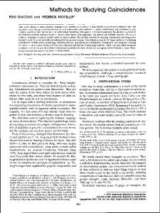
Fig. 2. Left side: Flow profiles for the DPD-method for various slip lengths in the Poisson-Boltzmann regime. The hydrodynamic boundary positions for the DPD-method are at | z B | = (3.866 ± 0.265)σ. The straight lines represent the theoretical prediction of Eqn.(20). Right side: Flow profile for the DPD-(circles) and the LB-method (triangles) with no-slip boundary conditions and Ex = 1.0 /eσ. The straight line is the theoretical prediction of Eqn. (20) with | z B | = 4.0σ and δB = 0.0σ. From Ref. (Smiatek et al. (2009)). Here, we will illustrate the fully explicit approach at the example of two applications in microchannels. The first one is a comparative study of counterion-induced EOF in symmetric planar slit channels using fully explicit DPD and LB simulations (Smiatek et al. (2009)). The theoretical prediction for the EOF profiles in this case is given by Eq. (20). We have studied such flows by two complementary approaches, DPD and LB, and devised schemes how the model parameters could exactly be mapped onto each other. Fig. 2 demonstrates that the results of DPD and LB simulations are in excellent agreement with each other and with theory. The left graph illustrates remarkable flow enhancement due to slippage already in the presence of small surface slip. The examples shown in Fig. (2) refer to situations where the Poisson-Boltzmann theory is applicable, i.e., the microions are monovalent and the charges on the channel surfaces are moderate. With fully explicit simulations, one can also study regimes

116


20

where the mean-field assumption breaks down. In that case, explicit simulations show that the relation between flow and electrostatic potential, Eq. (19), remains valid even though the ion distribution can no longer be calculated analytically (Smiatek et al. (2009)). The electrophoretic response of polyelectrolytes in symmetric slit channels is considered in our second example. As discussed in Section 2.2.3, it results from the combination of bare electrophoresis and background EOF. From Eqs. (21), (23) and (25), one can derive the relation μt μe = 1+ 0 . μEOF μEOF (1 + δB κs )

(46)

This relation is verified in Fig. 3 (left). We have studied the electrophoresis of a charged polyelectrolyte in several electrolytes with different salt concentrations, confined by charged planar walls with different slip lengths. The behavior of the electrophoretic mobility is in very good agreement with the theoretical prediction. Most notably, the EOF flow may reverse the sign of the electrophoretic mobility, such that the polyelectrolyte migrates against the applied field. Following the discussion in Section 2.2.3, we expect the bare mobility of the polyelectrolytes to be independent of chain length in solvents of high ionic strength. Fig. 3 (right) demonstrates that this is indeed the case. 0.5

3 2

0.4

-1000 -1500 0

1

δ = 14.98 σ

]

-500

1/2

0

4

μe [eσ/(mε)

5 xcm [σ]

μt/|μEOF|

6

200

400

600

800

0.2

δ = 0.0 σ

0.1

1/2

t [σ(m/ε)

B

0.3

]

0

B

0

-1 -5

0

5

10

15

20 δBκ

25

30

35

40

0

5

10

15

20 Nm

25

30

35

40

Fig. 3. Left side: Ratio μ t /| μ EOF | plotted against δB κs for chains of length Nm = 20 and several slip lengths and salt concentrations. The black line is the theoretical prediction of Eqn. (46). The ratio μ e /μ0EOF has been fitted to −3.778 ± 0.128. Negative values of μ t /| μ EOF | indicate negative total mobilities of the polyelectrolyte. Inset: Total displacement of the polyelectrolyte’s center of mass for different boundary conditions and a salt concentration of ρs = 0.05625σ−3 . in units of the ion diameter σ. The total mobility becomes negative for | μ e | | μ EOF |. The lines correspond from top to bottom to the slip lengths δB ≈ (0.00, 1.292, 1.765, 2.626, 5.664, 14.98)σ. Thus larger slip lengths indirectly enhance the total mobility of the polyelectrolyte. Right side: Bare electrophoretic mobility for different monomer lengths Nm in confined geometry in the presence of salt for two slip lengths. Finally in this section, we mention a special boundary effect which has not been discussed so far and is often neglected in electrokinetic simulations: The dielectric contrast between water and typical microchannel materials is very high. Therefore, the surfaces are polarized and charges are induced at the boundaries. Tyagi et al. have recently developed a general method that allows one to account for this effect (Tyagi et al. (2007; 2010)). First preliminary studies


117 21

seem to indicatethat it does not influence the transport properties very much on length scales larger than the Debye length. 3.2.2 Fully implicit models

In fully implicit approaches, both solvent and microion degrees of freedom are disregarded and their effect on the particles is incorporated in effective interactions and an effective mobility matrix (see Eq. (42)). This implies an adiabatic approximation: Both the hydrodynamic flows and the local microion distributions are assumed to adjust instantaneously to the macroion configuration. Whereas this approximation can be justified in the case of flows at low Reynolds numbers (as discussed in Section 3.1.4), it is somewhat questionable in the case of the ions. We have discussed important phenomena in Section 2.2 which cannot be captured within such an approach, e.g., the relaxation effect in electrophoresis. Relaxation processes in the ionic double layer of charged colloids have characteristic time scales ranging from microseconds (Maxwell-Wagner relaxation, ionic migration sets in) to 10 milliseconds (the thickness of the Debye layer adjusts), which is close to the characteristic time scales of many mesoscale simulations. Thus fully implicit methods are hardly suited for studying dynamical processes with a time evolution. They can however be used to study quasi-stationary situtaions such as electrophoresis or pressure-driven transport at a semi-quantitative level. A second drawback of implicit schemes is that they usually rely on the Debye-Hückel approximation, which has a limited range of validity as discussed in Section 2.2.1. Nevertheless, it can often be applied successfully even in the nonlinear regime as long as one accounts for nonlinear effects by appropriate charge renormalization or renormalization of the local Debye Hückel screening length (see 2.2.1). Fully implicit simulations are stochastic simulations with the structure of BD simulations (Eq. (42)). Setting up BD schemes for nanoparticles in external electric fields is slightly subtle due to the fact that one has two mobility matrices: One (DC ) which describes the hydrodynamic interactions in response to conservative forces and is related to the unscreened Greens function Eq. (8) or (45) in free solution, and one (D E ) which describes the hydrodynamic interactions in response to external electric fields, and can be related to the screened Greens function (29) in free solution if the external fields vary slowly compared to the Debye Hückel screening length. A clean way of dealing with this situation is to treat both types of responses on separate footings: In a constant or slowly varying electric field E and external flow field u (r ), the equation of motion of a system of particles i with charges q i (the equivalent of Eq. (42) ) is then given by (Kekre et al. (2010)) C C E r˙ iα = u α (ri ) + ∑ ∑ Diα,jβ Fjβ + ∑ ∑ ξ iα,jβ θ jβ + ∑ ∑ Diα,jβ q j Eβ , j

β

j

β

j

β

where DC and D E are given by ( 0)

C = δij δαβ μ i Diα,jβ C Diα,jβ

+ (1 − δij ) Tαβ (ri −r j )

= δij δαβ μ i + (1 − δij ) Gαβ (ri −r j ) el

(47)

118


22

( 0)

and the matrix ξ meets the requirement ξξ T = DC . Here μ i is the bare frictional mobility of the particle i, μeli its electrophoretic mobility, and T, G are the screened and unscreened hydrodynamic Greens functions, which can be approximated by the Rotne-Prager tensor (45) and the screened Greens function (29) (or the corresponding Rotne-Prager version (Fischer et al. (2008))) in free solution. It is important to note that FjC subsumes all effective conservative interactions between ions, including those of electrostatic origin. One can show rigorously that a procedure where (microion) degrees of freedom are integrated out adiabatically only renormalizes the conservative potentials of the remaining macroions and not their mobility coefficients. Thus, the Coulomb potentials are replaced by screened Yukawa potentials, but the hydrodynamic interactions remain long-range. The situation is different in electrophoresis since this is an inherently nonequilibrium process. Solving Eq. (47) for many-particle systems is expensive due to the long-range hydrodynamic interactions and the noise issue discussed in Section 3.1.4. If the dominating forces in a system are due to external electric fields, it may become acceptable to neglect the long-range hydrodynamic contributions. In nanochannels, this approximation can further be justified by the fact that hydrodynamic interactions are screened in confinement (see Section 2.1.2). For these reasons, simulation approaches have been popular already early on where both hydrodynamics and electrostatics were neglected entirely. The motion of macroions in an external electric field E (r ) and flow field u(r ) is then described by simple local Langevin dynamics, where the force Fi on a particle i at position ri is given by the sum

Fi = F C + FiD + FiR i

(48)

of conservative contributions FiC = q i E (ri ) + Fi,Cint , the dissipative drag force FiD = − ζ (vi − u(ri )) and a Gaussian distributed random force FIR which satisfies the fluctuation dissipation relation F R (t) F R (t ) = 2 ζ k B T δij δαβ δ(t − t ). The internal contributions F C iα

jβ

i,int

subsume the screened electrostatic interactions between particles as well as other forces with non-electrostatic origin. The situation is particularly simple if the external flow u(r ) has been generated by EOF and the channel has the similitude property (Section 2.2.2), i.e., u(r ) = μEOFE(r ). In that case, the total force on the particle i is given by

Fi = F C + (q i + μEOF ζ )E (ri ) − ζvi + FiR . i,int

(49)

Thus the EOF flow u (r ) simply has the effect of renormalizing the charge q i (Streek et al. (2005)). Simple local BD approaches such as Eq. (49) have been used quite successfully to study electrophoresis in complex geometries, and they can yield good qualitative and even semiquantitative agreement with experiments (Streek et al. (2004); Viovy (2000)). As an example, Fig. 4 shows results from such a BD simulation of DNA electrophoresis in a structured microchannel. Both in experiments and simulations, one observes a two-state behavior where the DNA switches between a ”slow” and ”fast” migration mode. This is reflected by an inhomogeneous average monomer distribution in the channel (Streek et al. (2005)).


119 23

a) a)

b) a)

b)c)

c)d)

Fig. 4. Top panel (a): Monomer density histograms obtained from local BD simulation of electrophoresis of charged chains with different lengths N = 50, 100, 120, 140 (top, left to right) and N = 170, 200, 250 and 320 (bottom) at. Bottom panel: Monomer density histograms obtained from experiment at applied voltages (b) E = 43V/cm, (c) E = 86V/cm, and (d) E = 130V/cm for λ-DNA in 5μm constrictions. The fluorescence intensity decreases because the illumination time was kept constant. Note the depletion zone in the center of the channel. From (Streek et al. (2005)) Despite these successes, the complete neglect of hydrodynamic interactions sometimes simplifies the situation too much even in simulations of electrophoretic transport. In these cases, one may still choose to work with the screened hydrodynamic Greens function G for reasons of efficiency and neglect the unscreened contributions. Löwen et al have demonstrated that such a scheme can be used successfully to describe the effect of hydrodynamic interactions in systems of oppositely charged colloids subject to an external field. Even the screened hydrodynamic interactions have a noticeable effect on structure formation and ”laning” in such systems (Rex & Löwen (2008)). 3.2.3 Mixed schemes

Mixed schemes for electrohydrodynamic simulations treat either the solvent or the microions at an implicit level. In the first approach, both microions and macroions are represented by explicit particles which interact with each other by means of the full Rotne-Prager tensor, Eq. (45) (Fischer et al. (2008); Kim & Netz (2006)). These methods are motivated by the fact mentioned earlier that hydrodynamic flows adjust very rapidly, whereas ion rearrangement processes can be slow on mesoscopic time scales. Unfortunately, they suffer from the bad scaling properties of BD simulations and have therefore not been used to study very large systems. In the second type of approach, the solvent is modeled as an explicit fluid, but microions are no longer represented by individual particles. Many kinetic processes in electrolyte solutions

120


24

do not depend on ion correlations and can thus be described satisfactorily at the mean-field level. To access larger length scales in simulations, one may therefore resort to methods that treat the ions at the level of the Nernst-Planck equation (12). So far, efforts to develop such methods have mainly focused on LB approaches (Capuani et al. (2004); Horbach & Frenkel (2001); Pagonabarraga et al. (2005); Warren (1997)). A number of authors have proposed simplified schemes that capture basic electrokinetic phenomena at a heuristic level in explicit fluid simulations. For example, one simple way to deal with EOF is to impose a velocity boundary condition (Eq. (23)) at the walls of a microfluidic channel (Duong Hong et al. (2008)). Similarly, the electrohydrodynamic screening effect in electrophoresis can be mimicked in a LB simulation by adding a slip D term to the Stokes drag on the particle in the LB flow. The dissipative contribution F = − u (R, t) to Eq. (40) is then replaced by a modified drag force (Hickey et al. (2010)) −ζ V − u(R, t) − μ0E F D = −ζ V

(50)

Unfortunately, this elegant idea cannot easily be transferred to DPD and MPCD simulations. Duong-Hong et al. have proposed an alternative approach where charges are assigned to DPD or MPCD particles that are within a certain distance (the Debye length) of the macroions or charged walls. These particles are then dragged along by the electric field, which can be used to mimick electrophoretic retardation, electrohydrodynamic screening effects, and EOF generation on channel surfaces in a unified manner (Duong Hong et al. (2008b)).

4. Summary and outlook With the advent of faster computers and improved simulation methods for electrostatics and hydrodynamics, electrohydrodynamic simulations become an increasingly attractive tool for studying and predicting electrokinetic phenomena in microgeometries. In this chapter we have introduced the main concepts behind coarse-grained mesoscale simulations of microand nanofluidic flow and transport. We have focused on boundary effects and mean-field phenomena, e.g., phenomena that can be rationalized within the Poisson-Boltzmann theory. Several important phenomena such as counterion condensation, overcharging, shape transformations of the polyelectrolytes, confinement effects, to name a few, have not been discussed in this work. Also, important problems of current interest such as electrophoresis with obstacle collisions or polymer nanopore translocations, have not been mentioned. For further reading, we refer the interested reader to the reviews (Boroudjerdi et al. (2005); Graham (2011); Pagonabarraga et al. (2010); Slater et al. (2009); Viovy (2000)). We have shown that mesoscopic simulation methods are powerful tools to explore fluid behavior on the micro- and nanoscale. Such simulations not only help to understand and optimize transport processes in micro- and nanofluidic channels, they can also be used to study basic mechanisms for many physical processes of life, since such processes often take place in confinement (e.g., cells) and in aqueous solutions with high ion concentrations. We expect that the mesoscale techniques introduced in this chapter, combined with microscopic and macroscopic approaches, will open new routes towards a better understanding of transport phenomena on the micro- and nanoscale.


121 25

5. Acknowledgments We have benefitted from discussions with Mike P. Allen, Burkhard Dünweg, Ralf Eichhorn, Kai Grass, Christian Holm, Sebastian Meinhardt, Ulf D. Schiller, Marcello Sega, Martin Streek, and Tatiana Theis. The fully explicit simulations presented here have been carried out using the software package ESPResSo (http://www.icp.uni-stuttgart.de/∼icp/ESPResSo) (Arnold et al. (2006)). We thank the Volkswagen Stiftung and the Deutsche Forschungsgemeinschaft for funding and the HLR Stuttgart, NIC Jülich and Arminius PC2 -cluster in Paderborn for computing times.

6. References Ahlrichs, P. & Dünweg, B. (1999). Simulation of a single polymer chain in solution by combining Lattice Boltzmann and molecular dynamics. Journal of Chemical Physics Vol. 111, 8225. Ahmed, N.K. & Hecht, M. (2009). A boundary condition with adjustable slip length for Lattice Boltzmann simulations. Journal of Statistical Physics Vol. 2009, P09017. Alexander, S.; Chaikin, P.M.; Grant, P.; Morales, G.H. ; Pincus, P. & Hone, D. (1984). Charge renormalization, osmotic pressure, and bulk modulus of colloidal crystals: Theory. Journal of Chemical Physics, Vol. 80, 5776. Arnold, A.; Mann, B.A.; Limbach, H.-J. & Holm, C. (2006). ESPResSo - An Extensible Simulation Package for Research on Soft Matter Systems. Computer Physics Communications, Vol. 174, 704. Banchio, A.J. & Brady, J.F. (2003). Accelerated Stokesian Dynamics: Brownian motion. Journal of Chemical Physics Vol. 118, 10323. Barrat, J.-L. & Joanny, J. F. (1996). Theory of polyelectrolyte solutions. Advances in Chemical Physics Vol. 94, 1. Bocquet, L. & Barrat, J.-L. (1994). Hydrodynamic boundary conditions, correlation functions, and Kubo relations for confined fluids. Physical Review E Vol. 49, 3079. Benzi, R.; Succi, S. & Vergassola, M. (1992). The Lattice Boltzmann equation: Theory and applications. Physics Reports Vol. 22, 145. Bhatnagar, P. L., Gross, E. P. & Krook, M. (1954). A model for collision processes in gases. 1. Small amplitude proceesses in charged and neutral one-component systems. Physical Review Vol. 54, 511. Boroudjerdi, H.; Kim, Y. -W.; Najim A.; Netz, R. R.; Schlagberger, X. & Serr, A. (2005). Statics and dynamics of strongly charged soft matter. Physics Reports Vol. 416, 129. Bouzigues, C.I.; Tabeling, P. & Bocquet, L. (2008). Nanofluidics in the Debye Layer at Hydrophilic and Hydrophobic Surfaces. Physical Review Letters, Vol. 101, Article-No. 114503. Capuani, F.; Pagonabarraga, I. & Frenkel, D. (2004). Discrete solution of the electrokinetic equations. Journal of Chemical Physics Vol. 121, 973. Chen, S. & Doolen, G. D. (1998). Lattice-Boltzmann method for fluid flows. Annual Review of Fluid Mechanics Vol. 30, 329. Cui, B.; Diamant, H. & Lin, B. (2002). Screened Hydrodynamic Interactions in a Narrow Channel. Physical Review Letters Vol. 89, Article-No. 188302.

122

26


Cummings, E.B.; Griffiths, S. K.; Nilson, R. H.; & Paul, P. H. (2000). Conditions for similitude between the fluid flow and electric field in electroosmotic flow. Analytical Chemistry Vol. 72, 2526. Diamant, H.; Cui, B.; Lin, B. & Rice, S.A. (2005). Hydrodynamic interactions in quasi-two-dimensional suspensions. Journal of Physics: Condensed Matter, Vol. 17, S2787. Dhont, J.K.G. (1996). An Introduction to Dynamics of Colloids. Elsevier, Amsterdam. Doi, M. & Edwards, S. F. (1986). The Theory of Polymer Dynamics. Oxford Science Publications, Oxford. Dufresne, E.R.; Squires, T.M.; Brenner, M.P. & Grier, D.G. (2000). Hydrodynamic coupling of two Brownian spheres to a planar surface. Physical Review Letters, Vol. 85, 3317. Duong-Hong D.; Wang, J.-S.; Liu, G.R.; Chen, Y.Z.; Han, J. & Hadjiconstantinou, N.G. (2008). Dissipative simulations of electroosmotic flow in nanofluidic devices. Microfluidics and Nanofluidics Vol. 4, 219. Duong-Hong, D.; Han, J.; Wang, J.-S.; Hadjiconstantinou, N.G.; Chen, Y.Z. & Liu, G.-R. (2008). Realistic simulations of combined DNA electrophoretic flow and EOF in nanofluidic devices. Electrophoresis Vol. 29, 4880. Dünweg, B., Schiller, U. & Ladd, A.J.C (2007). Statistical mechanics of the fluctuating Lattice Boltzmann equation. Physical Review E Vol. 76, 036704. Dünweg, B. & Ladd, A.J.C (2009). Lattice Boltzmann simulations of soft matter systems. Advances in Polymer Science Vol. 221, 89. Ermak, D. L. & McCammon, J. A. (1978). Brownian dynamics with hydrodynamic interactions. Journal of Chemical Physics Vol. 69, 1352. Español, P. & Warren, P. B. (1995). Statistical mechanics of dissipative particle dynamics. Europhysics Letters Vol. 30, 191. Fischer, S.; Naji, A. & Netz, R.R. (2008). Salt-induced counterion-mobility anomaly in polyelectrolye electrophoresis. Physical Review Letters, Vol. 101, 176103. Fixman, M. (1986). Construction of Langevin forces in the simulation of hydrodynamic interactions. Macromolecules Vol. 19, 1204. Frenkel, D. & Smit, B. (2001). Understanding molecular simulation. Academic Press, Orlando. Frisch, U.; Hasslacher, B. & Pomeau, Y. (1986). Lattice Automata for the Navier-Stokes Equation. Physical Review Letters Vol. 56, 1505. Geyer, T. & Winter, U. (2009). An O( N 2 ) approximation for hydrodynamic interactions in Brownian dynamics simulations. Journal of Chemical Physics Vol. 130, 114905. Gompper, G.; Ihle, T.; Kroll, K. & Winkler. R. G. (2009). Multi-particle collision dynamics: A particle-based mesoscale simulation approach to the hydrodynamics of complex fluids. Advances in Polymer Science Vol. 221, 1. Graham, M. D. (2011). Fluid dynamics of dissolved polymer molecules in confined geometry. Annual Review of Fluid Mechanics Vol. 43, 273. Grass, K.; Böhme, U.; Scheler, U.; Cottet, H. & Holm, C. (2008). Importance of hydrodynamic shielding for the dynamic behavior of short polyelectrolyte chains. Physical Review Letters Vol. 100, Article-No. 096104. Frank, S. & Winkler, R.G. (2008). Polyelectrolyte electrophoresis: Field effects and hydrodynamic interactions. Europhysics Letters Vol. 83, 38004. Groot, R. D. & Warren, P. B. (1997). Dissipative particle dynamics: Bridging the gap between atomistic and mesoscopic simulations. Journal of Chemical Physics Vol. 107, 4423.


123 27

Happel, J.; Brenner, H. (1983). Low Reynolds Number Hydrodynamics. Martinus Nijhoff. Dordrecht. Hecht, M.; Harting, J. (2010). Implementation of on-site velocity boundary condition for D3Q19. Journal of Statistical Mechanics Vol. 2010, P01018. Hickey, O.A.; Holm, C.; Harden, J.L. & Slater, G.W. (2010). Implicit method for simulating electrohydrodynamics of polyelectrolytes. Physical Review Letters Vol. 105, 148301. Hoogerbrugge, P. J. & Koelman, J. M. V. A. (1992). Simulating microscopic hydrodynamic phenomena with dissipative particle dynamics. Europhysics Letters Vol. 19, 155. Horbach, J. & Frenkel, D. (2001). Lattice-Boltzmann method for the simulation of transport phenomena in charged colloids. Physical Review E Vol. 64, Article-No. 051607. Hunter, R. J. (1991). Foundations of Colloid Science. Clarendon Press, Oxford. Ihle, T. & Kroll, D.M. (2003). Stochastic rotation dynamics. I. Formalism, Galilean invariance, and Green-Kubo relations. Physical Review E Vol. 67, 066705. Israelachvili, J. (1991). Intermolecular and surface forces. Academic Press. London. Joly, L.; Ybert, C.; Trizac, E. & Bocquet, L. (2004). Hydrodynamics within the electric double layer on slipping surfaces. Physical Review Letters, Vol. 93, Article-No. 257805. Joly, L.; Ybert, C.; & Bocquet, L. (2006). Probing the nanohydrodynamics at liquid-solid interfaces using thermal motion. Physical Review Letters, Vol. 96, Article-No. 04601. Kekre, R.; Butler, J.E.; Ladd, A.J.C. (2010). A comparison of lattice-Boltzmann and Brownian dynamics simulations of a polymer migration in confined flows. Physical Review E, Vol. 82, Article-No. 011802. Kekre, R.; Butler, J.E.; Ladd, A.J.C. (2010). Role of hydrodynamic interactions in the migration of polyelectrolytes driven by a pressure gradient and an electric field. Physical Review E, Vol. 82, Article-No. 050803(R). Kennard, E. H. (1938). Kinetic theory of gases. McGraw-Hill, New York. Kim, K.; Nakayam, Y. & Yamamoto R. (2006). Direct Numerical Simulations of electrophoresis of Charged Colloids. Physical Review Letters, Vol. 79, 031401. Kim, Y.W. & Netz, R.R. (2006). Electroosmosis at inhomogeneous charged surfaces: Hydrodynamic versus electric friction. Journal of Chemical Physics, Vol. 124, 114709. Kjellander, R. & Mitchell D.J. (1994). Dressed-ion theory for electrolyte solutions: A Debye-Hückel like reformulation of the exact theory for the primitive model. Journal of Chemical Physics Vol. 101, 603. Koelman, J. M. V. A. & Hoogerbrugge P. J. (1993). Dynamic simulation of hard sphere suspensions under steady shear. Europhys. Lett. Vol. 21, 363. Kuang, C. & Wang, G. (2010). A novel far-field nanoscopic velocimetry for nanofluidics. Lab Chip Vol. 10, 240. Kunert, C. & Harting, J.D.R. (2008). Simulation of fluid flow in hydrophobic rough microchannels. International Journal of Computational Fluid Dynamics Vol. 22, 475. Ladd, A.J.C. (1994). Numerical simulations of particulate suspensions via a discretized Boltzmann equation Part I: Theoretical foundations. Journal of Fluid Mechanics Vol. 271, 285. Ladd, A.J.C. (1994). Numerical simulations of particulate suspensions via a discretized Boltzmann equation Part II: Numerical Results. Journal of Fluid Mechanics Vol. 271, 311. Landau, L. D.; Lifshitz, E. M. (1987). Fluid Mechanics. Volume 6 (Course of Theoretical Physics). Butterworth-Heinemann. Oxford.

124

28


Lamura, A.; Gompper, G.; Ihle, T.; Kroll, D. (2001). Multi-particle collision dynamics: Flow around a circular and a square cylinder. Europhysics Letters Vol. 56, 319. Liron, N. & Mochon, S. (1976). Stokes flow for a stokeslet between two parallel flat plates. Journal of Engineering Mathematics, Vol. 10, 287. Lobaskin, V. & Dünweg, B. (2004). A new model for simulating colloidal dynamics. New Journal of Physics Vol. 6, 54. Long, D. & Ajdari, A. (2001). A note on the screening of hydrodynamic interactions, in electrophoresis, and in porous media. European Physical Journal E Vol. 4, 29. Lyklema, J. (1995). Fundamentals of Interface and Colloid Science. Academic Press. New York. Malevanets, A. & Kapral, R. (1999). Mesoscopic model for solvent dynamics. Journal of Chemical Physics Vol. 110, 8605. Malevanets, A. & Kapral, R. (2000). Solute dynamics in mesoscale solvent. Journal of Chemical Physics Vol. 112, 7260. Manning, G. S. (1981). Limiting laws and counterion condensation in polyelectrolyte solutions. 7. Electrophoretic mobility and conductance. Journal of Physical Chemistry Vol. 85, 1506. Marsh, C.; Backx, G. & Ernst, M.H. (1997). Static and dynamic properties of dissipative particle dynamics. Physical Review E Vol. 56, 1976. McBride, A.; Kohonen, M. & Attard, P. (1998). The screening length of charge-asymmetric electrolytes: A hypernetted chain calculation. Journal of Chemical Physics Vol. 109, 2423. McNamara, G. R. & Zanetti, G. (1988). Use of the Boltzmann equation to simulate Lattice-Gas Automata. Physical Review Letters Vol. 61, 2332. Mitchell, D.J. & Ninham, B.W. (1978). Range of the screened Coulomb interaction in electrolytes and double layer problems. Chemical Physics Letters Vol. 53, 397. Neto, C.; Evans, D. R.; Bonaccurso, E.; Butt, H.-J. & Craig V. S. J. (2005). Boundary slip in Newtonian liquids: A review of experimental studies. Report on Progress in Physics Vol. 68, 2859. Noguchi, H, ; Kikuchi, R. & Gompper, G. (2007). Particle-based mesoscale hydrodynamic techniques. Europhysics Letters Vol. 78, 10005. Onsager, L. (1926). Zur Theorie der Elektrolyte 1. Physikalische Zeitschrift Vol. 27, 388. Onsager, L. (1927). Zur Theorie der Elektrolyte 2. Physikalische Zeitschrift Vol. 28, 277. Onsager, L. & Fuoss, R. M. (1932). Irreversible processes in electrolytes. Diffusion, conductance, and viscous flow in arbitrary mixtures of strong electrolytes. Journal of Physical Chemistry Vol. 36, 2689. Pagonabarraga, I.; Capuani, F. & Frenkel, D. (2005). Mesoscopic lattice modeling of electrokinetic phenomena. Computer Physics Communications Vol. 169, 192. Pagonabarraga, I.; Rotenberg, B. & Frenkel, D. (2010). Recent advances in the modelling and simulation of electrokinetic effects: Bridging the gap between atomistic and macroscopic descriptions. Physical Chemistry Chemical Physics Vol. 12, 9566-9580. Pit, R.; Hervet, H. & Leger, L. (2000). Direct experimental evidence of slip in hexadecane:solid interfaces. Physical Review Letters Vol. 85, 980. Pivkin, I.V., Caswell, B. & Karniadakis, G.E. (2010). Dissipative particle dynamics. Reviews in Computational Chemistry, Vol. 27 (ed. K.B. Lipkowitz), John Wiley & Sons, Ind., Hoboken, NJ, USA.


125 29

Revenga, M.; Zuniga, I.; Español, P. & Pagonabarraga, I. (1998). Boundary models in dissipative particle dynamics. International Journal of Modern Physics C Vol. 9, 1319. Revenga, M.; Zuniga, I. & Español P. (1999). Boundary Conditions in Dissipative Particle Dynamics. Computer Physics Communications Vol. 121-122, 309. Rex, M. & Löwen, H. (2008). Influence of hydrodynamic interactions on lane formation in oppositely charged driven colloids. European Physical Journal E Vol. 26, 143 Rotne, J. & Prager, S. (1969). Variational treatment of hydrodynamic interactions in polymers. Journal of Chemical Physics Vol. 50, 4831. Slater, G. W.; Holm, C.; Chubynsky, M. V.; de Haan, H. W.; Dube, A.; Grass, K.; Hickey, O. A.; Kingsburry, C.; Sean, D.; Shendruk, T. N. & Nhan, L. X. (2009). Modeling the separation of macromolecules: A review of current computer simulation methods. Electrophoresis Vol. 30, 792. Smiatek, J.; Allen, M. P. & Schmid, F. (2008). Tunable slip boundaries for coarse-grained simulations of fluid flow. European Physical Journal E Vol. 26, 115. Smiatek, J. (2009). Mesoscopic simulations of electrohydrodynamic phenomena. PhD thesis. Bielefeld Unversity, Bielefeld. Smiatek, J.; Sega, M.; Schiller, U. D.; Holm, C. & Schmid, F. (2009). Mesoscopic simulations of the counterion-induced electro-osmotic flow: A comparative study. Journal of Chemical Physics Vol. 130, 244702. Smiatek, J.; Schmid, F. (2010). Polyelectrolyte electrophoresis in nanochannels: A dissipative particle dynamics simulation. Journal of Physical Chemistry B Vol. 114, 6266. Smiatek, J. & Schmid, F. (2011). Mesoscopic simulations of electroosmotic flow and electrophoresis in nanochannels. Computer Physics Communications Vol. 182, 1941. Soddemann, T.; Dünweg, B. & Kremer, K. (2003). Dissipative particle dynamics: A useful thermostat for equilibrium and nonequilibrium molecular dynamics simulations. Physical Review E Vol. 68, 046702. Sparreboom, W.; van den Berg, A. & Eijkel, J.T.C. (2010). Transport in nanofluidic systems: A review of theory and applications. New Journal of Physics Vol. 12, 015004. Streek, M.; Schmid, F.;, Duong, T. T. & Ros, A. (2004). Mechanisms of DNA separation in entropic trap arrays: A Brownian dynamics simulation. Journal of Biotechnology Vol. 112, 79. Streek, M.; Schmid, F.;, Duong, T. T.; Anselmetti, D. & Ros, A. (2005a). Two-state migration of DNA in a structured microchannel. Physical Review E Vol. 71, 011905. Succi, S. (2001). The Lattice Boltzmann equation for fluid dynamics and beyond, Oxford University Press, USA. Succi, S. (2002). Mesoscopic modeling of slip motion at fluid-solid interfaces with heterogeneous catalysis. Physical Review Letters Vol. 89, 064502. Sutmann, G. (2009). ScaFaCoS – when long range goes parallel. Innovative Supercomputing in Deutschland Vol. 7, No. 1. Tlusty, T. (2006). Screening by symmetry of long-range hydrodynamic interactions of polymers confined in sheets. Macromolecules, Vol. 39, 3927. Tretheway, D.& Meinhart, C. (2002). Apparent fluid slip at hydrophobic microchannel walls. Physics of Fluids Vol. 14, 9. Trizac, E.; Bocquet, L. & Aubouy, M. (2002). Simple approach for charge renormalization in highly charged macroions. Physical Review Letters, Vol. 89, Article-No. 248301.

126

30


Tyagi, S.; Arnold, A. & Holm, C. (2007). ICMMM2D: An accurate method to include planar dielectric interfaces via image charge summation. Journal of Chemical Physics Vol. 127, 154723. Tyagi, S.; Süzen, M.; Sega, M.; Barbosa, M.; Kantorovich, S. & Holm, C. (2010). An iterative, fast, linear-scaling method for computing induced charges on arbitrary dielectric boundaries. Journal of Chemical Physics Vol. 132, 154112. Viovy, J.-L. (2000). Electrophoresis of DNA and other polyelectrolytes: Physical mechanisms. Review of Modern Physics, Vol. 72, 813. Warren, P.B. (1997). Electroviscous transport problems via Lattice Boltzmann. International Journal of Modern Physics C Vol. 8, 889. Whitmer, J, & Luijten, E. (2010). Fluid-solid boundary conditions for multiparticle collision dynamics. J. Phys.: Cond. Matter Vol. 22, 104106. Wright, M. R. (2007). An introduction to aqueous electrolyte solutions, John Wiley & Sons, Chichester. Yamakawa, H. (1970). Transport properties of polymer chains in dilute solution: Hydrodynamic interaction. Journal of Chemical Physics Vol. 53, 436. Yeomans, J. M. (2006). Mesoscopic simulations: Lattice Boltzmann and particle algorithms. Physica A Vol. 369, 159. Zou, Q. & He, X. (1997). On pressure and velocity boundary conditions for the Lattice Boltzmann BGK model. Physics of Fluids Vol. 9, 1591.

Mesoscopic Simulation Methods for Studying Flow

Mesoscopic Simulation Methods for Studying Flow

Suggest Documents

Methods for Numerical Flow Simulation

LABORATORY SIMULATION METHODS FOR STUDYING ... - People

Methods for Studying Coincidences

Methods for Studying Leadership - Corwin

Methods for Studying Leadership - HEC

Introduction to Direct Simulation Methods for Rarefied Flow - UQ eSpace

Multiscale methods for two and three-phase flow simulation in ...

FLOW CHAMBER FOR STUDYING CELL ATTACHMENT TO ...

A Simulation Approach for Studying Behavior and

REGIONAL MICROSCOPIC SIMULATION MODEL FOR STUDYING ...

C3Conflict a Simulation Environment for Studying

Some Methods for Studying Cultural Cognitive ...

methods for studying morphological integration and modularity

methods for studying morphological integration and modularity

methods for studying morphological integration and modularity

Mathematical and Computational Methods for Studying Energy

Culture-independent methods for studying environmental ...

Chemometric Methods for Studying the Relationships ...

Algebraic Methods for Studying Interactions Between Epidemiological

Methods for studying information provision ...

Three computational methods for studying permeation ... - CiteSeerX

research methods and methodologies for studying ... - CiteSeerX

Research Methods for Studying ABE/ESOL Populations

NEW MEASUREMENT METHODS FOR STUDYING ...